Annealed transition density of simple random walk
on a high-dimensional loop-erased random walk
Abstract
We derive sub-Gaussian bounds for the annealed transition density of the simple random walk on a high-dimensional loop-erased random walk. The walk dimension that appears in these is the exponent governing the space-time scaling of the process with respect to the extrinsic Euclidean distance, which contrasts with the exponent given by the intrinsic graph distance that appears in the corresponding quenched bounds. We prove our main result using novel pointwise Gaussian estimates on the distribution of the high-dimensional loop-erased random walk.
AMS 2020 MSC: 60K37 (primary), 05C81, 60J35, 60K35, 82B41.
Keywords and phrases: heat kernel estimates, loop-erased random walk, random walk in random environment.
1 Introduction
The main result of this article provides annealed heat kernel estimates for the random walk on the trace of a loop-erased random walk in high dimensions. Whilst this is something of a toy model, the statement reveals an interesting difference between the quenched (typical) heat kernel estimates, which are of Gaussian form with respect to the intrinsic graph metric, and the annealed (averaged) heat kernel estimates, which are of sub-Gaussian form with respect to the extrinsic Euclidean metric. (We will present more detailed background concerning this terminology below.) Establishing such a discrepancy rigourously was motivated by a conjecture made in [6, Remark 1.5] for the two-dimensional uniform spanning tree, and naturally leads one to consider to what extent the behaviour is typical for random walks on random graphs embedded into an underlying space.
Before describing further our heat kernel estimates, we would like to present the key input into their proof, which is a time-averaged Gaussian bound on the distribution of the loop-erased random walk. In particular, throughout the course of the article, we let be the loop-erasure of the discrete-time simple random walk on , where , started from the origin. (See Section 2 for a precise definition of this process, which was originally introduced by Lawler in [19].) In the dimensions we are considering, it is known that the loop-erased random walk (LERW) behaves similarly to the original simple random walk (SRW), in that both have a Brownian motion scaling limit; for the SRW, this follows from the classic invariance principle of Donsker [13], whereas for the LERW, it was proved in [19]. Taking into account the diffusive scaling, such results readily imply convergence of the distributions of and as . For our heat kernel estimates, we will require understanding of the distribution of LERW on a finer, pointwise scale. Now, one can check that SRW satisfies pointwise Gaussian bounds of the form
| (1) |
where is a constant and we write for the -norm of , see [3, Theorem 6.28], for example. (The averaging over two time steps is necessary for parity reasons.) Of course, one can not expect the same bounds for a LERW. Indeed, the ‘on-diagonal’ part of the distribution is equal to zero for . What we are able to establish is the following, which demonstrates that if one averages over longer time intervals, then one still sees Gaussian behaviour.
Theorem 1.1.
The loop-erased random walk on , , started from the origin satisfies the following bounds: for all , ,
and for all , ,
where are constants.
Remark 1.2.
Another random path known to scale to Brownian motion in dimensions is the self-avoiding walk (SAW) [14, 15]. A local central limit theorem for a ‘spread out’ version of the SAW was established in [23]. For a precise statement, one should refer to [23, Theorem 1.3], but roughly it was shown that if is the number of -step self-avoiding walk paths from 0 to and , then, for appropriate constants and , as ,
where is an -ball and is a divergent sequence satisfying . (We note that the term in [23] can be replaced by by applying [24, Theorem 1.1].) In particular, the left-hand side here can be thought of as the probability a self-avoiding walk of length is close to , with the ball over which the spatial averaging is conducted being microscopic compared with the diffusive scaling of the functional scaling limit. For the LERW of this article, one might ask if it was similarly possible to reduce the intervals over which time averaging is conducted in Theorem 1.1 to ones of the form where . And, for both the LERW and the SAW, one could ask for what ranges of the variables a pointwise space-time bound as at (1) holds. See [2] for a result in this direction concerning the weakly self-avoiding walk.
We now introduce our model of random walk in a random environment. To this end, given a realisation of , we define a graph to have vertex set
and edge set
We then let be the continuous-time random walk on that has unit mean exponential holding times at each site and jumps from its current location to a neighbour with equal probability being placed on each of the possibilities. Moreover, we will always suppose that . Clearly, since equipped with its shortest-path graph metric is isometric to , it is straightforward to deduce that, for each realisation of ,
| (2) |
in distribution, where is a one-dimensional Brownian motion started from 0, and we can also give one-dimensional Gaussian bounds for the transition probabilities of on (see Lemma 4.1 below). In this article, though, we are interested in the annealed situation, when we average out over realisations of . Precisely, we define the annealed law of to be the probability measure on the Skorohod space given by
where is the probability measure on the underlying probability space upon which is built, and is the law of on the particular realisation of (i.e. the quenched law of ). We are able to prove the following. Note that we use the notation and .
Theorem 1.3.
For any , there exist constants such that, for every and ,
and also
Remark 1.4.
Essentially similar arguments would apply if was replaced by the discrete-time simple random walk on . In that case, one would need to assume for the lower bound, since the probability being estimated would be zero for . In the continuous setting, the behaviour of takes on a different form for , as the probability will be determined by certain rare events (cf. the discussion of Poisson bounds in [3, Section 5.1]; see also Lemma 4.1 below).
To put this result into context, it helps to briefly recall what kind of behaviour has been observed for anomalous random walks and diffusions in other settings. In particular, for many random walks or diffusions on fractal-like sets (either deterministic or random), it has been shown that the associated transition density satisfies, within appropriate ranges of the variables, upper and lower bounds of the form
| (3) |
where is some metric on the space in question. (See [3, 18] for overviews of work in this area.) The exponent is typically called the spectral dimension, since it is related to growth rate of the spectrum of the generator of the stochastic process. The exponent , which is usually called the walk dimension (with respect to the metric ), gives the space-time scaling.
Now, in our setting, we can clearly write
and, moreover, using simple facts about the intersection properties of SRW in high dimensions, one can check that (where we use the notation to mean that the left-hand side is bounded above and below by constant multiples of the right-hand side). Hence, Theorem 1.3 gives that satisfies upper and lower bounds of exactly the sub-Gaussian form at (3), with , and being the Euclidean metric. We can understand that results from one-dimensional nature of the graph with respect to its intrinsic metric . Moreover, the exponent gives the space-time scaling of the process with respect to the Euclidean metric. Indeed, it is not difficult to combine (2) and the Brownian motion scaling limit of (from [19]) to check that, up to a deterministic constant factor in the time scaling,
where is a -dimensional Brownian motion, independent of the one-dimensional Brownian motion , with and each started from the origin. (The limit process is a version of the -dimensional iterated Brownian motion studied in [12], for example. Cf. the result in [10] for random walk on the range of a random walk.) We note that the exponent matches the quenched spectral dimension, whereas the is the multiple of the ‘2’ of the quenched bound, which is the walk dimension of with respect to the intrinsic metric , and the ‘2’ that gives the space-time scaling of . We highlight that the annealed bound is not obtained by simply replacing by in the quenched bound, though, as doing that does not result in an expression of the form at (3).
As remarked at the start of the introduction, it was conjectured in [6] that a similar combination of the various exponents will appear in sub-Gaussian annealed heat kernel bounds for the random walk on the two-dimensional uniform spanning tree. In that case, the spectral dimension of the quenched and annealed bounds is known to be , the intrinsic walk dimension is and the exponent governing the embedding is given by the growth exponent of the two-dimensional LERW, i.e. , giving an extrinsic walk dimension of . We are able to check the corresponding result for our simpler model using the simple observation that
| (4) |
and then combining the estimate on the distribution of the LERW from Theorem 1.1 with the deterministic Gaussian bounds on of Lemma 4.1 below. It is clear that a similar argument would apply for other random walks on random paths, including ones with different exponents, whenever one can suitably estimate the term corresponding to . LERW in dimensions , and would represent worthwhile examples to consider here. For more general random graphs, one could give a decomposition that is similar to (4), but to proceed from that point one would need both good quenched heat kernel estimates with respect to some distance in place of the Gaussian bounds on and good estimates on how the distance that appears in the quenched bounds behaves. Pursuing this program would be of interest for various random graphs that do not exhibit homogenisation. Apart from the uniform spanning tree/forest (in two and other dimensions, see [1, 5, 6] for some relevant background on the associated random walk), one might consider the situation for random walk on: the trace of a simple random walk on , the scaling limit of which was derived for in [10, 11]; the high-dimensional branching random walk, for which a scaling limit was proved in [8, 9]; and on high-dimensional critical percolation clusters, for which a number of related random walk estimates have previously been established [16, 17], for example.
The remainder of the article is organised as follows. In Section 2, we define the LERW properly, and present some preliminary estimates that will be useful for understanding this process. After this, in Section 3, we study the LERW in more detail, proving Theorem 1.1. Finally, in Section 4, we derive our heat kernel estimates for , proving Theorem 1.3.
2 Preliminaries
In this section, we will start by presenting some notation, and then precisely define the loop-erased random walk that is the main object of interest in this article. We also give some estimates on hitting probabilities for annuli by a simple random walk that will be useful in Section 3.
2.1 Subsets
Throughout this paper, we always assume that . If , we set
for the outer and inner boundary of , respectively. We write for the discrete closure of . We often use to denote .
For and , we let
be the discrete ball of radius centered at with respect to the Euclidean distance and -norm in , respectively. We often call the box of side length centered at .
If and are two subsets of , we define the distance between them by setting
2.2 Paths and loop-erasure
Let be an integer. If is a sequence of points in satisfying for , we call a path of length . The length of is denoted by . We write for . If satisfies for all , then is called a simple path. If is an infinite sequence of points in such that is a path for each , we call an infinite path. We write for .
If is a path in (either finite or infinite) and , we define
| (5) |
to be the first time that hits , with the convention that . If , then we set .
Given a path with , we define its (chronological) loop-erasure as follows. Let and also, for ,
| (6) |
We note that these quantities are well-defined up to the index , and we use them to define the loop-erasure of by setting
It follows by construction that is a simple path satisfying , and . If is an infinite path such that is finite for each , then its loop-erasure can be defined similarly.
2.3 Random walk and loop-erased random walk
As in the introduction, let be the discrete-time simple random walk (SRW) on . For , the law of started from will be denoted by . The expectation with respect to will be denoted by . We will also define and .
When , it is well known that is transient. Hence for every and -almost-every realisation of , it is possible to define the loop-erasure of , and we will denote this infinite path by
Note that is a random simple path with that satisfies that , -almost surely. If is constructed from the SRW under , we will refer to it as the infinite loop-erased random walk (LERW) started at . See [22, Section 11] for further background.
2.4 Constants
We use , , , , , to denote universal positive finite constants depending only on , whose values may change between lines. If we want to emphasize that a constant depends on some parameter, we will use a subscript to indicate it. For example, means the constant depends on . If and are two positive sequences, then we write if there exists a constant such that for all . When we add a subscript to this notation, it means that the constant depends on the subscript. For instance, by , we mean that .
2.5 Simple random walk estimates
Let be a simple random walk on , and suppose and are real numbers such that . Moreover, let , and set to be the first time that exits . Then [20, Proposition 1.5.10] gives that, for all ,
| (7) |
Whilst this approximation is good for large , in this paper, we also need to consider the situation when and is large. In this case, if and only if , and the estimate (7) is not useful due to the term. However, adapting the argument used to prove [20, Proposition 1.5.10], it is possible to establish that there exists a universal constant such that
| (8) |
where , as defined by
is the expected number of returns of to its starting point, which is finite in the dimensions we are considering.
In this article, we will also make use of another basic estimate for simple random walk on , which is often called the gambler’s ruin estimate. We take with and set . Let . We denote by the law of with starting point . Then [22, Proposition 5.1.6] guarantees that there exist such that: for all ,
| (9) |
The gambler’s ruin estimate gives upper and lower bounds on the probability that a simple random walk on projected onto a line escapes from one of the endpoints of a line segment.
3 Loop-erased random walk estimates
The aim of this section is to prove Theorem 1.1. Due to the diffusive scaling of the LERW, it is convenient to reparameterise the result. In particular, we will prove the following, which clearly implies Theorem 1.1. Throughout this section, for , we write for the first time that the LERW hits .
Proposition 3.1.
There exist constants such that for every and ,
Moreover, there exist constants such that for every and ,
We will break the proof of this result into four pieces, distinguishing the cases and , and considering the upper and lower bounds separately. See Propositions 3.2, 3.3, 3.6 and 3.13 for the individual statements.
3.1 Upper bound for
The aim of this section is to establish the following, which is the easiest to prove of the constituent results making up Proposition 3.1.
Proposition 3.2.
There exist constants such that for every and ,
3.2 Upper bound for
We will give an upper bound on the probability that is much smaller than . More precisely, the goal of this section is to prove the following proposition. Replacing by , this readily implies the relevant part of Proposition 3.1.
Proposition 3.3.
There exist constants such that for every and ,
| (10) |
Before diving into the proof, we observe that it is enough to show (10) only for the case that both and are sufficiently small. To see this, suppose that there exist some and such that the inequality (10) holds with constants for all and satisfying . The remaining cases we need to consider are (i) and (ii) . We first deal with case (i). If we suppose that and , then , and so the probability on the left-hand side of (10) is equal to . On the other hand, if and , by choosing the constant to satisfy , we can ensure the right-hand side of (10) is greater than 1, and so the inequality (10) also holds in this case. Let us move to case (ii). We note that the probability on the left-hand side of (10) can be always bounded above by
for some constant , where we have applied (8) to deduce the inequality. Thus, choosing the constant so that , the inequality (10) holds. Consequently, replacing the constant by , the inequality (10) holds for all and .
We next give a brief outline of the proof of Proposition 3.3, assuming that both and are sufficiently small. We write for the box of side length centered at the origin, and let
be the first time that exits . Note that , and so
| (11) |
Writing
| (12) |
we will show that
in Lemmas 3.4 and 3.5 below, respectively. Proposition 3.3 is then a direct consequence of these lemmas.
We start by dealing with , as defined in (12).
Lemma 3.4.
There exists a constant such that for all and with ,
Proof.
Let
be the set of all possible paths for satisfying . For , we write for a random walk conditioned on the event that . Note that is a Markov chain (see [22, Section 11.1]). We use to denote the law of started from . Then the domain Markov property for (see [20, Proposition 7.3.1]) ensures that
Therefore, it suffices to show that there exists a constant such that for all , with and ,
With the above goal in mind, let us fix . We set for the first time that exits . (Note that by our construction.) Using the strong Markov property for at time , we have
On the other hand, it follows from (7) that
for some constant . Combining these estimates and using (8), we see that, for each ,
for some constant . This finishes the proof. ∎
Recall that was defined at (12). We will next estimate as follows.
Lemma 3.5.
There exist constants such that for all and ,
| (13) |
Proof.
As per the discussion after (10), it suffices to prove (13) only in the case that both and are sufficiently small. In particular, throughout the proof, we assume that
| (14) |
Furthermore, we may assume
| (15) |
since when . (Notice that it must hold that .)
Now, define the increasing sequence of boxes , where , by setting
for . Observe that the particular choice of ensures that , and the assumption (14) guarantees that
| (16) |
Also, we note that is bigger than , which is in turn bounded below by because of (15). As a consequence, it is reasonable to compare the number of lattice points in the set with . To be more precise, let , and, for , set
to be the first time that exits . Then [7, Corollary 3.10] shows that there exists a deterministic constant such that for all and satisfying (14) and (15),
| (17) |
With the inequality (17) and a constant satisfying
| (18) |
it is possible to apply [4, Lemma 1.1] to deduce the result of interest. In particular, the following table explains how the quantities of this article are substituted into [4, Lemma 1.1].
| [4, Lemma 1.1] | ||||||
|---|---|---|---|---|---|---|
| This article |
Then, from [4, Lemma 1.1], one has
where for the second and third inequalities, we apply (16) and (18), respectively. Rewriting completes the proof. ∎
3.3 Lower bound for
Recall that for , indicates the first time that hits . The aim of this section is to bound below the probability that is much smaller than . In particular, the following is the main result of this section, which readily implies the part of the lower bound of Proposition 3.1 with .
Proposition 3.6.
There exist constants such that for every and ,
| (19) |
Before moving on to the proof, we will first show that once we prove that there exists a constant such that (19) holds for , we obtain (19) for every and by adjusting , and as needed. Let us consider the following three events:
-
•
is a simple path of length ,
-
•
is a simple path that does not intersect ,
-
•
,
where we set . It is straightforward to see that holds on the intersection of these events. By constructing a simple random walk path that satisfies the first two conditions up to the first exit time from the Euclidean ball and then applying (7) and the strong Markov property, we have
for some that does not depend on or . Suppose . If , then the right-hand side is bounded below as follows:
On the other hand, if , then the right-hand side satisfies
In particular, by replacing by and adjusting , appropriately, the result at (19) can be extended to .
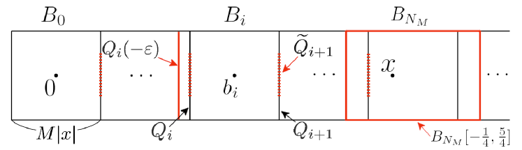
The structure of this section is as follows. First, we define several subsets of . These will be used to describe a number of events involving the simple random walk whose loop-erasure is . We provide some key estimates on the probabilities of these events in Lemmas 3.9 and Lemma 3.12. Finally, applying these results, we prove Proposition 3.6 at the end of this section.
We begin by defining “a tube connecting the origin and ”, which will consist of a number of boxes of side-length . To this end, for , let
Moreover, for and , define a sequence of vertices of by setting
| (20) |
for . Let us consider a rotation around the origin that aligns the -axis with the line through the origin and . We denote by and the images of and under this rotation, respectively. For , we let
| (21) |
be the tilted cube of side-length centered at , and we write for . For and with , also let
where
We also set
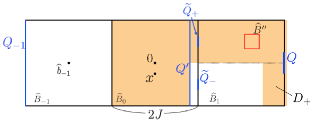
and note that, by definition, for all and . Observe that every is perpendicular to the line through the origin and , and that is the “left face” of the cube . Finally, we write
| (22) |
and set for convenience. See Figure 1 for a graphical representation of the situation.
In this section, it will be convenient to consider (recall that ) as a continuous curve in by linear interpolating between discrete time points, and thus we may assume that is defined for all non-negative real . If is a continuous path in and , we write
and also, for , we set , analogous to the notation of first hitting times for discrete paths (5).
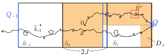
In order to obtain the lower bound (19), we consider events under which the LERW , started at the origin, travels through the “tube” until it hits . See Figure 2 for a graphical representation.
Definition 3.7.
We define the events , , as follows. Firstly,
For ,
Moreover,
and, for ,
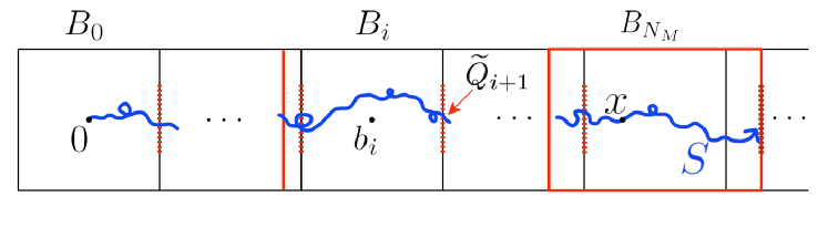
The first three conditions of the definition of each , , require that travels inside the “tube” and it exits each at a point which is not close to . Furthermore, the last condition in the definition of , the last two conditions in that of each , , and the third condition in that of control the range of backtracking of . Finally, the last condition in the definition of and events , guarantee that remains in .
Next, we define events that provide upper and lower bounds for the length of the loop-erasure of in each . For , let
| (23) |
and also set . We further define
| (24) |
Since is not necessarily a simple curve, and do not coincide in general. However, the restriction on the backtracking of on the events and a cut time argument (see Definition 3.10 and Definition 3.11 below) enable us to handle the difference between and . This will be discussed later, in the proof of Proposition 3.6.
We now define events upon which the length of is bounded above.
Definition 3.8.
For , the event is given by
and for , the event is given by
In the following lemma, we demonstrate that occurs with high conditional probability. Recall that was defined at (22).
Lemma 3.9.
For any , there exists a constant such that
| (25) |
uniformly in , , and .
Proof.
For , and , we have that
Moreover, by (9) and translation invariance, we have that there exists some constant such that
| (26) |
for all . For , the same argument yields that . Thus, it follows from (8) and (26) that
for some constant . By taking the sum over , we have that
| (27) |
The same argument also applies to the case , and thus we have
| (28) |
Similarly, for the case , recalling that was defined at (24), we have that
| (29) |
where we used the strong Markov inequality to obtain the last inequality. We will prove that later in this subsection, see (59).
Now we bound above the sum of the numerator of (29) over , separating into three cases depending on the location of .
- (i)
-
(ii)
For , a similar argument to case (i) yields that
-
(iii)
For , we have that
which gives
Thus, by (29), it holds that
| (30) |
Combining (27), (28) and (30) with Markov’s inequality, it holds that
for . By taking , we obtain (25). ∎
Now we will deal with events involving upon which the length of is bounded below and, at the same time, the gap between the lengths of and is bounded above. First, we define a special type of cut time of in each .
Definition 3.10.
A nice cut time in is a time satisfying the following conditions:
-
•
,
-
•
,
-
•
,
-
•
.
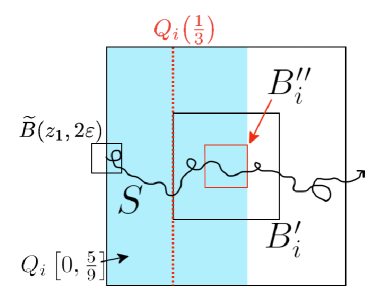
Second, let (respectively ) be the cube of side-length (respectively ) centered at whose faces are parallel to those of , i.e.
where and are as defined in (20) and (21), respectively. We denote by (respectively ) the “left (respectively right) face” of . See Figure 3.
Let be the first time that exits after it first entered . We define a set of local cut times of by
Finally, we define events as follows.
Definition 3.11.
For and ,
| (33) | ||||
where denotes the cardinality of set . Moreover, .
Note that, on the event , a local cut time satisfies
and thus holds.
Lemma 3.12.
Let be as defined above. Then there exists constants , , and such that
| (34) |
uniformly in and with , and .
Proof.
By the strong Markov property, we have that
| (37) | ||||
| (40) | ||||
where the infima are taken over , , and (see (21) for the definition of ).
First we estimate the conditional probability of . Recall that denotes the Euclidean ball of radius with center point . We consider the event of up to the first exit time of the small box . Let and . Then
| (44) | |||||
If we take sufficiently large, then the second and third terms on the right-hand side of (44) are bounded below by some small constant, while it follows from [21, equation (1)] that the first term is bounded below by some universal constant. Thus, we have
| (45) |
for some constant .
Second we consider the conditional probability of . By (7), there exists some universal constant such that
for . It follows from (9) that
uniformly in . Thus we have that
| (46) |
for some constant and sufficiently small .
We will next derive a lower bound for by applying the second moment method. We consider the ball and two independent simple random walks and with starting point . Let for . We define two events of and as follows:
Let us denote by the joint distribution of and . By [7, Lemma 3.2], we have
| (50) |
while it follows from [20, equation (3.2)] that for some constant . On , without loss of generality, we suppose that . Let
where (respectively ) is the line segment between the points and (or between and , respectively). (See Figure 4 for a depiction of .)
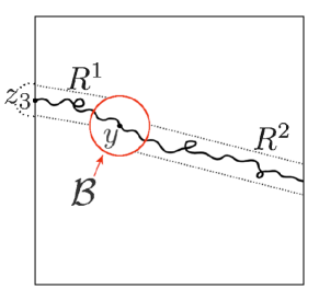
Since is comparable to , we have that
for some constant . Moreover, by the strong Markov property and (8),
| (51) |
for some constant . By the strong Markov property, we bound from below the expectation of on the event by
| (52) |
On the other hand, the first and second moment of is bounded above as follows. Since for and ,
| (53) |
| (54) |
where and depend only on . Now, for , we have that
From this, since , the Cauchy-Schwarz inequality yields
By substituting (52), (53) and (54) into the above estimate, we obtain that
| (55) |
We are now ready to prove Proposition 3.6. Recall that , and were defined in Definitions 3.7, 3.8 and 3.11, respectively. Let
and
Proof of Proposition 3.6.
We will first demonstrate that the bound , as appears in the probability on the left-hand side of (19), holds on . Suppose that occurs. By the definition of , ,
holds. Thus and . Let be a nice cut time of in (see Definition 3.10), and recall that and are as defined in (23) and (24), respectively. Let
Then we have that
| (56) |
and also
for , where we have applied (56) for the inclusion. Furthermore,
Thus, by induction, it follows that
Note that, on , is a cut time of the path , and thus . By the definition of and (see Definitions 3.8 and 3.11, respectively), we have that
on . Hence choosing suitably large gives the desired bound on .
Consequently, to complete the proof, it will be enough to show that is bounded below by the right-hand side of (19). By Lemma 3.12, there exist constants such that for . Moreover, by Lemma 3.9, there exists a constant such that for . Thus we have
| (57) |
| (58) |
As already noted in the proof of Lemma 3.9, we also have that
| (59) |
for all , and a similar bound holds for . And, repeating a similar argument to the lower bound for from the proof of Lemma 3.12, from (50) to (51) we have that
where is adjusted if necessary. By combining these estimates on with (57) and (58), we obtain that
Furthermore, similarly to the case with , it holds that
and it follows from (7) that
for some constant . Finally, by the strong Markov property, we have that
where the third inequality holds simply because . ∎
3.4 Lower bound for
We now turn to the proof of the lower bound of Proposition 3.1 with . In particular, we will establish the following.
Proposition 3.13.
There exist constants such that for every and ,
As in the previous section, the basic strategy involves the construction of a set of particular realisations of that we can show occurs with suitably high probability. To do this, we will use a certain reversibility property of simple random walk, as is set out in the next lemma. In the statement of this, for a finite path , we write for its time reversal.
Lemma 3.14.
Let , , and write , for independent simple random walks in started at , , respectively. Moreover, write , ,
It then holds that
| (60) |
and, denoting the set above ,
| (61) |
Proof.
In order to explain our application of the previous result, we need to introduce some notation. First, let and . Moreover, set for some that will be determined later, and, for , write and
which represent adjacent cubes of side length . We also introduce the following smaller cubes centred at ,
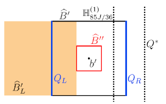
Note that . See Figure 5 for a sketch showing the cubes , , and , as well as some of the other objects that we now define. In particular, we introduce a collection of surfaces:
the hyperplane , where for and , we denote
(see Figure 7 below for the location of in particular); and also the following regions:
We highlight that is shown as the shaded region on Figure 5.
Roughly speaking, to establish the main result of this section, we will show that, with high enough probability, the loop-erased random walk passes from 0 to (somewhere close to) through , spending a suitable time in on the way, before returning to through , and then escapes to via . To make this precise, we will consider an event based on the simple random walk started from ; see Figure 6. Controlling the probability of this will involve an appeal to Lemma 3.14, through which we obtain a bound that depends on three independent random walks, one started from and two started from (see Lemma 3.15 below).
Concerning notation, as in the statement of Lemma 3.14, for each , we will write for a simple random walk started from . We assume that the elements of the collection are independent. We moreover write for an independent copy of . We also set
and . A particularly important point in the argument that follows is given by
i.e. the location where hits , which is defined when . Additionally, we introduce
and, to describe a collection of local cut points for a path ,
The following result gives the key decomposition of the simple random walk underlying that we will consider later in the section. It already takes into account the time-reversal property of Lemma 3.14. We will break the complicated event that appears in the statement into several more convenient pieces below.
Lemma 3.15.
In the setting described above, is bounded below by the probability of the following event:
Proof.
Clearly,
is a subset of the event . Now, conditioning on the value of and applying the strong Markov property at times and , we have that the probability of the above event is equal to
Applying Lemma 3.14, we can replace and in the above expression by and , respectively, where , are defined as in the statement of that result. Since , it holds that . Consequently, we obtain that the above sum is bounded below by
and replacing the sum with a union inside the probability completes the proof. ∎
Now, we will rewrite the event we defined in the statement of Lemma 3.15 as the intersection of various smaller events concerning , and . For convenience, we will write
in the remainder of this subsection. We moreover define the event by setting
On , the paths , and do not have an intersection and move along the different courses until they first exit the union of and .
Next, we will define some events that restrict the behavior of after . First, recall that and . We define the “left” and “right” faces of by
Moreover, we define a subset of by setting
See Figure 7. Then, writing and , let
| (62) | ||||
| (65) | ||||
| (66) |
and set . In particular, on the event , we have the existence of cut points of contained in . Finally let
be events that restrict the regions where and can explore, respectively.
We continue by checking the local cut points that we construct on the event are cut points of the loop-erasure of . Note that on the event , it follows from the definition of and that
Moreover, on the event , we have that
-
•
,
-
•
,
-
•
.
The first and second statements follow from the definitions of and , respectively, while the third statement is derived from the definitions of and (recall the definitions of the sets defined above, which are also shown in Figure 7). From these statements, we immediately conclude that
For the rest of the path , the definition of implies that
Combining the preceding three statements, we see that, on ,
where we recall that is be the last exit time of by (we assume here that is stopped at ). Thus, the local cut points of the event are indeed cut points of the loop-erasure of and the probability of the event we defined in the statement of Lemma 3.15 is bounded below by
In what follows, we will bound below this probability below. To start with, we will prove that , and do not have an intersection and are separated in a cube with positive probability. Let . We define the event by setting
and let be given by
where here is the Euclidean distance, i.e. is the minimum of the distance between the point from which either , or exits and the union of the other two paths up to their exit times.
Lemma 3.16.
There exists and such that: for all ,
Proof.
For readability, we assume that . (Other cases will follow by a small modification of the argument.) We follow the idea of [7, Lemma 3.2]. Let and . We define the event by setting
where will be fixed later. Then we have .
We will show that the probability that , and do not intersect before they first exit from conditioned on is bounded above by arbitrarily small by taking sufficiently large. Let be the number of intersections of , and , i.e.
Then by the Markov inequality,
| (67) |
for some , , where we applied the Gaussian estimate for the off-diagonal heat kernel of the simple random walk on for the last inequality (see (1)). Since , the right-hand side of (67) converges to 0 as .
Our next step is to construct subsets where each simple random walk path is constrained to move until it first exits from . We define by
the subsets of the left and right face of in the direction of -axis, respectively, and by
the subset of the upper face of in the direction of -axis. Let
and . It is an elementary exercise to check that there exists some such that holds uniformly in and . Note that on the event , it holds that
so that . Similarly, the same bound holds for and . Thus we have on the event in question. Finally, by taking large so that , we obtain that
which completes the proof. ∎
We are now ready to complete the proof of the main result of this subsection.
Proof of Proposition 3.13.
For any , we have that
Now, by the argument used to prove Proposition 3.2, we have that
Thus, by taking suitably large, and applying Lemma 3.15 and the argument above Lemma 3.16, to complete the proof it suffices to prove that
for some constant .
First, we derive an estimate for from the result of Lemma 3.16. We take large so that . We then define the event by setting
Recall the definition of the events and and the random variable from the proof of Lemma 3.16. It is straightforward to check that if we take , then
Moreover, by the strong Markov property and the approximation to Brownian motion, there exists some constant such that , uniformly in and . By Lemma 3.16, we thus obtain that
| (68) |
Next we estimate . It follows from the strong Markov property that
where , and are as defined in (62), (65) and (66), respectively. Thus it suffices to bound from below the right-hand side of the above inequality. We begin with a lower bound for . By the gambler’s ruin estimate (9), we have that for some universal constant . Next, applying a similar argument to that used to obtain (55) in the proof of Lemma 3.12 and the strong Markov property, we obtain that . Finally, again by (9) and the strong Markov property, we have that . Since does not depend on , we can conclude that
| (69) |
By the independence of and and the strong Markov property, we also have that
Let and . Again by the strong Markov property,
| (70) |
We will give lower bounds for the two probabilities in the right-hand side. Let be the piecewise linear curve that runs from in the direction of until its second coordinate reaches , and then runs along the line from that point to . Similarly to (51) in Lemma 3.12, we obtain that
| (71) |
uniformly in and for some . Furthermore, we have that
where we applied (8) with to the last inequality. Thus, by increasing the value of the constant in if necessary, we have that
| (72) |
for some uniform constant . Plugging (71) and (72) into (70) yields that
| (73) |
Now we will give a lower bound for . Recall that . By the strong Markov property and the definition of the events , and , we have that
From this, it is an easy application of (7) to deduce that
| (74) |
for some universal constant .
4 Heat kernel estimates for the associated random walk
The aim of this section is to prove Theorem 1.3. As explained in the introduction, the main input concerning the loop-erased random walk will be Theorem 1.1. To estimate using the decomposition at (4), we also require control over , where in this section is always the infinite LERW started from 0. Since the structure of the graph is simply that of equipped with nearest-neighbour bonds, we have the obvious identity
where gives the transition probabilities of the continuous-time simple random walk on with unit mean holding times. For this, we have the following estimates from [3]. (We note that although the result we will cite in [3] is stated for the simple random walk on , it is easy to adapt to apply to the half-space .)
Lemma 4.1.
For any , there exist constants such that for every and ,
and also
Moreover, for and , we have that
Proof.
From [3, Theorem 6.28(b)], we obtain the relevant bounds for . Moreover, the bounds for , , follow from [3, Theorem 6.28(d)]. As for , , we can apply [3, Theorem 6.28(c)] to deduce that is bounded above and below by an expression of the form:
This can be bounded above and below by an expression of the form , and that in turn by , uniformly over the range of and considered. This completes the proof of the first two inequalities in the statement of the lemma. The third inequality is given by again applying [3, Theorem 6.28(c)]. ∎
We are now ready to proceed with the proof of Theorem 1.3.
Proof of Theorem 1.3.
We next suppose . In this case, applying Lemma 4.1 with , we find that
| (75) | |||||
Now, the second sum here is readily bounded as follows:
Moreover, since we are assuming , the final expression is readily bounded above by one of the form
Thus, to complete the proof of upper bound in the statement of Theorem 1.3, it remains to derive a similar bound for the first sum on the right-hand side at (75). For this, we have that
| (76) | |||||
where we have applied Theorem 1.1 for the second inequality. To bound the integral, we first note that, for any , it is possible to find a constant such that for all . In particular, choosing , this implies that
Hence, applying this estimate and the change of variable , we obtain
| (77) | |||||
Now, let , and note that this is a function that has a unique minimum on such that . Thus, for , the remaining integral above is estimated as follows:
Putting this together with (76) and (77), we deduce the desired result in the range . If , then we follow a simpler argument to deduce:
where we have applied Lemma 4.1 for the first inequality, and (8) for the third. This is enough to establish that the upper bound of Theorem 1.3 holds in this case as well.
For the lower bound when , we follow a similar argument to the upper bound, but with additional care about the range of summation/integration. In what follows, we set , where, here and for the rest of the proof, , are the constants of Theorem 1.1. Clearly, we can assume that , so that . Recall that we are also assuming , and without loss of generality, we may suppose . Applying the bounds of Lemma 4.1 with given by
we deduce that
where for the second inequality, we have applied that
and the observation that each can appear in at most two of the intervals . (We also note that our choice of ensures , and so the sum is non-empty.) Consequently, applying Theorem 1.1 with , we find that
where we have used that to obtain the bottom limit of the integral, and the choice of to obtain the top one. Making the change of variable yields a lower bound for the integral of
and, since , our choice of implies that this is bounded below by
Hence, if , we can put the pieces together to find that
as required. Finally, for , continuing to suppose that is the constant of Theorem 1.1, we have that
where we have applied Lemma 4.1 with for the second inequality, that for the third, and Theorem 1.1 for the final one. ∎
Acknowledgements
DC was supported by JSPS Grant-in-Aid for Scientific Research (C) 19K03540 and the Research Institute for Mathematical Sciences, an International Joint Usage/Research Center located in Kyoto University. DS was supported by JSPS Grant-in-Aid for Scientific Research (C) 22K03336, JSPS Grant-in-Aid for Scientific Research (B) 22H01128 and 21H00989. SW is supported by JST, the Establishment of University Fellowships Towards the Creation of Science Technology Innovation, Grant Number JPMJFS2123.
References
- [1] O. Angel, D. A. Croydon, S. Hernandez-Torres, and D. Shiraishi, Scaling limits of the three-dimensional uniform spanning tree and associated random walk, Ann. Probab. 49 (2021), no. 6, 3032–3105.
- [2] L. Avena, E. Bolthausen, and C. Ritzmann, A local CLT for convolution equations with an application to weakly self-avoiding random walks, Ann. Probab. 44 (2016), no. 1, 206–234.
- [3] M. T. Barlow, Random walks and heat kernels on graphs, London Mathematical Society Lecture Note Series, vol. 438, Cambridge University Press, Cambridge, 2017.
- [4] M. T. Barlow and R. F. Bass, The construction of Brownian motion on the Sierpiński carpet, Ann. Inst. H. Poincaré Probab. Statist. 25 (1989), no. 3, 225–257.
- [5] M. T. Barlow, D. A. Croydon, and T. Kumagai, Subsequential scaling limits of simple random walk on the two-dimensional uniform spanning tree, Ann. Probab. 45 (2017), no. 1, 4–55.
- [6] , Quenched and averaged tails of the heat kernel of the two-dimensional uniform spanning tree, Probab. Theory Related Fields 181 (2021), no. 1-3, 57–111.
- [7] M. T. Barlow and A. A. Járai, Geometry of uniform spanning forest components in high dimensions, Canad. J. Math. 71 (2019), no. 6, 1297–1321.
- [8] G. Ben Arous, M. Cabezas, and A. Fribergh, Scaling limit for the ant in a simple high-dimensional labyrinth, Probab. Theory Related Fields 174 (2019), no. 1-2, 553–646.
- [9] , Scaling limit for the ant in high-dimensional labyrinths, Comm. Pure Appl. Math. 72 (2019), no. 4, 669–763.
- [10] D. A. Croydon, Random walk on the range of random walk, J. Stat. Phys. 136 (2009), no. 2, 349–372.
- [11] D. A. Croydon and D. Shiraishi, Scaling limit for random walk on the range of random walk in four dimensions, Ann. Inst. Henri Poincaré Probab. Stat. 59 (2023), no. 1, 166–184.
- [12] R. D. DeBlassie, Iterated Brownian motion in an open set, Ann. Appl. Probab. 14 (2004), no. 3, 1529–1558.
- [13] M. D. Donsker, An invariance principle for certain probability limit theorems, Mem. Amer. Math. Soc. 6 (1951), 12.
- [14] T. Hara and G. Slade, The lace expansion for self-avoiding walk in five or more dimensions, Rev. Math. Phys. 4 (1992), no. 2, 235–327.
- [15] , Self-avoiding walk in five or more dimensions. I. The critical behaviour, Comm. Math. Phys. 147 (1992), no. 1, 101–136.
- [16] M. Heydenreich, R. van der Hofstad, and T. Hulshof, Random walk on the high-dimensional IIC, Comm. Math. Phys. 329 (2014), no. 1, 57–115.
- [17] G. Kozma and A. Nachmias, The Alexander-Orbach conjecture holds in high dimensions, Invent. Math. 178 (2009), no. 3, 635–654.
- [18] T. Kumagai, Random walks on disordered media and their scaling limits, Lecture Notes in Mathematics, vol. 2101, Springer, Cham, 2014, Lecture notes from the 40th Probability Summer School held in Saint-Flour, 2010, École d’Été de Probabilités de Saint-Flour. [Saint-Flour Probability Summer School].
- [19] G. F. Lawler, A self-avoiding random walk, Duke Math. J. 47 (1980), no. 3, 655–693.
- [20] , Intersections of random walks, Probability and its Applications, Birkhäuser Boston, Inc., Boston, MA, 1991.
- [21] , Cut times for simple random walk, Electron. J. Probab. 1 (1996), no. 13, approx. 24 pp.
- [22] G. F. Lawler and V. Limic, Random walk: a modern introduction, Cambridge Studies in Advanced Mathematics, vol. 123, Cambridge University Press, Cambridge, 2010.
- [23] R. van der Hofstad and G. Slade, A generalised inductive approach to the lace expansion, Probab. Theory Related Fields 122 (2002), no. 3, 389–430.
- [24] , The lace expansion on a tree with application to networks of self-avoiding walks, Adv. in Appl. Math. 30 (2003), no. 3, 471–528.