Anisotropic scattering caused by apical oxygen vacancies in thin films of overdoped high-temperature cuprate superconductors
Abstract
There is a hot debate on the anomalous behavior of superfluid density in overdoped La2-xSrxCuO4 films in recent years. The linear drop of at low temperatures implies the superconductors are clean, but the linear scaling between (in the zero temperature limit) and the transition temperature is a hallmark of the dirty limit in the Bardeen-Cooper-Schrieffer (BCS) framework [I. Bozovic et al., Nature 536, 309 (2016)]. This dichotomy motivated exotic theories beyond the standard BCS theory. We show, however, that such a dichotomy can be reconciled naturally by the role of increasing anisotropic scattering caused by the apical oxygen vacancies. Furthermore, the anisotropic scattering also explains the “missing” Drude weight upon doping in the optical conductivity, as reported in the THz experiment [F. Mahmood et al., Phys. Rev. Lett. 122, 027003 (2019)]. Therefore, the overdoped cuprates can actually be described consistently by the -wave BCS theory with the unique anisotropic scattering.
Introduction.— For a long time, the overdoped cuprate superconductors were believed to be described quite well by the Bardeen-Cooper-Schrieffer (BCS) theory Lee et al. (2006); Keimer et al. (2015). However, in 2016, such a belief was challenged by the measurement of the superfluid density using mutual inductance technique on a large amount of high quality overdoped La2-xSrxCuO4 (LSCO) films Božović et al. (2016). Two seemingly contradicting results were reported: and where is the zero temperature value of and is the transition temperature. Within the conventional BCS theory, the former scaling law indicates the d-wave superconductors are very clean, but the latter is a result of dirty BCS superconductors Abrikosov et al. (1963). This dichotomy regarding the dirtiness/cleanness of the overdoped cuprates motivated exotic theoretical investigations Božović et al. (2019); Zaanen (2016); Herman and Hlubina (2018); Fu et al. (2018); Wang (2018); Goutéraux and Mefford (2020); Phillips et al. (2020); Li et al. (2021).
The superfluid density has also been measured by THz optical conductivity experiment Mahmood et al. (2019), and is quantitatively consistent with the mutual inductance measurement Božović et al. (2016). In the meantime, the Drude fitting of the optical conductivity indicates the dirty limit Lee-Hone et al. (2017, 2018). So the same dichotomy also exists in optical measurements. Moreover, as yet another puzzle, should be identical to, but is fitted to be significantly smaller than the dc conductivity Mahmood et al. (2019). This superficial loss of Drude weight seems to increase with overdoping.
In this Letter, we propose a scenario to resolve all of the above mysteries. We realize that in addition to the conventional isotropic scattering rate Lee-Hone et al. (2017, 2018), the apical oxygen vacancies cause an anisotropic scattering rate , with the azimuthal angle of the quasiparticle momentum relative to the antinodal direction. Since the low-energy nodal quasiparticles are barely affected by , they reduce the superfluid density linearly in temperature if in addition . But the total scattering rate determines the typical behavior in the dirty limit. Meanwhile, the strong anisotropy in causes a continuous distribution of Lorentzian components in , so that would be underestimated by extrapolation from finite frequencies if a single isotropic scattering rate were assumed instead Mahmood et al. (2019).
Oxygen vacancies and “cold spot” model.— From both early Torrance et al. (1988); Sato et al. (2000) and recent Kim et al. (2017) studies, apical oxygen vacancies were found to be an important factor to prevent obtaining (high-quality) overdoped LSCO samples. Therefore, the effect of apical oxygen vacancies deserves study in overdoped cuprates carefully. This is another motivation of the present work.
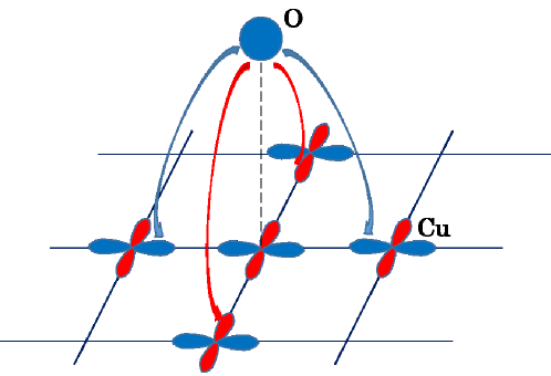
In Fig. 1, we plot a configuration of one apical oxygen atom above the CuO2-plane (only Cu-sites plotted). Notice that since the carriers have -like orbital content Zhang and Rice (1988), there is no coupling between the oxygen and the -orbital just below it. Therefore, the leading couplings are with the next nearest neighboring sites, giving the hopping integrals switching signs alternatively, as shown in Fig. 1. First, if there is no oxygen vacancy, the second order process of these out-of-plane hoppings gives an additional band dispersion where with and the hopping amplitude and energy level distance between the apical oxygen and orbitals Xiang and Wheatley (1996). Such a dispersion has already enters the carrier band. Next, we consider one oxygen vacancy at the origin. Relative to the uniform background, the vacancy now leads to an additional term where for and denotes spin, which gives rise to the following scattering Hamiltonian
| (1) |
where and are momentums, and is the number of copper atoms. Since the oxygen vacancies are out-of-plane and only couple to next nearest neighboring -orbitals, the scattering strength is anticipated to be small. Under the Born approximation Abrikosov et al. (1963), gives a scattering rate . For analytical convenience but without loss of qualitative physics, throughout this work, we further assume circular fermi surface and use wide band approximation, so that the scattering rate is only angle-dependent, i.e.
| (2) |
where we have added the isotropic scattering rate arising from, e.g., in-plane impurities. In the following calculations, and are our model parameters. In fact, this kind of scattering rate has been proposed to explain the transport phenomena in underdoped cuprates, called “cold spot” model Ioffe and Millis (1998), where the -term is attributed to the pair fluctuations or interaction effects, which hence is expected to decrease upon doing. But here, in our case, the -term is caused by oxygen vacancies and should increase upon doping, according to both early Torrance et al. (1988); Sato et al. (2000) and recent Kim et al. (2017) experiments.
We now look at the effect of the anisotropic scattering on single particle excitations. By choosing the d-wave pairing function and fixing , we calculate the density of states (DOS) , where is the partial DOS (PDOS) given by
| (3) |
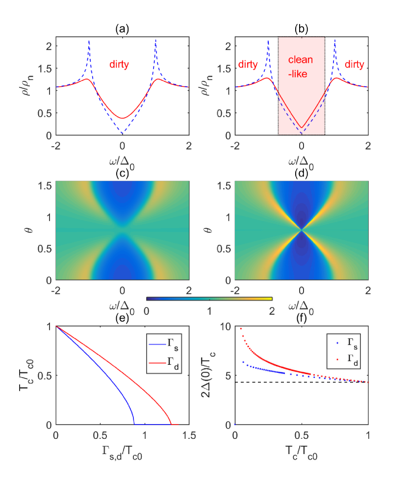
where is the normal state DOS and . and are plotted in Fig. 2(a)-(d). In the calculations, we perform the integrals over and using standard numerical integral technique. Fig. 2(a) is the typical behavior of the conventional d-wave superconductor with isotropic scattering rate: zero energy cusp and coherence peak are both smeared out by isotropic scattering rate. Differently, the -scattering shown in Fig. 2(b) only suppresses the coherence peak but does not change the zero energy cusp, as a result of the vanishing of scattering rate for nodal quasiparticles. Accordingly, we can divide the energy space into two regions: lower energy “clean” one and higher energy “dirty” one. The above picture is also seen clearly from the PDOS in Fig. 2(d), where the spectral becomes smeared out for high energy quasiparticles (near the antinodes) but remains sharp for low energy ones (near the nodes).
The dirty BCS theory for d-wave superconductors Alloul et al. (2009) is a direct generalization of the Abrikosov-Gor’kov (AG) theory Abrikosov and Gor’kov (1961), since the potential scattering here causes pair-breaking which is similar to the magnetic impurities in s-wave superconductors. The gap is determined by the self-consistent equation
| (4) |
where is the BCS coupling constant, the Matsubara frequency, and the d-wave form factor. 111Exactly speaking, the frequency summation should be bounded with a soft-cutoff (with the form of a boson propagator) instead of the hard-cutoff used here. However, only the latter can be mapped to the momentum cutoff strategy as in the BCS treatment. In numerical calculations, we use and , which gives for clean superconductors (with this setup, is taken as the energy unit). By letting , we obtain the generalized -formula
| (5) |
where is the digamma function. The results of vs and are shown in Fig. 2(e). A stronger is needed to kill superconductivity as the low energy excitations are less affected. In Fig. 2(f), we show the results of . It is interesting to find that the anisotropic scattering drives the ratio farther away from the BCS prediction in the clean limit to values as large as . In the literature, a large gap- ratio is often taken as an indication of strong coupling superconductivity. Here, the anisotropic scattering gives another interpretation.
Superfluid density.— After recognizing the clean-dirty dichotomy caused by oxygen vacancies at the single particle level, we turn to discuss the superfluid density, which can be obtained as Coleman (2015)
| (6) |
where is the Fermi velocity. Here, the current vertex correction can be proven to vanish in the non-crossing approximation as a result of the factorized scattering potential (Eq. 1), as shown in the Supplementary Material sm . In Fig. 6(a) and (b), vs is plotted for pure and scatterings, respectively. The most obvious difference is that any nonzero causes power law temperature dependence of , but preserves the linear dependence as in the clean limit. This is already anticipated from the DOS feature in Fig. 2(b) because the normal fluid density is roughly determined by quasiparticles and thus satisfies , leaving the superfluid density satisfying .
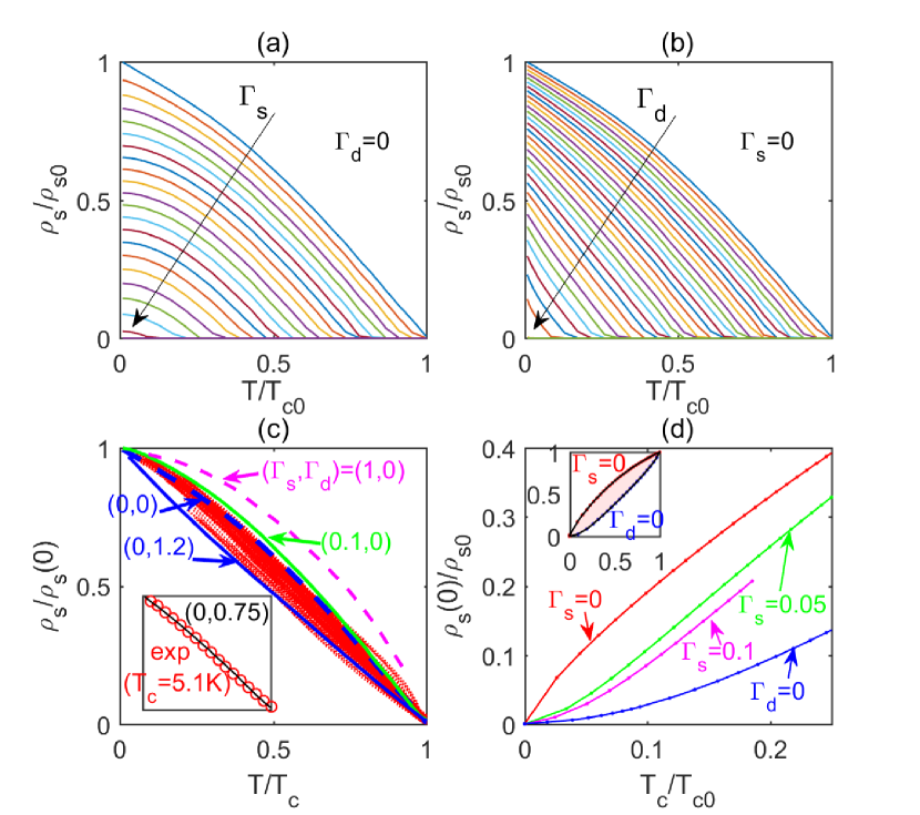
In real materials, both and are expected to coexist. In order to make quantitative comparisons with the experiment, we renormalize and by and , respectively, as shown in Fig. 6(c). We have superposed the experimental data of all samples with ranging from to K Božović et al. (2016), shown as the red dots. Four typical theoretical curves are plotted: , , , and . As can be seen, almost all the experimental data reside within the region enclosed by the curves of (green line) and (blue line), while if is large and dominant, as the -line shows, the renormalized - curve bends more significantly, which is at odds with the experimental data. These observations indicate the more important role of . As an example, the experimental data (open circles) with K are shown in the inset, which is clearly very linear. We can fit the data with pure (line) quite well.
Another key observation of the experiment Božović et al. (2016) is the linear relationship between vs . To see that, we plot our results in Fig. 6(d). Pure and scatterings correspond to blue and red curves, which enclose the physical region (shaded region in the inset), in which is always roughly proportional to although not exactly. Therefore, this is a hallmark of the dirty BCS superconductors regardless of isotropic () or anisotropic () scatterings. Furthermore, we have also fix and and tune to suppress . Both of them show the bending behavior near , showing much better behavior than the separate scattering cases in view of the experimental data .
Optical conductivity.— From the Kubo formula, the optical conductivity can be obtained as Hirschfeld et al. (1989)
| (7) |
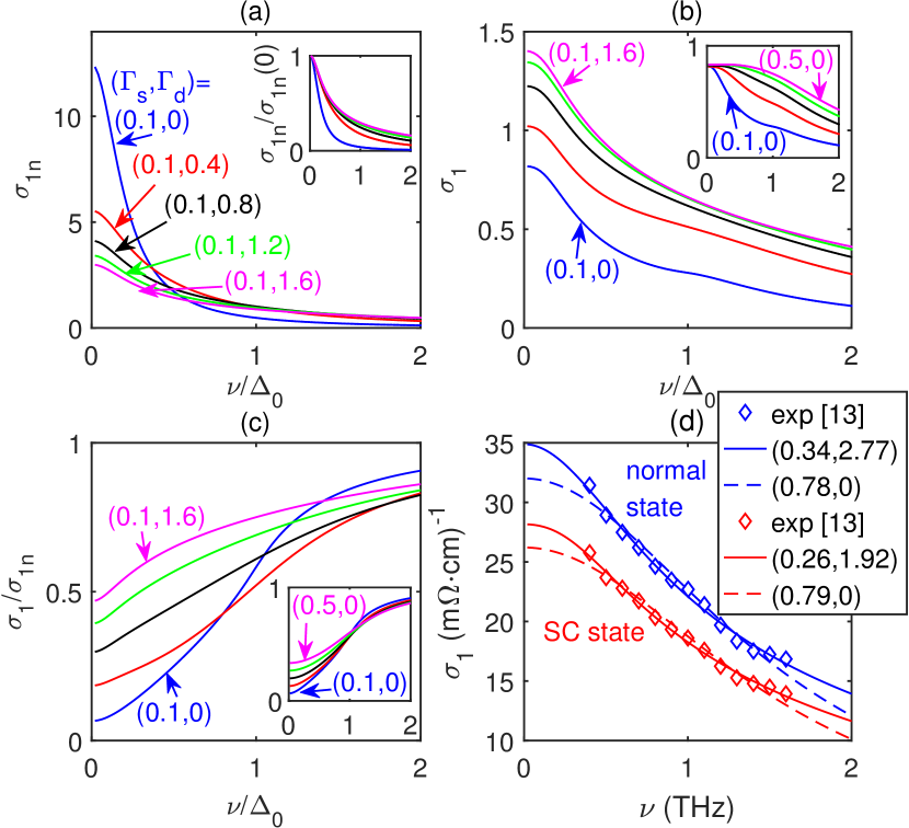
where is the Fermi distribution function, is the Green’s function in the Nambu space: with the identity and Pauli matrices. By numerical calculations, we obtain the frequency dependence of in both normal and superconducting states (with as the energy unit), as shown in Fig. 7(a) and (b), respectively. In the normal state, as increases, becomes more and more broadened to show long tail behavior. This is an important feature obtained in the “cold spot” model Ioffe and Millis (1998). In the superconducting state, a nonzero breaks the universal conductivity Lee (1993), which applies only in the case of pure scattering as shown in the inset of Fig. 7(b). Furthermore, we renormalize the superconducting state by the normal state value to obtain the results shown in Fig. 7(c). The resulted curves show similar behavior to the DOS at low frequencies: nearly linear -dependence if dominates which is quite different from the case of pure scattering (inset) with quadratic -dependence. This can be used to examine the types of scattering in future experiments.
The most obvious feature when dominates is the behavior of is no longer a simple Lorentian-like Drude peak (as in the case of isotropic scattering), since the quasiparticles experience angle dependent scattering rates. In fact, the conductivity should be an integration over a continuous distribution of Lorentzian components. Since the Lorentzian is sharper and higher for smaller scattering rates, the overall line shape of should be steeper as the frequency approaches zero. Therefore, if the finite frequency data are used to perform the fit to a single Lorentzian-like Drude peak, as in the THz experiment, the extrapolated value of will be lower than the actual one, leading to superficial “missing” of the Drude weight. As an example, in Fig. 7(d) we fit the experimental data with K (symbols) in both normal (blue) and superconducting (red) states Mahmood et al. (2019). The best fits with only (dashed lines) are found to underestimate and the spectral weight, as compared to the result with both and (solid lines). Since the pairing gap is not available in the experiment, we take it also as a parameter, and the fitted value is THz. More systematic fitting for a series of overdoped samples can be found in the Supplemental Material sm , which supports our main point that apical oxygen vacancy increases with overdoping, leading to larger scattering.
Summary and discussions.— In summary, we have found that the apical oxygen vacancies give rise to an anisotropic scattering rate which causes a clean-dirty dichotomy for low-high energy excitations. This provides a natural explanation of the anomalous behavior of the superfluid density and THz optical conductivity in the experiments. Therefore, we conclude that the superconducting states of overdoped cuprates are still captured by the BCS theory, as long as the anisotropic scattering rate is adequately considered.
Finally, we make some remarks. (1) In this work, we have omitted many material-dependent details (such as specific tight-binding models, pairing interactions and interaction effects) in order to obtain universal results. The doping dependence enters the problem via the scattering rate , which increases with doping. (2) The anisotropic scattering rate has been reported in angle-dependent magnetoresistivity experiments in Nd-LSCO Grissonnanche et al. (2021) and Tl2Ba2CuO6+δ Abdel-Jawad et al. (2006). But to the best of our knowledge, there has not been such report in overdoped LSCO films. A systematic study of the anisotropic scattering rate can check our model and finally answer the question on whether overdoped cuprates are dirty BCS superconductors or not. (3) Our prediction suggests that it is necessary to extend the optical measurements down to even lower frequency (e.g. GHz) in order to obtain accurate behavior of the optical conductivity. (4) About superfluid density, there are two other kinds of scalings reported in literature: Uemura’s law Uemura et al. (1989) and Homes’ law Homes et al. (2004). The former is obtained in underdoped cuprates, where phase fluctuations are very strong and cannot be neglected. Emery and Kivelson (1995). On the other hand, Homes’ law can be explained by dirty BCS superconductors with pair-preserving impurities only Abrikosov et al. (1963); Kogan (2013). Here, in the overdoped LSCO films, the oxygen vacancies are pair-breaking, hence Homes’ law does not apply. (5) Recently, the apical oxygen vacancies have also been observed in optimally doped YBa2Cu3O7-x Hartman et al. (2019). Then, according to our study, at low frequency should be non-standard Drude-like, which may be consistent with the early microwave experiment Turner et al. (2003). Furthermore, if the apical oxygen vacancies are widely present in different families of cuprates, then the effect of scattering should be considered carefully in future studies.
D. W. thanks Congjun Wu, Qi Zhang, Tao Li, Yuan Wan for helpful discussions during the past few years. D. W. also acknowledges Ivan Bozovic for his encouragement on studying their experiments. This work is supported by National Natural Science Foundation of China (under Grant Nos. 11874205, 11574134, and 12074181), National Key Projects for Research and Development of China (Grant No.2021YFA1400400), Fundamental Research Funds for the Central Universities (Grant No. 020414380185), and Natural Science Foundation of Jiangsu Province (No. BK20200007).
References
- Lee et al. (2006) P. A. Lee, N. Nagaosa, and X.-G. Wen, Rev. Mod. Phys. 78, 17 (2006).
- Keimer et al. (2015) B. Keimer, S. A. Kivelson, M. R. Norman, S. Uchida, and J. Zaanen, Nature 518, 179 (2015).
- Božović et al. (2016) I. Božović, X. He, J. Wu, and A. T. Bollinger, Nature 536, 309 (2016).
- Abrikosov et al. (1963) A. A. Abrikosov, L. Gorkov, and I. E. Dzialoshinskii, Methods of quantum field theory in statistical physics (NJ, Prentice-Hall, 1963).
- Božović et al. (2019) I. Božović, J. Wu, X. He, and A. Bollinger, Physica C: Superconductivity and its Applications 558, 30 (2019).
- Zaanen (2016) J. Zaanen, Nature 536, 282 (2016).
- Herman and Hlubina (2018) F. Herman and R. Hlubina, Phys. Rev. B 97, 014517 (2018).
- Fu et al. (2018) W. Fu, Y. Gu, S. Sachdev, and G. Tarnopolsky, Phys. Rev. B 98, 075150 (2018).
- Wang (2018) D. Wang, Chin. Phys. B 27, 057401 (2018).
- Goutéraux and Mefford (2020) B. Goutéraux and E. Mefford, Phys. Rev. Lett. 124, 161604 (2020).
- Phillips et al. (2020) P. W. Phillips, L. Yeo, and E. W. Huang, Nat. Phys. 16, 1175 (2020).
- Li et al. (2021) Z.-X. Li, S. A. Kivelson, and D.-H. Lee, npj Quantum Mater. 6, 36 (2021).
- Mahmood et al. (2019) F. Mahmood, X. He, I. Božović, and N. P. Armitage, Phys. Rev. Lett. 122, 027003 (2019).
- Lee-Hone et al. (2017) N. R. Lee-Hone, J. S. Dodge, and D. M. Broun, Phys. Rev. B 96, 024501 (2017).
- Lee-Hone et al. (2018) N. R. Lee-Hone, V. Mishra, D. M. Broun, and P. J. Hirschfeld, Phys. Rev. B 98, 054506 (2018).
- Torrance et al. (1988) J. B. Torrance, Y. Tokura, A. I. Nazzal, A. Bezinge, T. C. Huang, and S. S. P. Parkin, Phys. Rev. Lett. 61, 1127 (1988).
- Sato et al. (2000) H. Sato, A. Tsukada, M. Naito, and A. Matsuda, Phys. Rev. B 61, 12447 (2000).
- Kim et al. (2017) G. Kim, G. Christiani, G. Logvenov, S. Choi, H.-H. Kim, M. Minola, and B. Keimer, Phys. Rev. Materials 1, 054801 (2017).
- Zhang and Rice (1988) F. C. Zhang and T. M. Rice, Phys. Rev. B 37, 3759 (1988).
- Xiang and Wheatley (1996) T. Xiang and J. M. Wheatley, Phys. Rev. Lett. 77, 4632 (1996).
- Ioffe and Millis (1998) L. B. Ioffe and A. J. Millis, Phys. Rev. B 58, 11631 (1998).
- Alloul et al. (2009) H. Alloul, J. Bobroff, M. Gabay, and P. Hirschfeld, Rev. Mod. Phys. 81, 45 (2009).
- Abrikosov and Gor’kov (1961) A. A. Abrikosov and L. P. Gor’kov, Sov. Phys. JETP 12, 1243 (1961).
- Note (1) Exactly speaking, the frequency summation should be bounded with a soft-cutoff (with the form of a boson propagator) instead of the hard-cutoff used here. However, only the latter can be mapped to the momentum cutoff strategy as in the BCS treatment.
- Coleman (2015) P. Coleman, Introduction to Many-Body Physics (Cambridge University Press, 2015).
- (26) See Supplemental Material [url] for calculation details and further discussions, which includes Refs. Abrikosov et al. (1963); Abrikosov and Gor’kov (1961); Coleman (2015); Mahmood et al. (2019); Kramer et al. (2019); Kim et al. (2017); Lee and Ramakrishnan (1985); Božović et al. (2016).
- Hirschfeld et al. (1989) P. J. Hirschfeld, P. Wölfle, J. A. Sauls, D. Einzel, and W. O. Putikka, Phys. Rev. B 40, 6695 (1989).
- Lee (1993) P. A. Lee, Phys. Rev. Lett. 71, 1887 (1993).
- Grissonnanche et al. (2021) G. Grissonnanche, Y. Fang, A. Legros, S. Verret, F. Laliberté, C. Collignon, J. Zhou, D. Graf, P. A. Goddard, L. Taillefer, and B. J. Ramshaw, Nature 595, 667 (2021).
- Abdel-Jawad et al. (2006) M. Abdel-Jawad, M. P. Kennett, L. Balicas, A. Carrington, A. P. Mackenzie, R. H. McKenzie, and N. E. Hussey, Nat. Phys. 2, 821 (2006).
- Uemura et al. (1989) Y. J. Uemura, G. M. Luke, B. J. Sternlieb, J. H. Brewer, J. F. Carolan, W. N. Hardy, R. Kadono, J. R. Kempton, R. F. Kiefl, S. R. Kreitzman, P. Mulhern, T. M. Riseman, D. L. Williams, B. X. Yang, S. Uchida, H. Takagi, J. Gopalakrishnan, A. W. Sleight, M. A. Subramanian, C. L. Chien, M. Z. Cieplak, G. Xiao, V. Y. Lee, B. W. Statt, C. E. Stronach, W. J. Kossler, and X. H. Yu, Phys. Rev. Lett. 62, 2317 (1989).
- Homes et al. (2004) C. C. Homes, S. V. Dordevic, M. Strongin, D. A. Bonn, R. Liang, W. N. Hardy, S. Komiya, Y. Ando, G. Yu, N. Kaneko, X. Zhao, M. Greven, D. N. Basov, and T. Timusk, Nature 430, 539 (2004).
- Emery and Kivelson (1995) V. J. Emery and S. A. Kivelson, Nature 374, 434 (1995).
- Kogan (2013) V. G. Kogan, Phys. Rev. B 87, 220507 (2013).
- Hartman et al. (2019) S. T. Hartman, B. Mundet, J.-C. Idrobo, X. Obradors, T. Puig, J. Gázquez, and R. Mishra, Phys. Rev. Materials 3, 114806 (2019).
- Turner et al. (2003) P. J. Turner, R. Harris, S. Kamal, M. E. Hayden, D. M. Broun, D. C. Morgan, A. Hosseini, P. Dosanjh, G. K. Mullins, J. S. Preston, R. Liang, D. A. Bonn, and W. N. Hardy, Phys. Rev. Lett. 90, 237005 (2003).
- Kramer et al. (2019) K. P. Kramer, M. Horio, S. S. Tsirkin, Y. Sassa, K. Hauser, C. E. Matt, D. Sutter, A. Chikina, N. B. M. Schröter, J. A. Krieger, T. Schmitt, V. N. Strocov, N. C. Plumb, M. Shi, S. Pyon, T. Takayama, H. Takagi, T. Adachi, T. Ohgi, T. Kawamata, Y. Koike, T. Kondo, O. J. Lipscombe, S. M. Hayden, M. Ishikado, H. Eisaki, T. Neupert, and J. Chang, Phys. Rev. B 99, 224509 (2019).
- Lee and Ramakrishnan (1985) P. A. Lee and T. V. Ramakrishnan, Rev. Mod. Phys. 57, 287 (1985).
Supplementary Materials
In this supplementary material, we first derive the scattering potential caused by the apical oxygen vacancies and then the anisotropic scattering rate within the Born approximation. The effects of this scattering rate on some superconducting properties, including density of states, gap, , superfluid density, and optical conductivity, are derived in a self-contained way. Finally, some further discussions are given, including first principle calculations to determine the position of the oxygen vacancies (apical or planar), the effect of planar oxygen vacancies (if they exist), and the current vertex corrections.
I Disorder model of apical oxygen vacancies
I.1 Scattering potential
At first, suppose there is no oxygen vacancy, we have the following translational invariant Hamiltonian
| (8) |
where generates the in-plane electrons effectively at the Cu-site and generates the ones at the apical O-site. The sign change of the out-of-plane hopping (with amplitude ) between and are caused by the orbital character of the in-plane carriers (either orbital electrons or Zhang-Rice singlets), see Fig. 1 in the main text for clarity. We have omitted the spin indices here for simplicity because they are irrelevant to obtain the scattering potential. After integrating out the -electrons (or by a second order perturbation), we obtain
| (9) |
where , for and for . The Fourier transformation then gives the band dispersion
| (10) |
where the first term is from the pure -electrons, and the second term comes from the coupling to apical oxygen orbitals. In together, is taken as the free band without any disorder.
Next, let us consider one apical oxygen vacancy at the origin. Relative to the translational invariant background, the single vacancy is expressed by the impurity Hamiltonian
| (11) |
whose Fourier transformation then gives a scattering potential
| (12) |
which is Eq. 1 in the main text.
I.2 Anisotropic scattering rate: Born approximation
As explained in the main text, since the impurity is out-of-plane, its intensity is expected to be quite small such that the Born approximation is acceptable.
The self energy under the Born approximation Abrikosov et al. (1963) as shown in Fig. 5 is
| (13) |
where . As usual, for simplicity, we adopt the wide band approximation with circular Fermi surface and keep the form factor with only the angle dependence , we obtain
| (14) |
by analytic continuation, it gives the desired scattering rate with . Together with the usual isotropic scattering rate , we get Eq. 2 in the main text.
II Disorder effect
II.1 Density of states
The retarded Green’s function in the superconducting state can be written in the Nambu space as , where are identity and Pauli matrices. Keeping only the angle dependence and after integration over , we obtain
| (15) |
The angle-dependent partial density of states (PDOS) is defined as the imaginary part of , hence, given by
| (16) |
which is Eq. 3 in the main text. The angle integral of then gives the total density of states (DOS) .
It is interesting to notice that near the nodal region , the d-wave pairing vanishes linearly with , while the -scattering vanishes quadratically . Therefore, the -scattering has little effect on the low energy quasiparticles, which is quite different from the isotropic scattering and causes the clean-dirty dichotomy as we discussed in the main text.
II.2 Gap and
Within the BCS framework, we assume a pairing interaction
| (17) |
where , correspondingly . Then, the gap function is determined by the self-consistent condition,
| (18) |
which gives Eq. 4 in the main text by defining . In the last line, we have also adopted the wide band approximation with circular Fermi surface.
Next, by letting , we can determine . The calculation is in parallel to Ref. Abrikosov and Gor’kov, 1961. The above self-consistent equation becomes
| (19) |
where we have added and subjected the same term (with ) such that the summation of the first two terms converges and upper limit can now be pushed to infinity. The last term is the same as the clean case without disorder except replaced by . Using the clean case result for d-wave pairing, we obtain
| (20) |
substituting it into Eq. 19, we obtain
| (21) |
which is Eq. 5 in the main text.
II.3 Superfluid density
Next, let us consider the superfluid density. The calculation mainly follows Ref. Coleman, 2015. The superfluid density is given by two diagrams as shown in Fig. 6. The first diagram is from the paramagnetic current and the second one is from the diamagnetic current .
[layered layout] a – [photon] b [dot] – [fermion,out=135, in=45, loop, min distance=4cm, edge label=] b [label=270:] – [photon] c, ;
Put these two contributions together, we obtain the superfluid density
| (22) |
where we keep only the -component. Similar to previous sections, the -summation is replaced by integrals over and under wide band approximation with circular Fermi surface, giving rise to
| (23) |
which is Eq. 6 in the main text.
II.4 Optical conductivity
The optical conductivity is contributed only by the paramagnetic current as shown in Fig. 7.
The current-current correlation function is given by
| (24) |
where the spectral representation has been used. Now the summation of can be completed and gives
| (25) |
After analytic continuation , the optical conductivity can be obtained as
| (26) |
Finally, we replace the -summation by energy and angle integrals and arrive at the final expression
| (27) |
which is Eq. 7 in the main text.
On the basis of Eq. 27, we fit the experimental data of from Ref. Mahmood et al., 2019. We read the data points from to THz by every THz. The best fits are shown in Fig. 8(a) for normal state and in Fig. 8(b) for superconducting state, respectively, with (solid lines) and without (dashed or dotted lines) . For the superconducting state, we have fixed as a rough estimate of the pairing gap. Compared with pure -fitting, the results using both Gs and Gd agree better to most of the data. As anticipated, the pure- fitting underestimates both and the spectral weight (enclosed area). We further show the best fitted parameters obtained from the normal state data in the inset of Fig. 8(a), which shows clearly that becomes stronger upon overdoping (reducing ) while barely changes, supporting our main point that the apical oxygen vacancies become more and more important in overdoped LSCO upon doping.
III Further discussions
III.1 First principle calculations
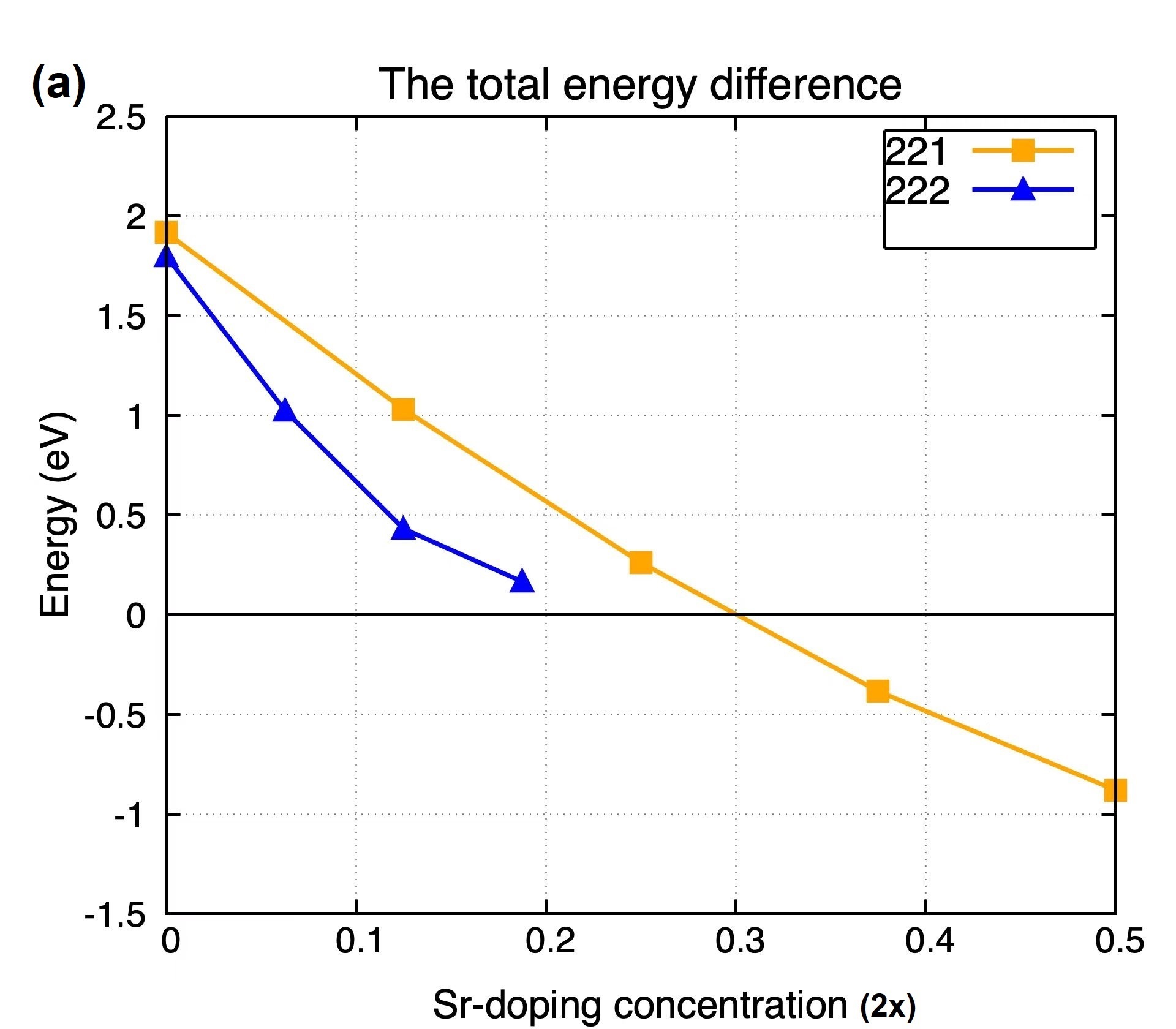
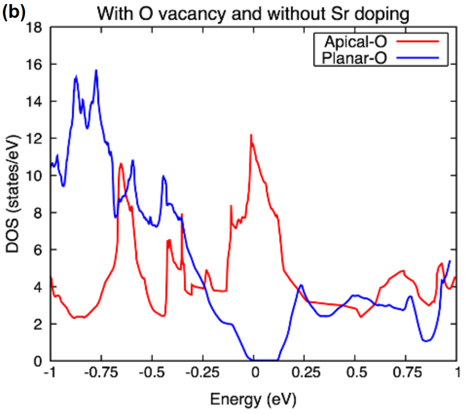
In order to determine the position of the oxygen vacancies theoretically, we performed first principle calculations on La2-xSrxCuO4-y within the local density approximation (LDA), which has been found to work very well in the overdoped cuprates Kramer et al. (2019). By constructing two kinds of super unit cells, and , with one oxygen vacancy, and optimizing the positions of the doped Sr atoms, we obtain the total energy difference between two kinds of oxygen vacancies as shown in Fig. 9(a). Without Sr doping, the planar oxygen vacancy is lower than the apical one , but upon Sr doping, their difference reduces and finally reverses at high doping levels. Such a tendency becomes stronger when we enlarge the super unit cell from to , indicating the oxygen vacancies in overdoped LSCO are very likely to be apical rather than planar ones, in agreement with the Raman experiment Kim et al. (2017). This behavior can be roughly understood from the density of states (DOS), as shown in Fig. 9(b). As can be seen, the planner oxygen vacancy reduces the DOS near the Fermi level at and thus saves more energy. Instead, the apical vacancy enhances the DOS near the Fermi level. Upon hole doping caused by Sr, the DOS of the apical case is reduced and thus finally becomes preferred than the planar case.
III.2 Planar oxygen vacancies
From both the experiment and our LDA calculations, we have found the oxygen vacancies are dominated by apical ones in overdoped LSCO. However, at small doping, the planar ones are more stable. Therefore, we may also ask what happens for the planar oxygen vacancies?
At first, one planar oxygen vacancy breaks the Zhang-Rice singlets on its two neighboring sites. To describe such an effect, we consider a model by adding two onsite potentials given by
| (28) |
where the subscript labels the position of the vacancy is on the -bond or -bond, hence, , and generate electrons on , and , respectively. We call this scattering process as type-I. Its amplitude is given by
| (29) |
Such a disorder scattering is difficult to treat exactly as it depends on the transferred momentum (but not and independently like the apical case) and breaks the rotational symmetry. Nevertheless, let us qualitatively consider its role on the d-wave superconducting properties. If we keep only the dominant scattering processes, they occur at (for -bond vacancies)and (for -bond vacancies). These scatterings preserve the pairing sign and are expected to be not pair-breaking, in some sense like the point disorder in s-wave superconductors. Therefore, the standard nonmagnetic disorder effects on the conventional dirty s-wave superconductors are expected: such disorders should have little effect on but reduce the superfluid density. Furthermore, these scatterings do not vanish for nodal quasiparticles, hence, the scattering rate is finite in this region (like ) which cannot explain the linear -dependence of the superfluid density.
On the other hand, one planar oxygen vacancy can also change the hopping on this bond (called type-II process), which can be described by the following Hamiltonian
| (30) |
The symbols are similar to the above. The amplitude of this scattering potential is
| (31) |
which is largest at (for -bond vacancies) and (for -bond vacancies). These scatterings are also not pair-breaking and thus are expected to be similar to the above type-I scatterings.
Put these two processes together, we conclude that the planar oxygen vacancies behave more like pair-preserving disorders in d-wave superconductors and cannot explain the superfluid density experiment.
III.3 Current vertex correction
Now let us examine the effect of the current vertex correction caused by the anisotropic disorder scattering. We label the bare current vertex by and the dressed vertex by . They are connected in a self-consistent way as shown in Fig. 10, where we have neglected all crossing diagrams which are at least of order and are expected to be more relevant to localization Lee and Ramakrishnan (1985). In fact, the resistivity in the overdoped LSCO becomes smaller and smaller upon doping, indicating the system are more and more itinerant than localization Božović et al. (2016).
From Fig. 10, we can write down the self-consistent equation
| (32) |
For a general scattering , the above equation can be solved to give rise to an additional factor in the so-called transport scattering rate which enters Abrikosov et al. (1963). But here, in our model, it becomes quite simple because the disorder scattering potential is already factorized such that the summation over can be completed exactly. Moreover, notice that is time reversal () odd, while is time reversal even, the integral over must be zero, which means . Therefore, in our disorder model, the current vertex correction totally vanishes, if the crossing diagrams can be safely neglected.