Anisotropic odd elasticity with Hamiltonian curl forces
Abstract
A host of elastic systems consisting of active components exhibit path-dependent elastic behaviors not found in classical elasticity, which is known as odd elasticity. Odd elasticity is characterized by antisymmetric (odd) elastic modulus tensor. Here, from the perspective of geometry, we construct the Hamiltonian formalism to show the origin of the antisymmetry of the elastic modulus that is intrinsically anisotropic. Furthermore, both non-conservative stress and the associated nonlinear constitutive relation naturally arise. This work also opens the promising possibility of exploring the physics of odd elasticity in dynamical regime by Hamiltonian formalism.
Keywords: odd elasticity, anisotropic mass, Hamiltonian formalism
1 Introduction
In classical elasticity, the input work to deform the elastic body depends only on its initial and final states. Such path-independence is characterized by the elastic potential that yields conservative stress [1, 2]. Recently, it has been reported that the work involved in deformations is dependent on the path in a class of elastic systems consisting of active components, such as in robotic metamaterials [3, 4]. A common feature in these active systems is that nonzero work could be extracted in a cycle of deformation. The dependence of the work on the deformation path could be attributed to an additional antisymmetric (odd) part in the elastic modulus tensor, which is known as odd elasticity [5, 6, 7]. The broken major symmetry of odd-elastic modulus leads to the non-conservative nature of the stress and a series of phenomena not found in classical elasticity, such as the modification of defect strains, interactions and motility [6, 8, 9], and the emergence of non-Hermitian skin effect [3] and chiral edge waves [10].
In the continuum description of odd elasticity, the odd-elastic modulus can be obtained by the coarse-graining procedure of the non-conservative forces between constituents in the elastic body [6, 8, 11]. Experimental realizations of non-conservative interparticle forces include fluid-mediated spinning particle [12, 13], gyroscopic lattices [14, 15], vortices in superfluids [16, 17] and skyrmions [18, 19]. In previous studies, the phenomenon of odd elasticity is attributed the active components of the system. Theoretically, an antisymmetric modulus is introduced to successfully describe the odd-elasticity behaviors at the continuum level. Specifically, a common approach to investigating odd elasticity begins with the dynamic equation and the constitutive relation [5, 6, 7], where an antisymmetric odd-elastic modulus is introduced as a parameter. However, the origin of the antisymmetry of the odd-elastic modulus in general has not yet been fully understood. Exploring this fundamental scientific question yields deeper insights into the nature of odd elasticity, and it also has strong connection to the design of odd elastic systems. One challenge is that due to the nonzero curl, the non-conservative stress involved in odd elasticity is not derivable from a scalar potential like in classical elasticity.
In this work, a field theory in Hamiltonian formalism is constructed to produce the antisymmetric elastic modulus tensor that is essential for a host of odd elastic behaviors. Specifically, a -dimensional continuum elastic body is modeled as a Riemannian manifold embedded in the -dimensional Euclidean space, and the Hamiltonian for the elastic body of finite strain is constructed. The key is introducing an anisotropic tensorial effective mass in the kinetic energy term, as inspired by the work on Hamiltonian curl forces [20, 21, 22]. The resulting antisymmetric elastic modulus tensor also simultaneously inherits the anisotropic nature of the mass tensor. Note that the inherent anisotropy is distinct from the odd elastic modulus generated through other mechanisms [6, 7]. The constitutive relation associated with the non-conservative stress is nonlinear in general, and the nonlinearity originates from the intrinsic geometry of the deformed elastic body. This work provides insights into the origin of the antisymmetry of the elastic modulus tensor in odd elasticity, and opens the promising possibility of exploring the dynamics of odd elasticity in the Hamiltonian framework.
2 Model and Method
2.1 Geometric viewpoint of elastic deformation
An elastic body in continuum limit is modeled as a -dimensional Riemannian manifold embedded in Euclidean space in the study of its interior elastic deformation. The strain state is characterized by the metric tensor defined on . For example, the strain-free elastic body prior to any deformation is described by a Riemannian manifold isometrically embedded in Euclidean space; the value of is specified by the pullback of the Euclidean metric [23, 24]. Note that in this work we employ the abstract index notation in Latin letters to represent a tensor; the tensor components are labeled by Greek letters.
In general, the deformation of the body leads to the variation of the element of length, and thus the metric of the manifold [25, 26]. Therefore, the elastic deformation of the body could be characterized by a diffeomorphism from some reference configuration to the deformed one: . Note that subscripts ‘’ are to indicate that is a covariant tensor field of order 2. The topology of is preserved in elastic deformation. To illustrate the mapping, we present some examples in figure 1. Under the deformations as described by the mappings (), any given point in the reference configuration, say , is mapped to . The original 2D elastic body of square shape is deformed to a rectangle (by mapping), to the patches on the sphere (by mapping) and on the cylinder (by mapping), respectively. In these three kinds of deformations, refers to the Euclidean metric, the spherical metric and the cylindrical metric, respectively.
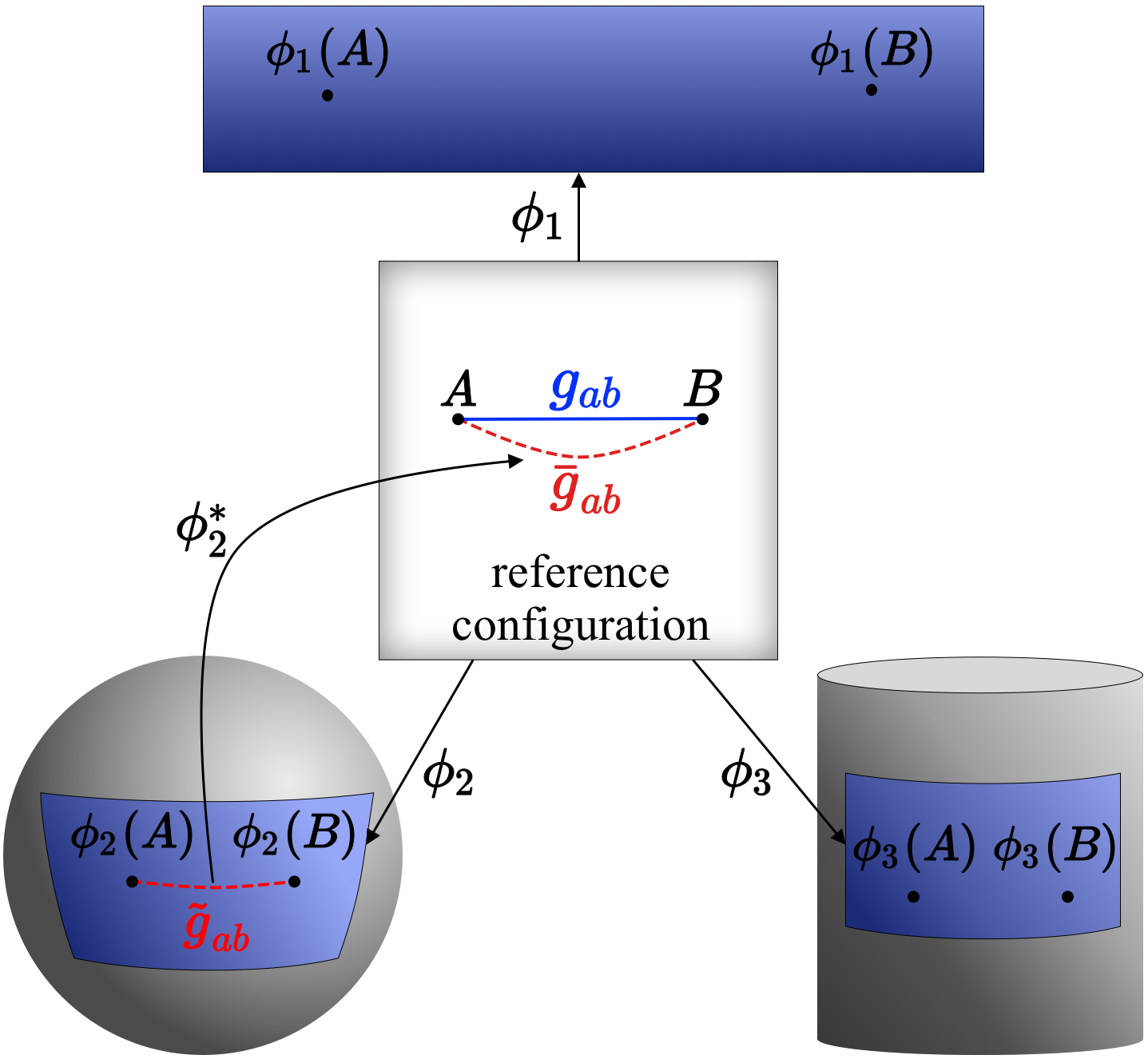
From the geometric perspective, the deformation is characterized by the variation of the metric from to , both of which are defined on the same manifold . Specifically, the information of the strain in the deformation is encoded in the difference between and . To illustrate this point, let us consider a curve , where . The length of the line element on is measured by . After the deformation, the curve is mapped to . The length of a line element on measured by is equal to the length of the corresponding line element on measured by . Therefore, the change of the curve length could be measured by . As such, it is natural to define the strain tensor on as [27, 2, 28]
| (1) |
where . The definition of strain in (1) is also applicable to large deformation [2].
In the following discussion, the Riemannian manifold is denoted as , representing the deformed configuration of the elastic body. The elastic body is initially free of stress, and is thus isometrically embedded in the -dimensional Euclidean space . The metric on the manifold is induced from the metric on [24, 29, 30], i.e., , where is the unit normal covector on in . For example, consider a 2D surface isometrically embedded in . One may construct the Cartesian coordinates centered at any point on the surface; -axis is perpendicular to the tangent plane at point . The first fundamental form (or the line element) is given explicitly by the metric: , where are local coordinates near the point . Note that the Greek letters in the indices represent the components of the tensor, and they take the values from to . Here, the convention of Einstein summation is applied. For spherical surface, and , where the polar angle and the azimuthal angle . Note that due to the isometric embedding of in , all of the tensors in this work are regarded as being defined on the tangent space of , and the lowering (or raising) of the indices of a tensor is uniformly implemented by (or ).
Now, we characterize the displacement field associated with the deformation in terms of the geometric language introduced in the preceding paragraph. We first establish the Cartesian coordinates system of by . The manifolds and are thus represented by the -valued functions and (), respectively. . The displacement field on is
| (2) |
where the -component of the displacement field
2.2 Construct Hamiltonian of the elastic body
The displacement fields constitute an infinite dimensional manifold called the configuration space. The Hamiltonian of the elastic body is a scalar on the cotangent bundle of the configuration space, and it can be written formally as [30]:
| (3) |
where and are the kinetic energy and elastic potential per unit mass, respectively. is the Riemannian volume form compatible with . is the mass density of the deformed configuration. In this work, is a quadratic local function of . The gradient of is recognized as the Kirchhoff stress tensor:
| (4) |
is a symmetric tensor field on . It measures the stress experienced by the unit mass of the deformed configuration. Note that the Cauchy stress tensor is related to the Kirchhoff stress tensor by , and it measures the stress on the unit volume of the deformed configuration [30]. In (3), could be written as a quadratic function of the generalized momentum density field that is conjugated to :
| (5) |
It is important to point out that here we introduce the effective mass tensor . is anisotropic and symmetric, and it is invariant in the deformation of the elastic body. In connection to possible experimental realizations, the anisotropy of may be introduced by designing a local resonance cavity structure composed of an internal mass that is connected to the wall by two perpendicular Hookean springs; such anisotropic mechanical microstructures have been used to regulate the propagation of acoustic waves in metamaterials [31, 32]. An explanatory example based on the modified mass-in-mass model is presented in section 3.4 to show the realization of anisotropic effective mass units. The idea of introducing the anisotropy in the construction of the kinetic energy is inspired by the work on Hamiltonian curl forces [20, 21, 22]. The concept of inducing Hamiltonian curl forces through anisotropic mass was initially introduced in systems with finite degrees of freedom by Berry and Shukla [20, 21, 22]. Specifically, it has been proved that a class of non-conservative (i.e., whose curl is not zero) position depending forces can be generated by the element of anisotropy in the kinetic energy term in Hamiltonian. Here, we extend this idea to the continuum elastic system by incorporating the non-conservative nature into . Consequently, (3) admits a non-conservative force density, which is crucial for understanding odd elasticity.
3 RESULTS AND DISCUSSION
3.1 Hamilton’s Equations
The Hamilton’s equations based on (3) are
| (6a) | |||
| (6b) | |||
where . Note that the repeated indices in pairs represents tensor contraction. is the determinant of ; is the Cartesian derivative operator on acting on the embedding coordinates of . The detailed information is presented in A and B. Note that the generalized coordinates in the Hamiltonian formalism is closely related to the strain of an elastic body.
By combining (6a) and (6b), we obtain the dynamic equation of the manifold as
| (6g) |
where the displacement velocity field and the symmetric tensor field . According to (6g), regulates the acceleration of unit mass in the elastic body, and it is recognized as the Newtonian force per unit mass. (6g) suggests that the dynamics of a continuum elastic body with anisotropic mass under is equivalent to the dynamics of a unit scalar mass under ; the velocity as associated to the displacement field is the common dynamics variable.
3.2 Hamiltonian curl forces and odd elasticity
Without any loss of generality, is decomposed as
| (6h) |
where , and is a traceless symmetric tensor field. Here, we shall emphasize that the anisotropic effect in the kinetic energy is captured by . By (6h), the kinetic energy density is divided into the isotropic and the anisotropic parts:
| (6i) |
We also cast in the following form
| (6j) |
Now, let us focus on (6j). The first term in (6j) is recognized as the force per unit mass as a derivative of the elastic potential for [28, 33, 34, 35]. According to (6a) and (6b), the power of is expressed as:
| (6k) |
In the last equality, the conservation of the total energy is applied, i.e., . According to (6k), the power of is equal to the reduction rate of . Due to the conservation of the total energy, it indicates that the work done by is equal to the energy transfer from the potential energy to the kinetic energy per unit mass in the deformation of the elastic body. Note that for a single-valued function, the integration of (6k) over any closed orbits in is zero, implying that is a conservative force. As such, the first term of in (6j) does not alter the value of either or in a cyclic deformation of the elastic body.
We proceed to examine the second term in (6j). The power of is:
| (6l) | |||||
Under the assumption that the anisotropic tensor is small compared with , (6l) becomes
| (6m) |
Here, it is important to point out that the R.H.S. of (6m) is identified as the rate of the increase of the anisotropic part of . In other words, the work done by causes the increase in the anisotropic part of the kinetic energy per unit mass.
In the following, we will show that the second term in (6j) is a non-conservative force. To this end, we first substitute the expression of in (6j), and obtain the expression for the Newtonian force per unit volume as
| (6n) | |||||
where . Note that is not symmetric. Furthermore, does not live in the tangent space of because of the acting of . For spatially-slowly-varying , its gradient could be regarded as a small quantity. Therefore, the last term in (6n) is much smaller than the second term; note that . As such, the last term could be neglected. The anisotropic effect boils down to the modification of in as shown in the first bracket in (6n).
Now, to reveal the non-conservative nature of the second term in (6j), we analyze the work done by the total stress per unit mass in a cyclic deformation. In the deformation process, the instantaneous strain state of the elastic body is denoted by , which is represented by a point in the space of the strain field . The cycle of deformation is thus described by a loop in the strain space. . . The work done per unit mass in a cycle of deformation is [6, 10]:
| (6o) | |||||
where , and is the surface enclosed by . Stokes’s theorem is used in the derivation for (6o). Since the exterior product is antisymmetric, the stress is conservative (such that in the cyclic deformation) if and only if possesses the major index symmetry, i.e., . Especially, quasi-static cyclic deformation can be realized by applying suitable external force on . is then equal to the work done by the external force.
We analyze the first term of in (6o). From the expression for
| (6p) |
where is the elastic modulus tensor with major index symmetry (i.e, ), we obtain the linear constitutive relation
| (6q) |
Due to the major index symmetry of , the first term of satisfies , which indicates the conservative nature of . In other words, the work done by is zero in a cyclic deformation.
For the second term in , from the definition of and (6q), we have
| (6r) | |||||
where
| (6s) |
In the nonlinear constitutive relation in (6r), the quadratic term naturally arises in the expansion of as the sum of the metric of the reference configuration and the strain field . Furthermore, the anisotropic tensor leads to the anisotropic nature of the elastic modulus and . Here, we shall point out that in the Hamiltonian formalism based on anisotropic mass tensor, the resulting odd elastic modulus are naturally anisotropic. The anisotropy of and is inherent in our formalism. A detailed discussion about the symmetry of and is in D. In general, the odd elastic modulus are not necessarily anisotropic in 2D [6]. By (6r), the second term of is obtained
| (6t) |
The bracket in the superscript of indicates the symmetric part of the tensor. Here, it is important to point out that in (6s), the involvement of the -tensor breaks the major index symmetry of , as well as that of the second and the third terms in the right hand side of (6t). Consequently, is non-conservative according to (6t).
Note that both and in (6s) are invariant in the deformation of . The reason is as follows. In the expressions for and , both the elastic modulus tensor and the metric are independent of the deformation of . Regarding the factor , according to (6h) and the definition for , , where is the mass density of the reference configuration. is therefore invariant in the deformation of .
In the regime of small deformation, where the quadratic term in (6r) can be neglected, the constitutive relation of becomes linear:
| (6u) |
The broken major index symmetry of indicates the presence of the
antisymmetric (odd) part in the elastic modulus tensor, which is responsible for
the non-conservativity of the stress and the extra work occurring in cyclic
deformations. As such, is called the odd elastic modulus in
literature [6]. Microscopic mechanism for odd elasticity has
been attributed to various non-conservative interparticle forces. Here, the odd
elasticity as characterized by the -tensor in
(6u) is derived from the anisotropic effective mass in the
Hamiltonian formalism in the continuum level.
We shall point out that in the model of odd elasticity based on the Hamiltonian formalism, the total energy is conserved. The work extracted by during cyclic deformations is from the conversion of the kinetic energy pre-stored in the internal degree of freedom of the system, rather than from the external energy inputs (see section 3.4 for detailed discussions). The anisotropy of the effective mass arises from the coarse-grained internal degrees of freedom. In a cyclic process, according to (6m), the non-conservative curl force transfers the kinetic energy between the (coarse-grained) anisotropic parts of and the isotropic parts of . As such, for a cyclic deformation starting and ending at zero velocity, no work can be extracted.
3.3 Example of 2D planar deformation
In this section, we illustrate the emergence of odd elasticity for the simple case of planar deformation of a 2D elastic body under small deformation approximation.
The strain tensor in the deformation can be expanded as , where is a set of orthogonal tensor bases on the reference configuration equipped with a local orthonormal frame fields [6]:
| (6va) | |||
| (6vb) | |||
| (6vc) | |||
| (6vd) | |||
characterizes the following local modes of deformation: dilation, rotation, and shearing. The stress tensor can also be expanded as , where are associated with pressure, torque density and shear stress.
The rotationally symmetric elastic modulus tensor field could be written as (see C for details):
| (6vw) |
where and are Lamé coefficients. In the tensor bases of , , and . From (6vw), we obtain
| (6vx) |
Correspondingly, (6q) is expressed as . and characterize the isotropic stretching rigidity and the isotropic shear rigidity, respectively. Note that the matrix in 6vx is invariant under the rotation of .
We proceed to discuss the components . By expanding the traceless tensor in the tensor bases of as
| (6vy) |
where and are scalars, we finally have
| (6vz) |
Since , the abstract index exchange in is identical to the label exchange in . (6vz) shows that , and therefore . This key feature of the broken major symmetry is exactly the mathematical structure underlying the phenomenon of odd elasticity. The upper right submatrix in (6vz) connects shear strain with pressure and torque, and the lower left submatrix connects dilation with shear stress. The existence of these two non-zero submatrices is an indicator for the anisotropy of [6].
3.4 Example of an anisotropic mass model
In the following, we employ the modified mass-in-mass model as an example to show the emergence of the anisotropic inertial mass and the non-conservative force.
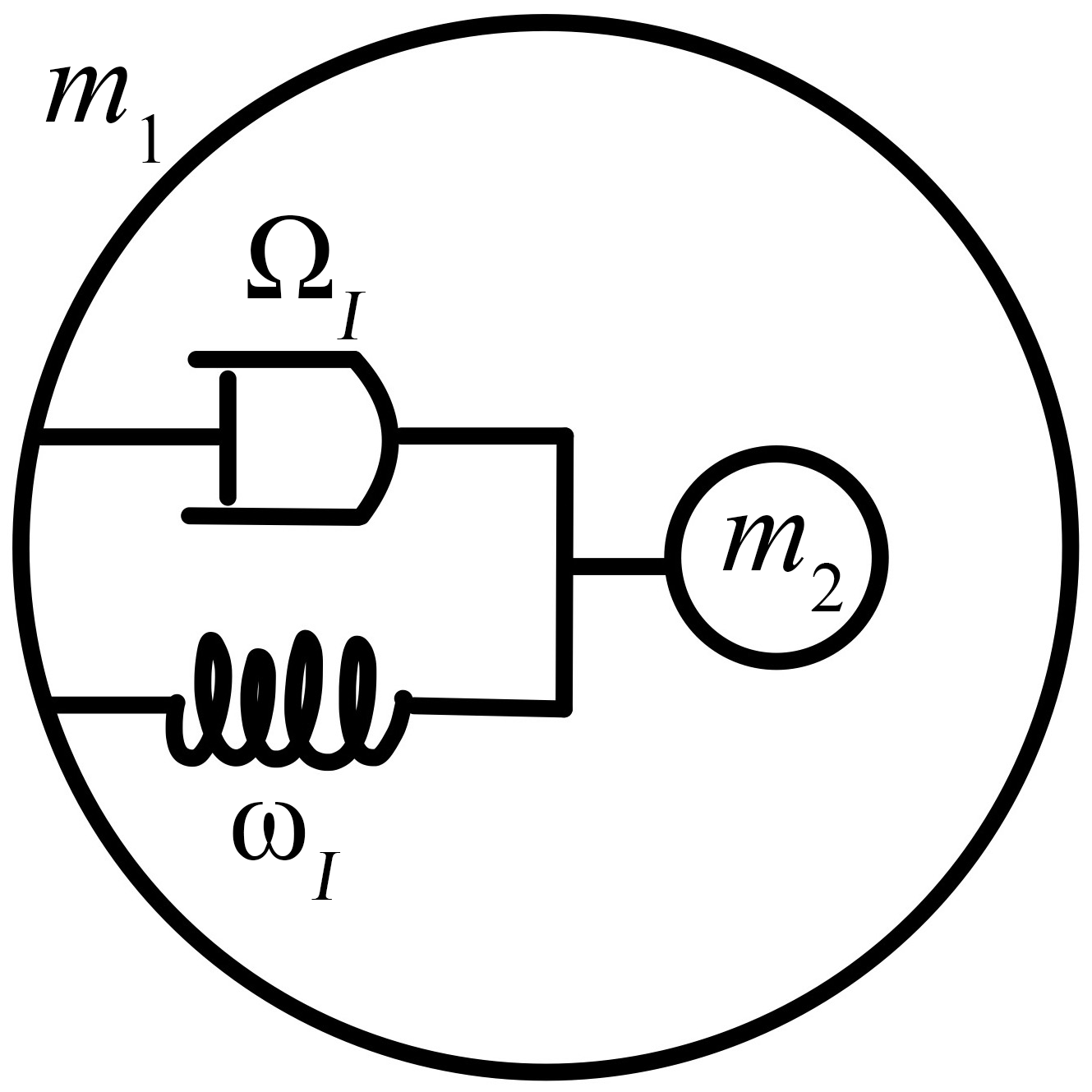
Consider a 2D cavity of mass that contains an internal mass , as illustrated in figure 2. The internal mass is connected to the cavity via a spring of resonance frequency and a damper of damping constant . The cavity is subject to an external potential . The dynamic equations for this mass-in-mass model are
| (6vaaa) | |||
| (6vaab) | |||
| (6vaac) | |||
| (6vaad) | |||
where and represent the Cartesian coordinates of displacements of and respectively, and .
We focus on the motion along the x-direction. Adding and subtracting (6vaaa) and (6vaab) lead to:
| (6vaaaba) | |||
| (6vaaabb) | |||
where the external force:
| (6vaaabac) |
and the dimensionless quantities are
| (6vaaabad) |
We focus on the regime of and , i.e., the dynamics of the internal degree of freedom is much faster than the that of the cavity.
We first analyze (6vaaabb) by introducing the following Green’s function :
| (6vaaabae) | |||||
where
| (6vaaabaf) |
We thus have:
| (6vaaabag) |
The integration over in (6vaaabag) is implemented by the residue theorem. Specifically,
| (6vaaabah) |
The integrand has two poles in the lower half complex -plane at:
| (6vaaabai) |
if .
By the standard method of constructing a closed contour via introducing an infinitely large semicircle in the lower half-plane, and applying the residue theorem, the first term in (6vaaabah) becomes
| (6vaaabaj) | |||||
By inserting (6vaaabah) and (6vaaabaj) into (6vaaabag), we obtain:
| (6vaaabak) | |||||
Note that the initial value theorem of Laplace transform is used in the integration over . The theorem states that for large real ,
| (6vaaabal) |
Consequently, (6vaaaba) is simplified to:
| (6vaaabam) |
Along with (6vaac), the equations of motion for the displacement are finally reduced to:
| (6vaaaban) |
where . Here, it is important to point out that the effective anisotropic mass arises in the mass-in-mass model. In Cartesian coordinates,
| (6vaaabao) |
Therefore, elastic media fabricated by connecting such cavity units with Hookean springs could manifest anisotropic mass density, and thus exhibit odd elasticity.
We proceed to discuss the Hamiltonian non-conservative force acting on the cavity. First of all, we construct the Hamiltonian corresponding to (6vaaaban) as
| (6vaaabap) |
The total kinetic energy includes the kinetic energies of and :
| (6vaaabaq) |
where , , . The Hamilton’s equations are:
| (6vaaabara) | |||||
| (6vaaabarb) | |||||
Combining (6vaaabara) and (6vaaabarb), the dynamics equation becomes:
| (6vaaabaras) |
where the effective scalar mass . Note that (6vaaabaras) could also be derived by multiplying at both side of (6vaaaban). (6vaaabaras) shows the dynamics of an anisotropic mass under the potential , which is equivalent to the dynamics of an isotropic mass subject to a non-conservative force .
By decomposing as
| (6vaaabarat) |
the total force is divided into the conservative part and the non-conservative part :
| (6vaaabarau) | |||||
One may check that in general the curl of is nonzero:
| (6vaaabarav) | |||||
Now, we analysis the work done by . Following the discussion in the main text, the total kinetic energy could be separated into the isotropic part and the anisotropic part as:
| (6vaaabaraw) | |||||
In a cyclic motion of along a closed orbit, the work done by the conservative force is equal to the change in the total kinetic energy, denoted as . Due to the energy conservation, . Therefore, is equal to . According to (6vaaabaraw), we obtain the following relations:
| (6vaaabarax) |
Consequently,
| (6vaaabaray) |
(6vaaabaray) reveals that in the cyclic motion of , the net work extracted by the non-conservative force , which is , is originated from the reduction of the kinetic energy of only.
4 Conclusions
In summary, from the perspective of geometry, we model a -dimensional continuum elastic body as a Riemannian manifold embedded in the -dimensional Euclidean space, and construct a Hamiltonian framework for the elastic body of finite strain. It is shown that the antisymmetry of the elastic modulus tensor is originated from the anisotropic mass tensor in the kinetic term. The resulting odd elastic modulus exhibits inherent anisotropy. We also derive the non-conservative stress and the associated nonlinear constitutive relation, where the nonlinearity is caused by the intrinsic geometry of the deformed elastic body. The Hamiltonian formalism constructed in this work for characterizing odd elasticity also allows one to explore the physics of odd elasticity in dynamical regime. We shall finally point out that our findings also raise some questions to be explored: Can the two features of antisymmetry and anisotropy of the elastic modulus be separated? Are there any other mechanisms to generate the characteristic antisymmetry of the odd-elastic modulus in the frame of Hamiltonian formalism?
Appendix A Expressions for the induced metric and strain
In this section, we derive the expressions for the induced metric and strain. Note that we employ the abstract index notation in Latin letters to represent a tensor; the tensor components are labeled by Greek letters. Abstract indices indicate the type of a tensor, with repeated indices in pairs denoting tensor contraction. The convention of Einstein summation is applied to repeated Greek indices.
First of all, for any local coordinates system on , the associated coordinates base vector on its embedding
| (6vaaabaraz) |
where is the Cartesian coordinates of the embedding of deformed configuration in the Euclidean space .
The isometric embedding of in the Euclidean space indicates that
| (6vaaabarba) |
where is the unit normal covector on . Therefore, the component of the metric tensor is
| (6vaaabarbb) | |||||
Here is the Euclid metric of , and is Kronecker delta which is the components of in Cartesian coordinates. In the derivation of (6vaaabarbb), we use the fact that . One has the similar result for as
| (6vaaabarbc) |
where is the Cartesian coordinates of the embedding of reference configuration.
By substituting (6vaaabarbb) and (6vaaabarbc) into the following expression of
| (6vaaabarbd) |
we obtain
| (6vaaabarbe) | |||||
where is the covariant derivative operator on . is metric compatible, i.e., . (6vaaabarbe) shows that could be regarded as a local function of .
Appendix B Variational derivatives of the Hamiltonian
In this section, we present the variational derivatives of the Hamiltonian defined on the manifold , which is recorded here
| (6vaaabarbf) | |||||
The variational derivative of the Hamiltonian with respect to the generalized momentum density field is
| (6vaaabarbg) |
To obtain the variational derivative of the Hamiltonian with respect to , we first calculate
| (6vaaabarbh) | |||||
Note that from the first line to the second line in (6vaaabarbh), the domain of integration is changed from the reference configuration to . In the last equality, we drop the divergence term to the boundary term by utilizing Gauss’s theorem; only the energy variation in the interior of the body is considered.
Now, we calculate the variational derivative of the Hamiltonian with respect to the displacement field :
| (6vaaabarbi) | |||||
is the derivative operator in the Cartesian coordinates on ; . is the exterior derivative operator on . is a projection operator: .
Here, it is of interest to point out that in general is not tangent to , which is shown below
| (6vaaabarbj) | |||||
where is the extrinsic curvature of . In the derivation, we use the definition of extrinsic curvature and the fact that . The first and second terms in (6vaaabarbj) are the tangent and normal components of [33, 34, 35]. For example, in the case of in figure 1 of the main text, the normal force supporting on the sphere is , where is the radius of the sphere and is the unit normal vector perpendicular to the spherical surface.
Appendix C The isometric symmetry of elastic modulus tensor
In the main text, we present the following expression for the rotationally symmetric elastic modulus tensor in an axisymmetric continuum elastic body:
| (6vaaabarbk) |
where and are Lamé coefficients. In this section, we present the derivation for (6vaaabarbk).
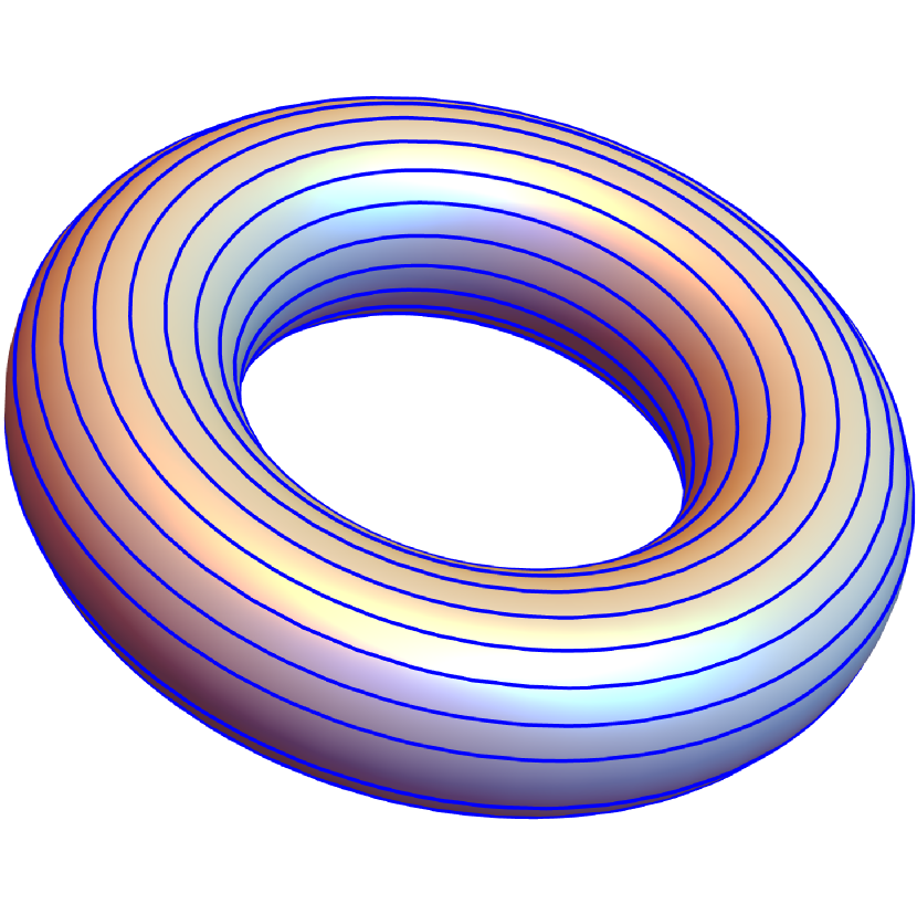
Consider an axisymmetric continuum elastic body. Its rotation as a whole belongs to a special isometric mapping that could be generated by a Killing vector field . By the definition of the Killing vector field, the displacement of the points from to leaves the distance relationships unchanged. In other words, the displacement of defines an isometric mapping. In figure 3(a), we present a 2D torus as an example of the axisymmetric elastic body. The tangent vectors of the toroidal lines constitute the Killing vector field on the torus. The elastic modulus tensor as associated with infinitesimal volume element possesses the rotational symmetry in the sense that it is invariant along the toroidal lines.
The rotational symmetry of the elastic modulus tensor is expressed by the zero Lie derivative of along the direction as specified by the Killing vector on the reference configuration [36]:
| (6vaaabarbl) | |||||
where is a Killing vector field satisfying , and is the covariant derivative operator on the reference configuration. as constructed by the tensor product of -tensors satisfies (6vaaabarbl); note that . Specifically, there are three kinds of index permutations of the tensor product:
| (6vaaabarbm) |
where , and are constant scalars on .
Due to the extra requirements for the conservation of angular momentum and the conservative nature of stress [6],
| (6vaaabarbn) |
The first equality is automatically satisfied for (6vaaabarbm). The second equality is satisfied if . The final expression for that satisfies both (6vaaabarbm) and (6vaaabarbn) is
| (6vaaabarbo) |
For Euclidean reference configuration, the components of in Cartesian coordinates system are
| (6vaaabarbp) |
By making use of the linear constitutive relation, the elastic potential can be expressed as
| (6vaaabarbq) |
where is the volume element of Cartesian coordinates on the reference configuration. In comparison with the linear elasticity theory, the parameters and are recognized as the Lamé coefficients [2].
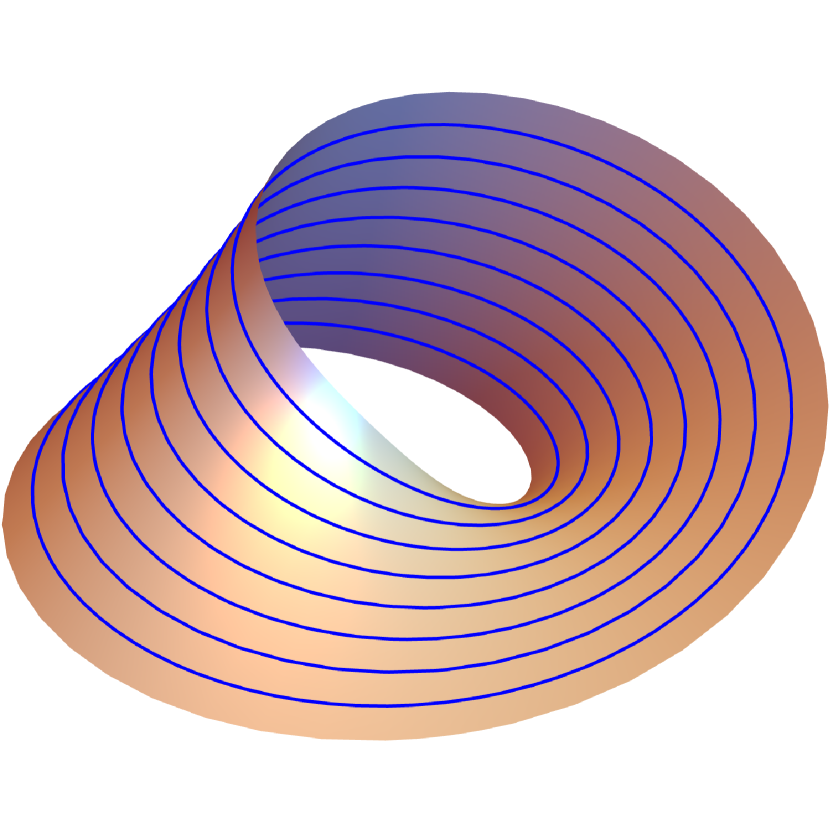
Note that (6vaaabarbl) could be used to describe the general case that the elastic modulus tensor is invariant along the lines of the Killing vectors, i.e., the isometric symmetry of the elastic modulus tensor. For example, on the Möbius strip in figure (3(b)), the tangent vectors of the lines constitute the Killing vector field; the isometric mapping of the Möbius strip is generated by this Killing vector field. that satisfies (6vaaabarbl) is invariant along these lines. This is the generalization of the rotational symmetry of the elastic modulus tensor of axisymmetric continuum elastic body as discussed in this section.
Appendix D The symmetry of and
In the main text, we assert that the odd elastic modulus and possess inherent anisotropy, which is different from traditional odd elastic modulus. Following the discussion in C about the symmetry of elastic modulus tensor, we can now further supplement the symmetry of and in details.
According to the definition in C, the sufficient and necessary condition for odd elastic modulus to be isometric is satisfied if and . Specifically, this requires to satisfy the following equation:
| (6vaaabarbr) |
where the isometric symmetry of is satisfied; and:
| (6vaaabarbs) |
where the isometric symmetry of is satisfied. Substituting (6vaaabarbs) into (6vaaabarbr) and eliminating the Lie derivative of , we obtain an identity. Therefore, (6vaaabarbr) and (6vaaabarbs) are equivalent, meaning the symmetries of and are consistent. In the following, we perform a detailed calculation of the symmetry of . The final result shows that, due to the coupling with , is necessarily anisotropic.
Generally, solving for Killing vector fields on a manifold is challenging. However, for simple cases, the corresponding Killing vector fields can be directly written using known properties of manifold symmetries, and the isometric condition for odd elastic modulus can be derived using (6vaaabarbl) or (6vaaabarbr).
First, let’s consider the case where the reference configuration is a 2D Euclidean plane ().
The 2D Euclidean plane has 3 independent symmetries: translations along the and axes, and rotation about the origin. The corresponding 3 Killing vector fields are: , , , where is the polar angle. Below, we denote the Lie derivative operators along these three Killing vector fields as , , . In this context, the translational and rotational symmetry of the 2D Euclidean plane correspond to the homogeneous and isotropy of the elastic modulus, respectively.
The analysis is divided into two steps: first, to determine the general form of the odd elastic modulus that satisfies the homogeneous isotropic condition, and then to find the that makes satisfy this condition.
We begin with (6vaaabarbl) to give the homogeneous isotropic condition for , that is, . In Cartesian coordinates, can be expanded as:
| (6vaaabarbt) |
If and only if are position-independent constant components, the following equations hold:
| (6vaaabarbu) | |||
| (6vaaabarbv) |
In this case, automatically satisfies the translational symmetry (homogeneous), and only the rotational symmetry (isotropy) condition needs to be considered. This condition is equivalent to the polar coordinate components of being independent of .
In the following, we derive for the rotational symmetry condition of in 2D.
The polar coordinate components of are obtained as follows:
| (6vaaabarbw) | |||||
where the Jacobian matrix transforms Euclidean coordinates to polar coordinates. The sufficient and necessary condition for to have rotational symmetry is:
| (6vaaabarbx) |
In deriving the above equation, we use the condition that , and thus , is a constant matrix. Solving this matrix equation for , we get:
| (6vaaabarby) |
with all other components being zero. When expressed in matrix form, it becomes:
| (6vaaabarbz) |
(6vaaabarbz) represents the isotropic condition for , with 6 independent stiffness coefficients, consistent with the results in the literature [6].
Next, we construct that makes satisfying (6vaaabarbz).
Since , we have:
| (6vaaabarca) |
Let be expanded in the frame as:
| (6vaaabarcb) |
where has the index symmetry, i.e., . Substituting (6vd), (6vy) and( 6vaaabarcb) into (6vaaabarca), we obtain the following matrix equation for :
| (6vaaabarcc) |
The condition for the solution of (6vaaabarcc) is that is non-degenerate, and the upper-left submatrix of matrix is equal to the lower-right submatrix, namely:
| (6vaaabarcd) |
This represents a specific odd elastic modulus with only 2 independent stiffness coefficients. The solution to (6vaaabarcc) is then:
| (6vaaabarce) |
Thus, by constructing a on the elastic body that satisfies (6vaaabarce) (which is evidently an anisotropic elastic modulus), one can obtain the homogeneous isotropic odd elastic modulus given by (6vaaabarcd).
According to our assumption, the rotation of the elastic body does not change its intrinsic geometry, and thus does not induce stress. Therefore, will also satisfy , or . At this point, (6vaaabarcc) only has the trivial solution . This implies that for a reference configuration of a 2D Euclidean plane, the odd elastic modulus and must be anisotropic due to the coupling with . It is known that any sufficiently small neighborhood of a point on a Riemannian manifold can be considered as a Euclidean space of the same dimension. Therefore, for any case of a 2D elastic body reference configuration, the odd elastic modulus and are anisotropic tensor fields.
Finally, some additional remarks on the assumption of are warranted. This assumption is known as the “objectivity” of the elastic body [2, 6], predicated on the premise that the interaction forces between the microscopic units of the elastic body depend only on their relative distance and not on the orientation. When a substrate exists, this condition may no longer hold [8, 37]. Thus, a more accurate statement is that, for any 2D elastic body possessing objectivity, the odd elastic modulus and are anisotropic tensor fields.
Next, we apply the above discussion to the case where the reference configuration is a 3D Euclidean space ().
A 3D Euclidean space has 6 independent Killing vector fields, corresponding to translational symmetry along the , , and axes: , , ; and rotational symmetry around the , , and axes: , , . Assuming that the Cartesian components of are still constant matrices, the homogeneous is automatically satisfied, and only its isotropic properties, i.e., rotational symmetry, need to be considered. We will next calculate the Lie derivatives , , and corresponding to the rotational symmetry around the , , and axes for .
To facilitate the consideration of rotational symmetry around the , , and axes, three sets of cylindrical coordinates are introduced as follows:
| (6vaaabarci) |
The components of in the three sets of cylindrical coordinates, (), can be obtained as follows:
| (6vaaabarcj) |
where the Jacobian matrix transforms Euclidean coordinates to cylindrical coordinates. The necessary and sufficient condition for to be isotropic, i.e., , is:
| (6vaaabarck) |
By solving this matrix equation for the constant matrix , we get:
| (6vaaabarcl) |
with all other coefficients being zero. It can be seen that in 3D, the isotropic odd elastic modulus has 3 degrees of freedom, fewer than the 6 in 2D. This is understandable as the isotropic odd elastic modulus in higher dimensions have higher symmetry, leading to more constraints. In fact, such high symmetry automatically imposes principal axis index symmetry on : from (6vaaabarcl), it is evident that . Therefore, 3D odd elastic modulus must be anisotropic. This is a consequence of fundamental symmetry, independent of the specific physical origin of the elastic modulus. This result is consistent with the conclusions drawn using group representation theory in the literature [6].
Similar to the 2D case, since any sufficiently small neighborhood of a point
on a 3D manifold can be considered as a 3D Euclidean space, for any 3D
elastic body reference configuration, the odd elastic modulus
and are anisotropic tensor fields.
Furthermore, from a physical standpoint, elastic bodies in dimensions higher
than 3 are generally not of interest. Therefore, we assert in the main text
that due to the contribution of the anisotropic mass ,
and naturally exhibit anisotropy.
References
- [1] Truesdell C A 1952 Indiana Univ. Math. J. 1 125–300 URL http://www.jstor.org/stable/24900260
- [2] Landau L D and Lifshitz E M 1960 Theory of Elasticity (Oxford: Pergamon)
- [3] Chen Y, Li X, Scheibner C, Vitelli V and Huang G 2021 Nat. Commun. 12 5935 ISSN 2041-1723 URL https://doi.org/10.1038/s41467-021-26034-z
- [4] Brandenbourger M, Scheibner C, Veenstra J, Vitelli V and Coulais C 2021 arXiv:2108.08837 URL https://arxiv.org/abs/2108.08837
- [5] Salbreux G and Jülicher F 2017 Phys. Rev. E 96(3) 032404 URL https://link.aps.org/doi/10.1103/PhysRevE.96.032404
- [6] Scheibner C, Souslov A, Banerjee D, Surówka P, Irvine W T M and Vitelli V 2020 Nat. Phys. 16 475–480 ISSN 1745-2481 URL https://doi.org/10.1038/s41567-020-0795-y
- [7] Fruchart M, Scheibner C and Vitelli V 2023 Annu. Rev. Condens. Matter Phys. 14 471–510 ISSN 1947-5454 URL https://doi.org/10.1146/annurev-conmatphys-040821-125506
- [8] Braverman L, Scheibner C, VanSaders B and Vitelli V 2021 Phys. Rev. Lett. 127(26) 268001 URL https://link.aps.org/doi/10.1103/PhysRevLett.127.268001
- [9] Bililign E S, Balboa Usabiaga F, Ganan Y A, Poncet A, Soni V, Magkiriadou S, Shelley M J, Bartolo D and Irvine W T M 2022 Nat. Phys. 18 212–218 ISSN 1745-2481 URL https://doi.org/10.1038/s41567-021-01429-3
- [10] Fossati M, Scheibner C, Fruchart M and Vitelli V 2022 arXiv:2210.03669 URL https://arxiv.org/abs/2210.03669
- [11] Poncet A and Bartolo D 2022 Phys. Rev. Lett. 128(4) 048002 URL https://link.aps.org/doi/10.1103/PhysRevLett.128.048002
- [12] Happel J and Brenner H 1983 Low Reynolds Number Hydrodynamics: with Special Applications to Particulate Media vol 1 (Springer)
- [13] Jäger S and Klapp S H L 2011 Soft Matter 7 6606–6616 ISSN 1744-683X URL https://doi.org/10.1039/C1SM05343D
- [14] Brun M, Jones I S and Movchan A B 2012 Proc. R. Soc. A. 468 3027–3046 URL https://royalsocietypublishing.org/doi/abs/10.1098/rspa.2012.0165
- [15] Nash L M, Kleckner D, Read A, Vitelli V, Turner A M and Irvine W T M 2015 Proc. Natl. Acad. Sci. U.S.A. 112 14495–14500 URL https://www.pnas.org/doi/abs/10.1073/pnas.1507413112
- [16] Tkachenko V K 1969 Sov. J. Exp. Theor. Phys. 29 945 URL http://www.jetp.ras.ru/cgi-bin/e/index/e/29/5/p945?a=list
- [17] Nguyen D X, Gromov A and Moroz S 2020 SciPost Phys. 9 076 URL https://scipost.org/10.21468/SciPostPhys.9.5.076
- [18] Ochoa H, Kim S K, Tchernyshyov O and Tserkovnyak Y 2017 Phys. Rev. B 96(2) 020410 URL https://link.aps.org/doi/10.1103/PhysRevB.96.020410
- [19] Benzoni C, Jeevanesan B and Moroz S 2021 Phys. Rev. B 104(2) 024435 URL https://link.aps.org/doi/10.1103/PhysRevB.104.024435
- [20] Berry M V and Shukla P 2012 J. Phys. A: Math. 45 305201 URL https://dx.doi.org/10.1088/1751-8113/45/30/305201
- [21] Berry M V and Shukla P 2013 J. Phys. A: Math. 46 422001 URL https://dx.doi.org/10.1088/1751-8113/46/42/422001
- [22] Berry M V and Shukla P 2015 Proc. R. Soc. A. 471 20150002 URL https://royalsocietypublishing.org/doi/abs/10.1098/rspa.2015.0002
- [23] Efrati E, Sharon E and Kupferman R 2009 J. Mech. Phys. Solids 57 762–775 ISSN 0022-5096 URL https://www.sciencedirect.com/science/article/pii/S0022509608002160
- [24] Kupferman R, Olami E and Segev R 2017 J. Elast. 128 61–84 ISSN 1573-2681 URL https://doi.org/10.1007/s10659-016-9617-y
- [25] Noll W 1978 A general framework for problems in the statics of finite elasticity Contemporary Developments in Continuum Mechanics and Partial Differential Equations (North-Holland Mathematics Studies vol 30) ed de la Penha G M and Medeiros L A J (North-Holland) pp 363–387 URL https://www.sciencedirect.com/science/article/pii/S0304020808708727
- [26] Rougée P 1992 The intrinsic lagrangian metric and stress variables Finite Inelastic Deformations — Theory and Applications ed Besdo D and Stein E (Berlin, Heidelberg: Springer) pp 217–226 ISBN 978-3-642-84833-9
- [27] Bilby B A, Bullough R, Smith E and Whittaker J M 1955 Proc. R. Soc. Lond. A 231 263–273 URL https://royalsocietypublishing.org/doi/abs/10.1098/rspa.1955.0171
- [28] Kochetov E A and Osipov V A 1999 J. Phys. A: Math. Gen. 32 1961–1972 URL https://doi.org/10.1088/0305-4470/32/10/013
- [29] Segev R and Epstein M (eds) 2020 Geometric Continuum Mechanics (Adv. Mech. Math. vol 43) (Cham: Birkhäuser) ISBN 978-3-030-42682-8; 978-3-030-42685-9; 978-3-030-42683-5
- [30] Kolev B and Desmorat R 2021 J. Elast. 146 29–63 ISSN 1573-2681 URL https://doi.org/10.1007/s10659-021-09853-5
- [31] Liu Z, Zhang X, Mao Y, Zhu Y Y, Yang Z, Chan C T and Sheng P 2000 Science 289 1734–1736 URL https://doi.org/10.1126/science.289.5485.1734
- [32] Huang H H and Sun C T 2011 Philos. Mag. 91 981–996 ISSN 1478-6435 URL https://doi.org/10.1080/14786435.2010.536174
- [33] Capovilla R and Guven J 2002 J. Phys. A: Math. Gen. 35 6233 URL https://dx.doi.org/10.1088/0305-4470/35/30/302
- [34] Capovilla R and Guven J 2004 J. Phys.: Condens. Matter 16 S2187 URL https://dx.doi.org/10.1088/0953-8984/16/22/018
- [35] Guven J 2004 J. Phys. A: Math. Gen. 37 L313 URL https://dx.doi.org/10.1088/0305-4470/37/28/L02
- [36] Lang S 2012 Fundamentals of Differential Geometry vol 191 (Springer Dordrecht)
- [37] Nelson D R and Halperin B I 1979 Phys. Rev. B 19(5) 2457–2484 URL https://link.aps.org/doi/10.1103/PhysRevB.19.2457