11email: [email protected] 22institutetext: Key Laboratory of Stars and Interstellar Medium, Xiangtan University, Xiangtan 411105, China 33institutetext: Department of Astronomy and Space Science, Chungnam National University, Daejeon, Republic of Korea
Anisotropic diffusion of high-energy cosmic rays in magnetohydrodynamic turbulence
Abstract
Context. The origin of cosmic rays (CRs) and how they propagate remain unclear. Studying the propagation of CRs in magnetohydrodynamic (MHD) turbulence can help to comprehend many open issues related to CR origin and the role of turbulent magnetic fields.
Aims. To comprehend the phenomenon of slow diffusion in the near-source region, we study the interactions of CRs with the ambient turbulent magnetic field to reveal their universal laws.
Methods. We numerically study the interactions of CRs with the ambient turbulent magnetic field, considering pulsar wind nebula as a general research case. Taking the magnetization parameter and turbulence spectral index as free parameters, together with radiative losses, we perform three group simulations to analyze the CR spectral, spatial distributions, and possible CR diffusion types.
Results. Our studies demonstrate that (1) CR energy density decays with both its effective radius and kinetic energy in the form of power-law distributions; (2) the morphology of the CR spatial distribution strongly depends on the properties of magnetic turbulence and the viewing angle; (3) CRs suffer a slow diffusion near the source and a fast/normal diffusion away from the source; (4) the existence of a power-law relationship between the averaged CR energy density and the magnetization parameter is independent of both CR energy and radiative losses; (5) radiative losses can suppress CR anisotropic diffusion and soften the power-law distribution of CR energy density.
Conclusions. The distribution law established between turbulent magnetic fields and CRs presents an intrinsic property, providing a convenient way to understand complex astrophysical processes related to turbulence cascades.
Key Words.:
galaxies: ISM – galaxies: magnetic fields – magnetohydrodynamics (MHD) – ISM: cosmic rays – ISM: diffusion1 Introduction
Cosmic rays (CRs) are charged particles moving with relativistic speeds, which can be directly detected in and near the solar system and indirectly observed from the emissions they produce far from the solar system (such as in the Milky Way and another galactic disk; Armillotta et al. 2022). Exploring the propagation processes of the Galactic CRs, including advection, diffusion, scattering, acceleration/reacceleration, and energy loss processes, will help to understand their origins (Castellina & Donato 2005; Strong et al. 2007; Blasi 2013; Grenier et al. 2015). Since propagating CRs will inevitably interact with turbulent magnetic fields, it also provides a useful tool for probing the properties of the interstellar medium (ISM).
Magnetohydrodynamic (MHD) turbulence is ubiquitous in astrophysical plasmas ranging from interplanetary space to interstellar and intergalactic media. It has been pointed out that MHD turbulence directly or indirectly affects the propagation of CRs. Studying the propagation of CRs in turbulent magnetic fields can help us to comprehend many important issues both in space and astrophysics, e.g., solar modulation of CRs (Jokipii & Parker 1969), driving Galactic winds (Wiener et al. 2017; Krumholz et al. 2020), CR anisotropy (Qiao et al. 2023; Li et al. 2024), X-rays binaries (Zhang et al. 2018), diffuse ray emission (Yan et al. 2012), as well as the confinement and reacceleration of CRs (Chandran 2000; Yan & Lazarian 2002; Zhang & Xiang 2021; Gao & Zhang 2024).
The High-Altitude Water Cherenkov Observatory (HAWC) collaboration first reported the TeV ray halos around the pulsars Geminga and Monogem (PSR B0656+14), with a spatial extension of 10-50 pc (Abeysekara et al. 2017). They explained these observations by the inverse Compton (IC) scattering process, that is, the high-energy CR electrons and positrons are injected from the pulsar wind nebula (PWN) and diffuse into the ISM to scatter off cosmic microwave background photons. Abeysekara et al. (2017) modeled the surface brightness profile of the ray emission of these two TeV halos to constrain a low diffusion coefficient of at 100 TeV. This diffusion coefficient is hundreds of times lower than the average value in the Milky Way as inferred from the secondary-to-primary ratio measurements in the CR spectrum (i.e., the boron-to-carbon ratio (B/C); Aguilar et al. 2016). This suggests that the diffusion coefficient may be highly inhomogeneous on a small scale. It could be meaningful to investigate the origin of this slow-diffusion region around the pulsars, which can help us to understand many important issues, such as the CR position excess (Hooper et al. 2017; Fang et al. 2018, 2019b; Tang & Piran 2019; Xi et al. 2019; Manconi et al. 2020), diffusion TeV ray excess (Linden & Buckman 2018; Yan et al. 2024), and particle propagation near CR source (Recchia et al. 2021; López-Coto et al. 2022).
At present, there are mainly three plausible explanations for this slow diffusion as follows. Firstly, this slow diffusion is explained by the projection effects under the framework of anisotropic diffusion, which requires the nearby turbulent environment to be sub-Alfvénic and a small viewing angle between the local mean magnetic field and the line of sight (LOS) (Liu et al. 2019; De La Torre Luque et al. 2022; Fang et al. 2023). Secondly, it may be caused by the turbulent environment generated by the parent supernova remnants of the pulsars (Fang et al. 2019a) or the escaped electrons themselves (Evoli et al. 2018; Mukhopadhyay & Linden 2022). Alternatively, the mirror diffusion111Lazarian & Xu (2021) found that in MHD turbulence CRs would not be trapped, due to the perpendicular super-diffusion of turbulent magnetic fields (Xu & Yan 2013; Lazarian & Yan 2014; Hu et al. 2022). On the contrary, they bounce between different magnetic mirrors and move along the local magnetic field, which leads to a new diffusion mechanism called mirror diffusion. With the stochastic change of pitch angles due to gyroresonant scattering, CRs undergo slow mirror diffusion at relatively large pitch angles and fast scattering diffusion at smaller pitch angles, resulting in a Levy-flight-like propagation that is slower than that induced by scattering alone (Xu 2021; Zhang & Xu 2023; Barreto-Mota et al. 2024; Xiao et al. 2024). As estimated in Barreto-Mota et al. (2024), the physical value of the diffusion coefficient is for 100 TeV CRs within an extended zone with tens of pc, which is consistent with the expected value to explain the observations of extended sources such as Geminga and Monogem (Abeysekara et al. 2017). may be a channel for understanding this slow diffusion process because the combination of resonance scattering with mirror diffusion can cause a slower diffusion than that induced by scattering alone (Lazarian & Xu 2021; Xu 2021; Zhang & Xu 2023; Barreto-Mota et al. 2024).
Due to the presence of ubiquitous magnetic turbulence, the resulting CR anisotropic diffusion may be reasonable in the key astrophysical environments (Holod et al. 2005; Parrish & Stone 2005; Parrish et al. 2008) and has obtained theoretical support (Evoli et al. 2012; Cerri et al. 2021). Recently, to explain the slow diffusion coefficient, the size, and morphology of observed TeV halos, Liu et al. (2019) and De La Torre Luque et al. (2022) limited the Alfvén Mach number to a small value of , and the viewing angle to . To some extent, these two small phase spaces may impede the application of the anisotropic diffusion model.
The main motivations for the current work are the need for slow diffusion to explain the observations mentioned above and for the narrow parameter space constraints in the anisotropic diffusion model. Therefore, in the framework of CR anisotropic diffusion, we explore the interactions of high-energy electrons with the ambient turbulent magnetic fields, considering PWN, i.e., the Crab-like nebula, as a general research case. We want to know whether the slow-diffusion phenomenon could happen in a reasonable parameter space. The relevant CR diffusion law related to MHD turbulence theory to what extent is applicable for understanding the transport of CR particles.
This paper is organized as follows. In Sect. 2, we briefly introduce the theoretical description of diffusion properties of CRs in MHD turbulence, including the energy-dependent parallel diffusion and anisotropic diffusion model. We perform a parameterized simulation and describe our initial simulation setup in Sect. 3. We present the numerical results in Sect. 4. Discussion and summary are provided in Sects. 5 and 6, respectively.
2 Theoretical basis
The propagation process of CRs can be described with the Fokker-Planck equation (Gaisser 1990; Berezinskii et al. 1990; Schlickeiser 2002), which is defined by
| (1) | ||||
where is the CR distribution function in the position space and the kinetic energy space . is the coordinate along the mean magnetic field, and is the coordinate perpendicular to the mean magnetic field. and are the spatial diffusion coefficients parallel to the mean magnetic field and perpendicular to it, respectively. is the energy diffusion coefficient (Michałek & Ostrowsky 1996), and is the rate of energy loss. In the case of power-law injection, the source function is defined by , where with a power-law index over the range from to . While for mono-energy injection, the source function is defined by , where , , and are the source luminosity, initial energy, and mass of the injected electrons, respectively.
2.1 The effect of the scaling properties of MHD turbulence on the spatial diffusion
It has been claimed that the propagation of CRs in the parallel direction with respect to the mean magnetic field is associated with the spectral properties of their ambient turbulent magnetic fields. In general, the parallel diffusion coefficient characterizing CR propagation can be described by the following empirical relation associated with the CR kinetic energy (Seo & Ptuskin 1994; Trotta et al. 2011; Dempers & Engelbrecht 2020)
| (2) |
where and are the light speed and diffusion index, respectively. The normalized spatial diffusion coefficient is set to be the typical ISM diffusion value, , throughout the work (Heesen et al. 2019). It was claimed that the diffusion index of [0.3, 0.6] could match CR observations in the Milky Way remarkably well (Strong et al. 2007; Trotta et al. 2011; Gaggero et al. 2014; Hopkins et al. 2022).
The spectral energy density of interstellar turbulence presents a power-law relationship of , where and are the wave number and turbulence spectral index, respectively. The power-law index (known as a Kolmogorov spectrum Kolmogorov (1941); i.e., 1/3) over a wide range of wave numbers (Elmegreen & Scalo 2004) determines the scaling law of the energy-dependent parallel diffusion coefficient . Theoretically, the Kolmogorov-type spectrum may refer only to a part of the MHD turbulence that includes the anisotropic (Alfvénic or slow modes) structures strongly elongated the mean magnetic field direction (Goldreich & Sridhar 1995, hereafter GS95; Cho & Lazarian 2002). On the other hand, there may exist another isotropic (fast mode) part of the turbulence in the ISM (Cho & Lazarian 2002), with the exponent (i.e., = 1/2) typical for the Kraichnan-type turbulence spectrum (Kraichnan 1965), in which the scaling of is close to the high-energy asymptotic form of the diffusion coefficient obtained in the plain diffusion version of the empirical propagation model. In addition, in the case of Bohm-type diffusion, the diffusion index is typically assumed to be 1 (Caballero-Lopez et al. 2004; Kempski & Quataert 2022; Lu et al. 2023).
2.2 The effect of the magnetization parameter on the spatial diffusion
The propagation of CRs is subject to their interactions with turbulent magnetic fields. As expected, the ratio of the perpendicular diffusion coefficient to the parallel component should depend on the magnetization parameter, i.e., the Alfvén Mach number , with the power-law relationship of
| (3) |
which is the so-called anisotropic diffusion model.
In the case of the sub-Alfvénic turbulence, corresponding to a strong magnetic field, i.e., the field that cannot be easily bent at the turbulence injection scale , individual magnetic field lines are aligned with the mean magnetic field. Note that Yan & Lazarian (2008) stressed the importance of dependence, in contrast to the dependence in the classical studies (Jokipii & Parker 1969; Kóta & Jokipii 2000). Later, analytical (Lazarian & Yan, 2014) and numerical (Xu & Yan, 2013; Maiti et al., 2022) results suggested a power-law index 4 in both scales that are larger and less than .
For the super-Alfvénic turbulence, Lazarian & Yan (2014) predicted a diffusion relation of the index 3 in the strong turbulence range of , where the and are the dissipation and transition scales, respectively. Namely, the dependence of from CR diffusion reflects the scenario that the GS95 cascade starts at rather than at the injection scale of turbulence . This point has obtained support from simulations (Maiti et al., 2022). However, in the weak turbulence range from to , it has been predicted as the power-law index 0 (Lazarian & Yan, 2014), which means the diffusion is isotropic. In other words, the perpendicular diffusion coefficient is the same as the parallel one, i.e., . This point still needs a numerical test.
3 Numerical setup
To explore the interactions of high-energy particles with ambient magnetic turbulence, we numerically solve Eq. (1) using the CR transport code CRIPTIC (Krumholz et al. 2022). With a PWN environment, we consider a uniform region containing gas with a density of and velocity of 300 , threaded by a uniform magnetic field in the -axis direction. For the general environment of PWN, we have the typical temperature of thermal gas of K (Zyuzin et al. 2021) and the sonic speed of 200 , resulting in a slightly supersonic Mach number of . When involving radiative loss processes, we consider synchrotron radiative losses of relativistic electrons due to the presence of the ISM magnetic field and IC scattering losses due to both interstellar radiation field with a temperature of 20 K and cosmic microwave one in the Klein-Nishina regime.
With the purpose of exploring how the magnetization parameter and turbulence spectral index affect particles’ diffusion behavior222In practice, we control the value of by regulating the turbulent magnetic field strength . For example, setting , one has . , together with various radiative processes, we divide our simulations into three groups:
-
•
: the influence of radiative losses on CR diffusion. In this case, with the fixed 5/3 and , we change the energy range and distribution of CR electrons. We consider two distribution types of CR electrons: a power-law energy distribution of with 2.2 over the range from to , and another mono-energy distribution.
-
•
: the influence of turbulence spectral index on CR diffusion. With the fixed and a series of mono-energy distributions, we change the spectral index of magnetic turbulence, corresponding to the different turbulence types.
-
•
: the influence of the magnetization parameter on CR diffusion. After fixing 5/3, we mainly consider the changes of the magnetization parameter , which will match with different magnetic field strength.
In the framework of the three groups described above, we run 90 sets of simulations up to with an output step of about 10 yr, considering the limited saving abilities of the data. Given a constant injection with the particles injection rate , the simulations include amounts of particles. For more details, the interested reader can refer to Appendix A for numerical procedures.
4 Numerical results
4.1 CR’s spectral distribution
As seen in Eq. (1), the CR distribution function is a function of the position , the kinetic energy , and the time . Therefore, what we first explore is the behavior of the CR distributions associated with its energy density in units of (see Krumholz et al. (2022) for analytical solutions of ), where the effective radius of particles is defined as , with the factor corresponding to the anisotropy level between the perpendicular diffusion and the parallel one.333The reason why we make the change of variables from to is simply for the purposes of changing the form of the equation to one for which a standard Green’s function solution exists. Consequently, the energy density would be a function of radius and not related to angle. It should be noted that the diffusion radius is , which should be distinguished from the effective radius .
4.1.1 Effect of radiative losses on CR distributions


In the energy range from 1 GeV to 10 PeV, the energy density as a function of the effective radius and the evolution time is shown in Fig. 1(a) in the absence of radiative loss, from which can see that the time-dependent evolution of the energy density with the effective radius presents a power-law relationship of near the source region and then cuts off exponentially. With time evolution, distributions almost follow the same power law with a gradually increasing range. After kyr (orange-red curves), vs. reaches a statistical steady state. The fluctuations that appeared at different times are a result of the deviation from statistics. This result may imply that the CR electrons are suffering from slow diffusion near the source and fast/normal diffusion away from the source, which will help to understand observations of slow diffusion around the pulsar (Abeysekara et al. 2017).
To explore CR distributions from different energy particles, we divide the whole energy band into individual energy regimes: the GeV ( GeV), TeV ( GeV), and PeV ( GeV) range, as well as a wide range from to GeV. Focusing on a comparison study with/without radiative loss processes, we provide the results in Fig. 1(b) obtained at the final snapshot. Without radiative losses, distributions at different energy ranges remain a relation of around the source (about several or multi-tens pc) and then it enters the exponential decay stage. After including radiative losses, we see that with increasing the kinetic energy, the effect of loss processes gradually becomes stronger. In particular, the radiative losses modify the particle distribution in the PeV range, presenting a steeper power-law of . In this regard, the maximum effective radius the particles can reach is smaller, and the spatially extended power law range is narrower.
Based on the same simulation setup used in Fig. 1(a), we plot in Fig. 1(c) the evolution of energy density over the kinetic energy of CR electrons at the different evolution times. As is seen from this panel, presents a power-law relationship of with an exponential high-energy cutoff. In addition, we also see a feature of the three discrete distributions of the energy density (rather than changing continuously): (1) the maximum energy of GeV at about 10 yr; (2) GeV from yr to yr, and (3) GeV at multi-thousand yr. The power law relation of we find is approximate to the initial injection form of , i.e., a power-law energy injection of with 2.2 in Group . Here, the slight hard power-law index feature should be a result of a weak stochastic acceleration process (associated with the third term of Eq. (1) on the right-hand side). As a result, the evolution processes of CR electrons result in a modification of the power-law distribution, in particular the occurrence of a significant exponential cutoff.
Similar to Fig. 1(b), we show the distribution of vs. the energy in Fig. 1(d) at the final snapshot. In the absence of radiative losses, the CR electrons have a spectral energy distribution of , the slightly hardened spectral index of which is due to a weak acceleration process as explained in Fig. 1(c). When involving loss processes, the energy density presents a steeper relation of with a significant exponential cutoff in the PeV range. This process gives rise to a change of compared with the scenario without losses. However, when compared with the initial distribution of , there is a change of . This indicates that the diffusion processes are dominated by a strong radiative loss, resulting in the potential PeV observations (e.g., Cao et al. 2021, 2024). Furthermore, the particle distribution with a power law plus an exponential cutoff is suggested when understanding high-energy observations.
4.1.2 Effect of MHD turbulence properties on CR distributions


Based on the final snapshot simulations from Group , we show the energy density as a function of the effective radius and the magnetization parameter in Fig. 2(a). As studied in Sect. 4.1.1, given that the effect of the loss processes is significant only in the high-energy regime, at least PeV-order of magnitude, we here just show the results of mono-energy injection at 1 PeV. The overall distribution of vs. in various remains similar to that of the power law injection, i.e., presenting a power-law transition from (without loss) to (with loss). With increasing the magnetization parameter , the value of decreases, where CR electrons will diffuse away from the source and up to a larger spatial scale. This is because the larger means a weaker magnetic field, i.e., weaker magnetic trapping effect, then the spatial extent caused by diffusion will be wider. Comparing the sub-Alfvénic () with super-Alfvénic turbulence regime (), they are similar from the perspective of the overall power-law distribution. When focusing on the case of radiative losses (solid curves), we find that the increment of the maximum effective radius pc for the sub-Alfvénic turbulence is smaller than that pc for the super-Alfvénic turbulence. This may be due to the different dependence of the perpendicular diffusion coefficient on , i.e., for the sub-Alfvénic regime, while for the super-Alfvénic case (see Sect. 2.2). This manifests that the magnetization parameter , is of great importance to the CR’s spectral distribution.
Fig. 2(b) shows the energy density as a function of the effective radius with various , based on the last simulation snapshot from Group . As shown, the power-law transition is similar to that of Fig. 2(a). With increasing the turbulence spectral index, the effective radius decreases while the energy density increases. We note that as decreases, the fluctuation of the spectral distribution increases within several pc scales, which may be due to the effects of insufficient statistical samples and strong radiative losses. This demonstrates that the scaling of MHD turbulence is an important factor in the CR’s spectral distribution.
4.2 CR’s anisotropy
4.2.1 Effect of radiative losses on CR anisotropy


We show the projected energy density at the final snapshot for the power-law distribution of Group in Fig. 3, including the non-loss case of GeV projected in three different planes (upper row), the non-loss case of three narrow energy ranges projected in plane (middle row), and the corresponding case with losses (lower row). As shown in the upper row of Fig. 3, the morphology is anisotropic and looks like “ovals”, in (panel a) and (panel b) planes. While in the plane (panel c), it is isotropic and spherically symmetrical. This indicates that the morphology is strongly affected by the viewing angle . Given that the mean magnetic field is along with the -axis direction, the morphology shows isotropic and spherically symmetrical at (i.e., plane), while it shows “ovals” at (i.e., and planes). This is consistent with the previous results limiting (Liu et al. 2019; De La Torre Luque et al. 2022).
As shown in the middle and lower rows of Fig. 3, we can see that the morphology projected in plane (i.e, ) all show an anisotropy regardless of the case of high/low energy-band and loss/non-loss situation. Note that, for all cases considered here, the fixed Alfvén Mach number 0.51, corresponds to the sub-Alfvénic turbulence regime, with the initial ratio of according to Eq. (3). As the energy increases, the spatial extent becomes wider, appearing a larger number of CR electrons with pc (dark points). Comparing the non-loss with loss cases, we can see that the morphology is similar in both the GeV (left column) and TeV (middle column) bands. However, in the TeV band (middle column), the number of CR electrons with pc for the loss case (panel h) is larger than that for the non-loss case (panel e). While for the PeV band (right column), the energy loss is so strong (see Fig. 1(d)) that the spatial extent decreases deeply and the number of low-energy particles increases (see the map filled with low-energy black points in Fig. 3(i)). As a result, the anisotropy of the particles’ energy distribution originates from the anisotropy of MHD turbulence.
4.2.2 Effect of MHD turbulence properties on CR anisotropy


Furthermore, we investigate the effect of and , which are associated with the properties of MHD turbulence, on the anisotropic properties for the energy distribution of particles. As shown in upper row of Fig. 4, in the case of 5/3, we plot the projected energy density in plane including the magnetization parameters 0.35 (sub-Alfvénic turbulence; panel a), 1.06 (trans-Alfvénic; panel b), and 1.52 (super-Alfvénic; panel c). When (panel a), it can be seen that the spatial distribution of the projected energy density is highly anisotropic, and the spatial diffusion scale in the parallel direction ( axis) is larger than that in the perpendicular direction ( axis), which can be easily explained by Eq. (3) in the case of 4. In the framework of this anisotropic diffusion, the smaller the value of is, the higher anisotropy. When (panel b), the morphology becomes isotropic because of , meaning that the scale of the perpendicular diffusion approximates to the parallel diffusion one. When (panel c), it is opposite to the case of the sub-Alfvénic regime, that is, the diffusion scale in the perpendicular direction ( axis) being larger than that in the parallel direction ( axis), and the larger value of the higher anisotropy. Comparing these three maps, we see that with increasing the magnetization parameter, the spatial extent becomes larger in the -axis direction, due to the increasing . At the same time, we see that the number of black points is increasing, indicating that the number of CR particles in the regions where falls below the range shown in the color bars is increasing.
For the lower row of Fig. 4, in the case of , we plot the projected energy density in plane including the turbulence spectral indexes 5/3 (Kolmogorov turbulence; panel a), 1/2 (Kraichnan turbulence; panel b), and 1.0 (Bohm-type diffusion; panel c). In these cases, the anisotropy level of the spatial distribution of particles remains unchanged, based on the measurement of the aspect ratio in the and directions. We note that the spatial extent becomes larger with decreasing the turbulence spectral index. The reason why is that our simulation involves the energy-dependent diffusion model, as described by the parallel diffusion coefficient in Eq. (2). At the same energy, the parallel diffusion coefficient increases with decreasing , thus the scale of spatial diffusion becomes larger. With hardening the spectral index. i.e., decreasing , we see the phenomena of gradually increasing the number of CR particles, which should be related to the energy cascade of MHD turbulence. This indicates that the energy distributions of particles strongly depend on the spectral properties of the ambient turbulent magnetic fields.

To quantify the anisotropy of the spatial distribution of the projected energy density, we show its anisotropy scaling in Fig. 5, corresponding to the three cases of the upper row from Fig. 4. The results show that the anisotropy scaling satisfies , where the index 0.1 (for ), 1.0 (), and 2.0 (). Note that the anisotropy of the particle’s spatial distribution deviates from the anisotropy relation of to MHD turbulence. This is because the power-law index strongly depends on the magnetization parameter via a relation of derived by Eq. (3) together with the diffusion scale (Liu & Yan 2020). This reflects that the particle’s anisotropic distributions are mainly affected by the magnetic field strength, except for the effect of the viewing angle discussed above.
4.3 CR’s diffusion types

To understand the spatial diffusive behavior of particles, we show the evolution of the ensemble-averaged squared deviations444Given , when , it is called sub-diffusion; when , it is called normal-diffusion; when , it is called super-diffusion (Ostrowski & Siemieniec-Oziȩbło 1997; Sioulas et al. 2020). with simulation time in Fig. 6, including the parallel (panel a) and perpendicular components (panel b), in the absence (dashed lines) and presence (solid lines) of radiative losses, based on the power-law injection from Group .
It can be seen that the overall trend of the time evolution for and is the same, due to the same Alfvén Mach number and the anisotropic diffusion model (see Eq. (3)). For the GeV (blue lines), TeV (green lines) bands, as well as the wide energy band from to GeV (red lines; which overlapped with the blue lines), the ensemble-averaged squared deviations are proportional to the simulation time () before yr, as expected for diffusion motion of particles (e.g., Beresnyak et al. 2011). As seen in this figure, there are a few differences in the time evolution of the deviations between the non-loss and loss cases in the low/wide energy band. This is because of the weak influences of the loss processes in this case (see also details in panels (b) and (d) of Fig. 1), and of the energy-dependent parallel diffusion (see Eq. (2)). Regarding the PeV band, in the case of the non-loss effect, the deviations are proportional to the simulation time (; orange-dashed line) before yr, which corresponds to the normal diffusion type. While in the case of including radiative cooling, before yr, the deviations are proportional to (orange-solid line), corresponding to a sub-diffusion process (Lazarian & Yan 2014; Hu et al. 2022). This implies that the PeV observations originate from the CR electrons suffering sub-diffusion processes.

By binning particles into different diffusion radii at each simulation snapshot, we show the time-dependent evolution of the root mean square of the deviations of particles over in Fig. 7 (taking the non-loss case of TeV with and as an example), including the parallel (panel a) and perpendicular components (panel b). It can be seen that and present the power-law relationships of (panel a) and (panel b), respectively, following a plateau phase at large . At small , the diffusion is slow, while it goes faster with increasing , in agreement with slow diffusion near the source and fast/normal-diffusion diffusion far from the source. For the shallower power law of , it indicates that the spatial diffusion rate in the perpendicular direction is slower than that in the parallel direction. At the same time, the increment of is larger than that of , related to the anisotropic diffusion (i.e., Eq. (3)). Furthermore, with time evolving, the diffusion radius and the spatial extent become larger, for both the parallel and perpendicular diffusion.
In general, the turbulent cascade happens by interacting with eddies in the direction perpendicular to the local magnetic field, and the energy is transferred from large scales to small scales. It is demonstrated that the level of MHD turbulence tends to become stronger during the cascade (Beresnyak 2019). While the eddies are stretched along the parallel direction, showing the anisotropy of turbulence (GS95), where and are parallel and perpendicular scales of the eddy, respectively. Due to the interaction of particles with magnetic turbulence, they will suffer an anisotropic diffusion with the diffusion scales in the parallel direction larger than the perpendicular one.
4.4 Characterization of the power-law relation


Given that the relation of vs. at different magnetization parameters presents a continuous change as shown in Fig. 2(a), we speculate that the dependence of on may present a correlation. Therefore, we average the value of for each to check the possible linear correlation between the averaged and . The finding of , where the index is in the range of [5.50, 6.44], is provided in Fig. 8(a) for different mono-energy injection with/without radiative losses. These power-law relationships can be approximated to , which is nearly independent of energy and not affected by the radiative losses. The error bars plotted in Fig. 8 are obtained by the standard deviation.
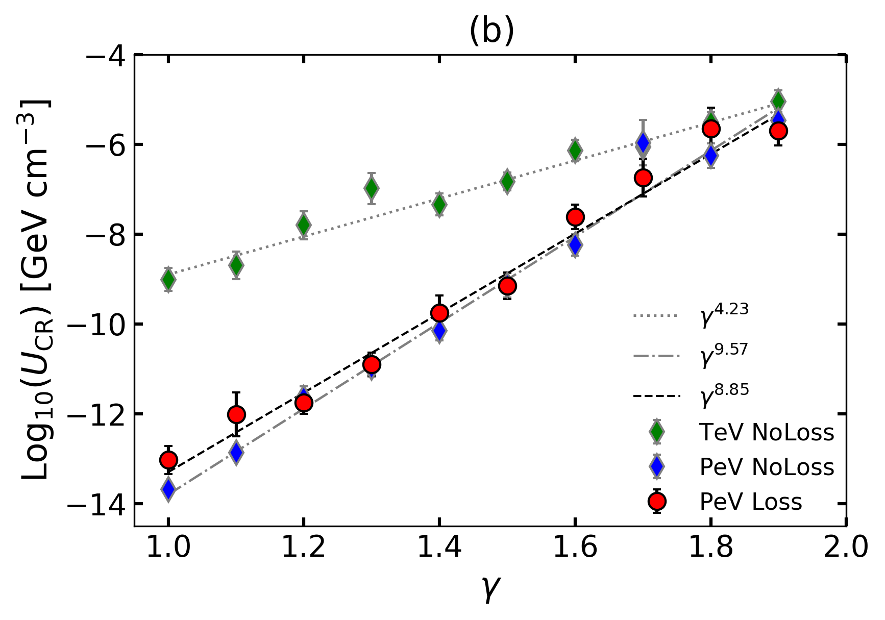
Similarly, we study the correlation between the averaged and turbulence index . Adopting the mono-energy injection with/without radiative losses, Fig. 8(b) shows the relation of , where the fitting index (GeV; not shown), 4.23 (TeV; without losses), 9.57 (PeV; without losses), and 8.85 (PeV; with losses). On the one hand, the relation between the averaged and strongly depends on the energy of particles, that is, the higher the energy is, the steeper the fitting index. On the other hand, radiation losses tend to slightly weaken the correlation between the averaged and .
Moreover, we want to explore to what extent the important power-law relations, i.e., Eqs. (2) and (3), associated with MHD turbulence properties, could maintain its own characteristics during the evolution process. We plot the ratio of the perpendicular diffusion coefficient to the parallel one as a function of the magnetization parameter (Fig. 8(c)), and the spatial diffusion (including and ) as the averaged energy (Fig. 8(d))555Note that we numerically calculate the parallel and perpendicular coefficient via and , respectively, where and are the evolution time and initial time, respectively., where the parameter denotes the energy averaged over both the evolution time and the number of particles in the evolution domain. As seen in Fig. 8(c), the ratio is related to the magnetization parameter by the power-law relations of in the sub-Alfvénic regime, and in the super-Alfvénic one. This numerical finding can well match the initial setting of , with the index 4 and 3. We demonstrate that during the long evolution time, the relation between the ratio and is independent of both radiative losses and kinetic energy of particles, suggesting that this relationship is an inherent property of particle transport in the magnetic turbulent environment. This implies that the anisotropy properties of MHD turbulence exclusively determine the anisotropic diffusion of CRs.
As for Fig. 8(d), we use the mono-energy injection of Group with the fixed = 5/3 and = 0.51, considering ten sets of the injection energy of particles range from to GeV with an interval of . For the non-loss case, the parallel diffusion coefficient (green thin-diamonds) and the perpendicular one (orange thin-diamonds) both present well a power-law relation of . While for the case with losses, the energy losses of high energy particles are more serious. We can see from this panel that the average energy distributed in the TeV region after the evolution of particles with energies above TeV. Even considering the radiative losses, (red circles) and (blue circles) still present well with the power-law relation of . It is in good agreement with the expected energy-dependent diffusion process. Consequently, the robust relations of (see Eq. (3)), and (see Eq. (2)) can be applied to understand the TeV and PeV gamma-ray emissions observed and predict the potential observational phenomenon.
5 Discussion
Through numerically solving the CR transport equation in a Crab-like nebula environment, we explored the interaction of high-energy CR electrons with magnetic turbulence in the framework of an anisotropic diffusion model. Specifically, regarding the magnetization parameter and turbulence spectral index as the adjustable parameters, we explore their influence on CR spectral, spatial diffusion, and anisotropy morphology.
The propagation process of CRs can be described with the time-dependent Fokker-Planck equation (Gaisser 1990; Berezinskii et al. 1990; Schlickeiser 2002). Provided that one considers different simplifications, the transport equation can be solved analytically (Webber et al. 1992; Maurin et al. 2002; Shibata et al. 2004). However, this simplification process may lead to the loss of CR propagation information. Therefore, the numerical/simulation approach is the main channel for revealing the CR propagation. At present, there are a number of numerical codes developed, e.g., GALPROP (Strong & Moskalenko 1998; Moskalenko & Strong 1998), PICARD (Kissmann 2014), DRAGON (Evoli et al. 2008), CRPROPA (Merten et al. 2017), and CRIPTIC (Krumholz et al. 2022), to understand CR observations. In the current work, we explored the diffusion properties of CRs using the CRIPTIC code, which is a new code for calculating both CR transport and observable emission.
In the framework of anisotropic diffusion, we investigated the influence of the magnetization parameter and turbulence index on the CR spatial distributions. In the sub-Alfvénic regime, we found that the resulting morphology and size of CR spatial distribution are consistent with that of emission images (Liu et al. 2019; De La Torre Luque et al. 2022) within small viewing angles, while in the case of super-Alfvénic turbulence, similar spatial distributions are also formed in the direction perpendicular to the mean magnetic field. Note that the stronger the anisotropy, the larger is, and the smaller the spatial extent, the larger . Therefore, when changing the viewing angle with both the large and , the expected spatial structures can be reproduced. For instance, with in the super-Alfvénic turbulence666This work mainly focuses on the strong turbulence region, that is, the spatial scale is smaller than the transition scale . For instance, considering the magnetic field strength of 50 G (corresponding to the super-Alfvénic regime) and the maximal energy of CRs of 10 PeV, we can simply estimate the maximal gyroradius of CRs with a velocity of as (Barreto-Mota et al. 2024) , which is much smaller than the parallel diffusion scales hundreds of pc, as seen in Fig. 4(c) for one super-Alfvénic case. Given such a small gyroradius, CR diffusion is strongly subjected to the anisotropy of magnetic fields., when , the parallel diffusion coefficient is about hundreds of times lower than the perpendicular one. This provides an alternative way for explaining the slow diffusion and morphology of observed TeV halos, with the LOS approximately aligned with the mean magnetic field.
For the other plausible explanation of the slow diffusion, i.e., the mirror diffusion, Lazarian & Xu (2021) analytically predicted the mirror diffusion is generally slower than the diffusion of non-bouncing CRs with small pitch angles between the local mean magnetic field and velocity of particles that undergo gyroresonant scattering. Subsequently, many numerical studies focused on exploring the diffusion and acceleration properties of CRs in the frame of mirror diffusion (e.g., Xu 2021; Xu & Li 2023; Zhang & Xu 2023, 2024; Barreto-Mota et al. 2024). They found that the mirror diffusion of CRs with sufficiently large pitch angles can explain the slow diffusion around the CR source. CRs may stochastically undergo slow mirror and fast scattering diffusion in the Galactic diffuse medium away from CR sources. We also expect that the mirror diffusion may be a plausible explanation for the slow diffusion near the source, which needs further research.
In the current work, in addition to the continuous injection used throughout this paper, we also tested the case of instantaneous, finding that CR’s overall evolution is similar to the continuous one. The only difference is the lack of the power-law relationship between the energy density and the effective radius. We also tested the streaming interaction for a wide distribution of CR energy (up to 10 PeV) and found that the streaming interaction almost does not change our results. We note that the streaming affects only the diffusion of the GeV CRs (see also the review Cesarsky (1980) and Farmer & Goldreich (2004) for the theoretical expectation). Therefore, the results we presented in the current work do not consider the streaming interaction. Since our study focuses on the CR electrons, it is enough to take the cooling effects of synchrotron radiation and IC scattering into account. When studying diffusion processes of the CR protons, one has to consider more cooling effects such as the coulomb, ionization, bremsstrahlung, and positron annihilation. Considering the PWN environment as a general research object, this work mainly focused on understanding how CR electrons interact with turbulent magnetic fields. Studies explaining real observations will be discussed elsewhere.
6 Summary
Considering PWN as a general research case in this paper, we numerically study the interactions of CRs with the ambient turbulent magnetic field. Focusing on the CR spectral distribution, anisotropy morphology, and spatial diffusion coefficients, our work is devoted to understanding CR propagation processes in the presence of magnetic turbulence. The main findings are briefly summarized as follows:
-
1.
We find that the energy density without radiative losses displays the power-law relationships of and , which are modified as and in the presence of radiative losses, respectively.
-
2.
The morphology of the CR spatial distribution strongly depends on the properties of turbulence. Namely, the magnetization parameter affects the spatial anisotropic distribution, while the turbulence spectral index its spatial extent. Note that the viewing angle also affects the spatial anisotropic distribution, consistent with the previous studies (e.g., Liu et al. 2019; De La Torre Luque et al. 2022).
-
3.
The CR electrons suffer from a slow diffusion near the source and a fast/normal diffusion away from the source. The effect of radiative losses, which happen far from the source, can suppress CR diffusion processes, resulting in a sub-diffusion behavior.
-
4.
The averaged energy density distributes a power-law relationship of , independent of both CR kinetic energy and radiative losses.
-
5.
Our simulation demonstrates that the relations of and maintain their features throughout a long evolution period. Since these two relations establish a robust connection between turbulent magnetic fields and CR diffusion coefficients, one can apply them to understand complex astrophysical processes related to turbulence cascades.
Acknowledgements.
We appreciate Mark R. Krumholz’s helpful discussions. The authors thank the support from the National Natural Science Foundation of China (grant No. 12473046). J.F.Z. also thanks the Hunan Natural Science Foundation for Distinguished Young Scholars (No. 2023JJ10039) and the China Scholarship Council for overseas research funds.References
- Abeysekara et al. (2017) Abeysekara, A. U., Albert, A., Alfaro, R., et al. 2017, Science, 358, 911
- Aguilar et al. (2016) Aguilar, M., Ali Cavasonza, L., Ambrosi, G., et al. 2016, Phys. Rev. Lett., 117, 231102
- Armillotta et al. (2022) Armillotta, L., Ostriker, E. C., & Jiang, Y.-F. 2022, ApJ, 929, 170
- Barreto-Mota et al. (2024) Barreto-Mota, L., de Gouveia Dal Pino, E. M., Xu, S., & Lazarian, A. 2024, arXiv e-prints, arXiv:2405.12146
- Beresnyak (2019) Beresnyak, A. 2019, Living Reviews in Computational Astrophysics, 5, 2
- Beresnyak et al. (2011) Beresnyak, A., Yan, H., & Lazarian, A. 2011, ApJ, 728, 60
- Berezinskii et al. (1990) Berezinskii, V. S., Bulanov, S. V., Dogiel, V. A., & Ptuskin, V. S. 1990, Astrophysics of cosmic rays
- Blasi (2013) Blasi, P. 2013, A&A Rev., 21, 70
- Caballero-Lopez et al. (2004) Caballero-Lopez, R. A., Moraal, H., McCracken, K. G., & McDonald, F. B. 2004, Journal of Geophysical Research (Space Physics), 109, A12102
- Cao et al. (2024) Cao, Z., Aharonian, F., An, Q., et al. 2024, ApJS, 271, 25
- Cao et al. (2021) Cao, Z., Aharonian, F. A., An, Q., et al. 2021, Nature, 594, 33
- Castellina & Donato (2005) Castellina, A. & Donato, F. 2005, Astroparticle Physics, 24, 146
- Cerri et al. (2021) Cerri, S. S., Arzamasskiy, L., & Kunz, M. W. 2021, ApJ, 916, 120
- Cesarsky (1980) Cesarsky, C. J. 1980, ARA&A, 18, 289
- Chandran (2000) Chandran, B. D. G. 2000, Phys. Rev. Lett., 85, 4656
- Cho & Lazarian (2002) Cho, J. & Lazarian, A. 2002, Phys. Rev. Lett., 88, 245001
- De La Torre Luque et al. (2022) De La Torre Luque, P., Fornieri, O., & Linden, T. 2022, Phys. Rev. D, 106, 123033
- Dempers & Engelbrecht (2020) Dempers, N. & Engelbrecht, N. E. 2020, Advances in Space Research, 65, 2072
- Elmegreen & Scalo (2004) Elmegreen, B. G. & Scalo, J. 2004, ARA&A, 42, 211
- Evoli et al. (2008) Evoli, C., Gaggero, D., Grasso, D., & Maccione, L. 2008, J. Cosmology Astropart. Phys., 2008, 018
- Evoli et al. (2012) Evoli, C., Gaggero, D., Grasso, D., & Maccione, L. 2012, Phys. Rev. Lett., 108, 211102
- Evoli et al. (2018) Evoli, C., Linden, T., & Morlino, G. 2018, Phys. Rev. D, 98, 063017
- Fang et al. (2019a) Fang, K., Bi, X.-J., & Yin, P.-F. 2019a, MNRAS, 488, 4074
- Fang et al. (2019b) Fang, K., Bi, X.-J., & Yin, P.-F. 2019b, ApJ, 884, 124
- Fang et al. (2018) Fang, K., Bi, X.-J., Yin, P.-F., & Yuan, Q. 2018, ApJ, 863, 30
- Fang et al. (2023) Fang, K., Hu, H.-B., Bi, X.-J., & Chen, E.-S. 2023, Phys. Rev. D, 108, 023017
- Farmer & Goldreich (2004) Farmer, A. J. & Goldreich, P. 2004, ApJ, 604, 671
- Gaggero et al. (2014) Gaggero, D., Maccione, L., Grasso, D., Di Bernardo, G., & Evoli, C. 2014, Phys. Rev. D, 89, 083007
- Gaisser (1990) Gaisser, T. K. 1990, Cosmic rays and particle physics.
- Gao & Zhang (2024) Gao, N.-N. & Zhang, J.-F. 2024, ApJ, 961, 80
- Goldreich & Sridhar (1995) Goldreich, P. & Sridhar, S. 1995, ApJ, 438, 763
- Grenier et al. (2015) Grenier, I. A., Black, J. H., & Strong, A. W. 2015, ARA&A, 53, 199
- Heesen et al. (2019) Heesen, V., Buie, E., I., Huff, C. J., et al. 2019, A&A, 622, A8
- Holod et al. (2005) Holod, I., Zagorodny, A., & Weiland, J. 2005, Phys. Rev. E, 71, 046401
- Hooper et al. (2017) Hooper, D., Cholis, I., Linden, T., & Fang, K. 2017, Phys. Rev. D, 96, 103013
- Hopkins et al. (2022) Hopkins, P. F., Butsky, I. S., Panopoulou, G. V., et al. 2022, MNRAS, 516, 3470
- Hu et al. (2022) Hu, Y., Lazarian, A., & Xu, S. 2022, MNRAS, 512, 2111
- Jokipii & Parker (1969) Jokipii, J. R. & Parker, E. N. 1969, ApJ, 155, 777
- Kempski & Quataert (2022) Kempski, P. & Quataert, E. 2022, MNRAS, 514, 657
- Kissmann (2014) Kissmann, R. 2014, Astroparticle Physics, 55, 37
- Kolmogorov (1941) Kolmogorov, A. 1941, Akademiia Nauk SSSR Doklady, 30, 301
- Kóta & Jokipii (2000) Kóta, J. & Jokipii, J. R. 2000, ApJ, 531, 1067
- Kraichnan (1965) Kraichnan, R. H. 1965, Physics of Fluids, 8, 1385
- Krumholz et al. (2022) Krumholz, M. R., Crocker, R. M., & Sampson, M. L. 2022, MNRAS, 517, 1355
- Krumholz et al. (2020) Krumholz, M. R., Crocker, R. M., Xu, S., et al. 2020, MNRAS, 493, 2817
- Lazarian & Xu (2021) Lazarian, A. & Xu, S. 2021, ApJ, 923, 53
- Lazarian & Yan (2014) Lazarian, A. & Yan, H. 2014, ApJ, 784, 38
- Li et al. (2024) Li, A.-f., Yuan, Q., Liu, W., & Guo, Y.-q. 2024, ApJ, 962, 43
- Linden & Buckman (2018) Linden, T. & Buckman, B. J. 2018, Phys. Rev. Lett., 120, 121101
- Liu & Yan (2020) Liu, R.-Y. & Yan, H. 2020, MNRAS, 494, 2618
- Liu et al. (2019) Liu, R.-Y., Yan, H., & Zhang, H. 2019, Phys. Rev. Lett., 123, 221103
- López-Coto et al. (2022) López-Coto, R., de Oña Wilhelmi, E., Aharonian, F., Amato, E., & Hinton, J. 2022, Nature Astronomy, 6, 199
- Lu et al. (2023) Lu, F.-W., Zhu, B.-T., Hu, W., & Zhang, L. 2023, ApJ, 953, 116
- Maiti et al. (2022) Maiti, S., Makwana, K., Zhang, H., & Yan, H. 2022, ApJ, 926, 94
- Manconi et al. (2020) Manconi, S., Di Mauro, M., & Donato, F. 2020, Phys. Rev. D, 102, 023015
- Maurin et al. (2002) Maurin, D., Taillet, R., & Donato, F. 2002, A&A, 394, 1039
- Merten et al. (2017) Merten, L., Becker Tjus, J., Fichtner, H., Eichmann, B., & Sigl, G. 2017, J. Cosmology Astropart. Phys., 2017, 046
- Michałek & Ostrowsky (1996) Michałek, G. & Ostrowsky, M. 1996, Nonlinear Processes in Geophysics, 3, 66
- Moskalenko & Strong (1998) Moskalenko, I. V. & Strong, A. W. 1998, ApJ, 493, 694
- Mukhopadhyay & Linden (2022) Mukhopadhyay, P. & Linden, T. 2022, Phys. Rev. D, 105, 123008
- Ostrowski & Siemieniec-Oziȩbło (1997) Ostrowski, M. & Siemieniec-Oziȩbło, G. 1997, Astroparticle Physics, 6, 271
- Parrish & Stone (2005) Parrish, I. J. & Stone, J. M. 2005, ApJ, 633, 334
- Parrish et al. (2008) Parrish, I. J., Stone, J. M., & Lemaster, N. 2008, ApJ, 688, 905
- Qiao et al. (2023) Qiao, B.-Q., Guo, Y.-Q., Liu, W., & Bi, X.-J. 2023, ApJ, 956, 75
- Recchia et al. (2021) Recchia, S., Di Mauro, M., Aharonian, F. A., et al. 2021, Phys. Rev. D, 104, 123017
- Schlickeiser (2002) Schlickeiser, R. 2002, Cosmic Ray Astrophysics
- Seo & Ptuskin (1994) Seo, E. S. & Ptuskin, V. S. 1994, ApJ, 431, 705
- Shibata et al. (2004) Shibata, T., Hareyama, M., Nakazawa, M., & Saito, C. 2004, ApJ, 612, 238
- Sioulas et al. (2020) Sioulas, N., Isliker, H., Vlahos, L., Koumtzis, A., & Pisokas, T. 2020, MNRAS, 491, 3860
- Strong & Moskalenko (1998) Strong, A. W. & Moskalenko, I. V. 1998, ApJ, 509, 212
- Strong et al. (2007) Strong, A. W., Moskalenko, I. V., & Ptuskin, V. S. 2007, Annual Review of Nuclear and Particle Science, 57, 285
- Tang & Piran (2019) Tang, X. & Piran, T. 2019, MNRAS, 484, 3491
- Trotta et al. (2011) Trotta, R., Jóhannesson, G., Moskalenko, I. V., et al. 2011, ApJ, 729, 106
- Webber et al. (1992) Webber, W. R., Lee, M. A., & Gupta, M. 1992, ApJ, 390, 96
- Wiener et al. (2017) Wiener, J., Pfrommer, C., & Oh, S. P. 2017, MNRAS, 467, 906
- Xi et al. (2019) Xi, S.-Q., Liu, R.-Y., Huang, Z.-Q., Fang, K., & Wang, X.-Y. 2019, ApJ, 878, 104
- Xiao et al. (2024) Xiao, Y.-W., Zhang, J.-F., & Xu, S. 2024, submitted to A&A
- Xu (2021) Xu, S. 2021, ApJ, 922, 264
- Xu & Li (2023) Xu, S. & Li, H. 2023, ApJ, 957, 97
- Xu & Yan (2013) Xu, S. & Yan, H. 2013, ApJ, 779, 140
- Yan & Lazarian (2002) Yan, H. & Lazarian, A. 2002, Phys. Rev. Lett., 89, 281102
- Yan & Lazarian (2008) Yan, H. & Lazarian, A. 2008, ApJ, 673, 942
- Yan et al. (2012) Yan, H., Lazarian, A., & Schlickeiser, R. 2012, ApJ, 745, 140
- Yan et al. (2024) Yan, K., Liu, R.-Y., Zhang, R., et al. 2024, Nature Astronomy, 8, 628
- Zhang & Xu (2023) Zhang, C. & Xu, S. 2023, ApJ, 959, L8
- Zhang & Xu (2024) Zhang, C. & Xu, S. 2024, arXiv e-prints, arXiv:2406.03542
- Zhang et al. (2018) Zhang, J.-F., Li, Z.-R., Xiang, F.-Y., & Lu, J.-F. 2018, MNRAS, 473, 3211
- Zhang & Xiang (2021) Zhang, J.-F. & Xiang, F.-Y. 2021, ApJ, 922, 209
- Zyuzin et al. (2021) Zyuzin, D. A., Karpova, A. V., Shibanov, Y. A., Potekhin, A. Y., & Suleimanov, V. F. 2021, MNRAS, 501, 4998
Appendix A The main procedures of our simulation experiments
Lazarian & Yan (2014) analytically predicted the potential relation between the ratio of the perpendicular diffusion coefficient to the parallel component and the magnetization parameter of
| (4) |
in the strong turbulence range, where 4.0 for the sub-Alfvénic turbulence and 3.0 for the super-Alfvénic case. This relation has been verified by the test-particle simulations (Xu & Yan 2013; Maiti et al. 2022). However, analytical and numerical studies did not consider the possible effect of both the change of CR energies and their radiative losses on the power-law relation. We note that some works, such as Liu et al. (2019) and De La Torre Luque et al. (2022), directly used the relation of to explain the slow diffusion phenomena. One of the motivations of the current work is to explore whether the relationship between the ratio of the spatial diffusion coefficient and the magnetization parameter can maintain its properties during the propagation process of CRs.
To conduct our simulations using the CRIPPTIC code, we need to obtain the input parameters that the CRIPPTIC code can invoke, by setting some physical parameters related to MHD turbulence dynamics and CRs. For an example of our simulations, which considers the case of GeV with radiative loss processes (including synchrotron radiative losses due to the presence of the ISM magnetic field and IC scattering losses due to both interstellar radiation field with a temperature of 20 K and cosmic microwave one in the Klein-Nishina regime), we describe the main procedures as follows.
: Since CRIPTIC takes the sub-grid values for diffusion coefficients as input parameters, needs to be taken as the baseline value. With the energy-dependent parallel diffusion coefficient (Seo & Ptuskin 1994; Trotta et al. 2011; Dempers & Engelbrecht 2020)
| (5) |
where and are the mass of the electron and light speed, respectively, we first obtain the initial parallel diffusion coefficient . Note that the CRIPTIC code considers the normalized spatial diffusion coefficient , diffusion index , and the kinetic energy of electrons as input parameters. In this case, we fixed for ISM diffusion (Heesen et al. 2019) and considered a power-law energy distribution of with . By setting the parameter , we can obtain a connection between the diffusion index and magnetic turbulence index (for instance, setting , we have corresponding to the Kolmogorov-type turbulence; see more details in Sect. 2.1).
: On the basis of the established in Step 1, we can constrain the initial perpendicular diffusion coefficient via 4. We note that the CRIPTIC code parameterizes the ratio of as . In this work, we define to establish the link between the ratio of and the magnetization parameter . Given theoretical expectation and numerical confirmation of the index value mentioned above, we fixed 4.0 for the sub-Alfvénic turbulence and 3.0 for the super-Alfvénic one. For the magnetization parameter, i.e., the Alfvén Mach number , we controlled its value by regulating the mean magnetic field strength along with the -axis direction, considering a uniform region containing gas with a density of and velocity of .
: Furthermore, we use the established parallel diffusion coefficient in Step 1 to obtain the initial energy diffusion coefficient by (Michałek & Ostrowsky 1996).
Based on this framework, we explore the interaction of high-energy CR electrons with magnetic turbulence, regarding the magnetization parameter (in the range of [0, 3]), turbulence spectral index ( in the range of [1.0, 1.9], i.e., [0.1, 1.0]), and particle’s energy (in the range of [, ] GeV) as free parameters, together with the radiative processes, and divide our simulations into three groups. The detailed parameters of each group are provided in Sect. 3.