Anisotropic Andreev reflection in semi-Dirac materials
Abstract
In the framework of Bogoliubov-de Gennes equation, we theoretically study the Andreev reflection in normal-superconducting junctions based on semi-Dirac materials. Owing to the intrinsic anisotropy of semi-Dirac materials, the configuration of Andreev reflection and differential conductance are strongly orientation-dependent. For the transport along the linear dispersion direction, the differential conductance exhibits a clear crossover from retro Andreev reflection to specular Andreev reflection with an increasing bias-voltage, and the differential conductance oscillates without a decaying profile when the interfacial barrier strength increases. However, for the transport along the quadratic dispersion direction, the boundary between the retro Andreev reflection and specular Andreev reflection is ambiguous, and the differential conductance decays with increasing the momentum mismatch or the interfacial barrier strength. We illustrate the pseudo-spin textures to reveal the underling physics behind the anisotropic coherent transport properties. These results enrich the understanding of the superconducting coherent transport in semi-Dirac materials.
I Introduction
Semi-Dirac material (SDM) has recently been experimentally realized in black phosphorus with in situ deposition of K Kim et al. (2015) or Rb Kim et al. (2017) atoms, offering a promising playground for further exploring the exotic attributes of SDMs. Unlike most Dirac materials that possess liner dispersions in all momentum-space directions Castro Neto et al. (2009); Wehling et al. (2014); Armitage et al. (2018), in SDMs the low-energy excitations disperse quadratically in one direction but linearly along the orthogonal direction Pardo and Pickett (2009); Zhong et al. (2017); Pardo and Pickett (2009); Huang et al. (2015); Dietl et al. (2008); Delplace and Montambaux (2010). The unique band structures of SDMs are responsible for a series of novel phenomena Dietl et al. (2008); Delplace and Montambaux (2010); Saha et al. (2017); Banerjee and Pickett (2012); Nualpijit et al. (2018); Mawrie and Muralidharan (2019a); Adroguer et al. (2016); Islam and Saha (2018); Mawrie and Muralidharan (2019b); Carbotte and Nicol (2019); Real et al. (2020); Chen et al. (2018); Zhai and Wang (2014); Wang et al. (2017); Saha (2016); Dutreix et al. (2013), including the consequences of anisotropic aspect in the superconducting order parameter correlations Wang et al. (2019); Uchoa and Seo (2017); Uryszek et al. (2019). Recent theoretical efforts have demonstrated that the superconductivity in SDMs can be induced by arbitrarily weak attractions in the present of random chemical potential Wang et al. (2019). Resorting to the mean-field calculation Uchoa and Seo (2017) and renormalization group analysis Uryszek et al. (2019), it is revealed that the s-wave superconductivity is more favorable in SDMs. More strikingly, owing to the intrinsic anisotropy, the stiffness of superconducting order parameter and the divergence behavior of correlation length are highly orientation-dependent Uchoa and Seo (2017); Uryszek et al. (2019). These progresses, together with the developments in the materialization of SDMs, provide foundations for exploring coherent transport properties in SDM-based normal-superconducting (NS) junctions.
In a NS junction with ideal contacts, the transport properties are dominated by the Andreev reflection (AR) in the subgap energy regime of , with the incident energy and the superconducting gap Andreev (1964); Pannetier and Courtois (2000). In most conventional-metal-based NS junctions, the chemical potential in the N region satisfies , and the AR is a intra-band phase-coherent scattering process, during which an incident electron from the N region is reto-reflected as a hole Andreev (1964); Pannetier and Courtois (2000); Zhu et al. (1999); Blonder et al. (1982). While in the NS junctions based on Dirac materials, can be continuously tuned to the subgap regime satisfying Castro Neto et al. (2009); Wehling et al. (2014); Beenakker (2008). Consequently, a conduction-band electron incident from the N region is specularly reflected back as a valence-band hole, leading to a inter-band phase-coherent scattering process known as specular-AR Beenakker (2008, 2006); Bhattacharjee and Sengupta (2006); Linder and Yokoyama (2014); Li (2016); Ludwig (2007); Efetov and Efetov (2016). Remarkably, by increasing within the subgap regime, a crossover from reto-AR to specular-AR occurs, manifesting itself as a dip at in the -dependent conductance spectrum. This signature has been experimentally observed in bilayer-graphene-based NS junctions Efetov et al. (2016). Moreover, in Dirac-material-based NS junction, due to the novel momentum-spin/pseudo-spin textures of Dirac fermions, the subgap differential conductance oscillates with the interfacial barrier strength without a decay profile Bhattacharjee and Sengupta (2006).
Although the scenarios of AR in the systems with pure quadratic Andreev (1964); Pannetier and Courtois (2000); Zhu et al. (1999); Blonder et al. (1982) or linear Beenakker (2006); Bhattacharjee and Sengupta (2006); Linder and Yokoyama (2014); Li (2016); Beenakker (2008); Ludwig (2007); Efetov and Efetov (2016) dispersions have triggered extensive studies, the AR and related subgap conductance in SDM-based NS junctions have received no attention to date. Since the low-energy excitations in SDMs host unique dispersions intermediate between the quadratic and linear energy spectra, it is natural to ask how the intrinsic anisotropy manifests itself in the superconducting coherent transport. In this paper we investigate the subgap transport properties in SDM-based NS junctions. The manifestations of the anisotropic dispersion in the subgap transport can be summarized as two points. First, we find a clear crossover from retro-AR to specular-AR when the transport along the linearly dispersion direction, while for the transport along the quadratical dispersion direction, the boundary between retro-AR and specular-AR is ambiguous. Second, the influences of momentum-mismatch and interfacial barrier on the subgap transport are strongly orientation-dependent. For the transport along the quadratic dispersion direction, the subgap differential conductance rapidly decays with increasing the interfacial barrier strength or momentum-mismatch between the N and S regions. Whereas the transport in the linear dispersion direction is insensitive to the momentum-mismatch, and the subgap differential conductance periodically oscillates with the interfacial barrier strength without a decaying profile. We illustrate the pseudo-spin textures of semi-Dirac fermions to understand our findings.
II Model and Method
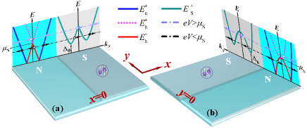
To address the effects of the intrinsic anisotropy on the subgap transport properties, we introduce two representative SDM-based NS junctions extending along the - and - axes, respectively. As schematically shown in Fig. 1, the low-energy dispersion is linear (quadratic) in the N region of the NS junction extending along the -axis. We consider the transport properties along the -direction in the NS junction extending along the -axis, and assume that the translational symmetry in the -direction is preserved, so that the transverse momentum can be treated as a good quantum number Beenakker (2006, 2008); Bhattacharjee and Sengupta (2006); Ludwig (2007); Linder and Yokoyama (2014); Li (2016); Efetov and Efetov (2016). Moreover, under this assumption the influences of boundary effects on the transport can be rationally neglected. In the S region, we take the intra-sublattice/orbit s-wave pairing, as proposed by recent theoretical work Uchoa and Seo (2017); Uryszek et al. (2019). In practice, the superconductivity in the S region can be induced by a s-wave superconductor via the proximity effect, as implemented in similar NS junctions based on graphene Heersche et al. (2007); Efetov et al. (2016) and Weyl semimetals Bachmann et al. (2017); Huang et al. (2018).
Under these lines, the Bogoliubov–de Gennes (BdG) Hamiltonian describing the low-lying physics is given by Uchoa and Seo (2017); Uryszek et al. (2019)
| (1) |
acting on the pseudo-spin Nambu space. The single-particle effective Hamiltonian , where label the Pauli matrices operating on the pseudo-spin space, represents the Fermi velocity, and with the effective mass. The chemical potential , where is the Heaviside step function and () denotes the chemical potential in the S (N) region. In this paper, we assume that the relation of is satisfied, so that the leakage of Cooper pairs from the S to N regions can be safely neglected Beenakker (2006); Bhattacharjee and Sengupta (2006); Ludwig (2007); Linder and Yokoyama (2014); Li (2016); Efetov and Efetov (2016) . In doing so, the pair potential can be effectively modeled by a step function, i.e., , with the superconducting phase and a identity matrix operating on the pseudo-spin space. The BdG Hamiltonian shown in Eq. (1) can also be derived from the lattice model of a graphene-like system in proximity to a s-wave superconductor. The related calculation details are given in Appendix A.
By diagonalizing the Hamiltonian shown in Eq. (1) straightforwardly, the energy dispersion in the S region can be written as
| (2) |
where and indicate the different branches. To ensure the validity of mean-field approximation, the relation of should be satisfied. Therefore, the branches are far away from the subgap regime and only bands need to be considered. The schematic plots of as functions of and are shown in Fig. 1 (a) and (b), respectively. In the N region, the low-energy spectrum can be formulated as
| (3) |
where the subscripts and denote the electronlike and holelike excitation spectra, respectively.
According to Eq. (3), the group velocities in the N region can be parameterized as
| (4) |
where . The components and exhibit distinct behaviors with respect to the momentum, reflecting the anisotropic aspect of SDMs. We note that due to the intrinsic anisotropy, in the scattering issues the scattering angle should be defined as one between the directions of associated group velocity and current, instead of the angle between the directions of momentum and current. Resorting to Eq. (4), for a NS junction extending along the -axis, the scattering angle should be , differing from the angle of in isotropic systems Beenakker (2006); Bhattacharjee and Sengupta (2006); Linder and Yokoyama (2014); Li (2016). For a NS junction extending along the -axis, the scattering angle .
II.1 NS junction extending along the -axis
We now turn to the scattering problem in a NS junction extending along the -axis. In practice, at the boundary between the N and S regions, the defects and lattice mismatch are inevitable during the fabrication of device, which may profoundly influence the transport properties. To take into account the proposed effects, we introduce a interfacial barrier , and take the limit of and with being finite. We note that in the current direction, the low-energy excitations in SDMs are similar as that in Dirac materials, thus the scattering amplitudes can be calculated by the standard procedure employed in related Dirac-material-based NS junctions Beenakker (2006, 2008); Bhattacharjee and Sengupta (2006); Ludwig (2007); Linder and Yokoyama (2014); Li (2016); Efetov and Efetov (2016). By solving
| (5) |
at the boundary of , we can obtain and , which are the reflection amplitude for the AR (normal reflection) and the transmission amplitude for the electron(hole)-like quasiparticle, respectively. The details of basis scattering states and are, respectively, given by Eqs. (26b) and (28b). The transfer matrix , with a identity matrix operating on the Nambu space.
In the limit regime of , the reflection amplitudes are, respectively, given by
| (6a) | |||
| (6b) |
where , , and . As can be seen, both and are independent of , implying that in the limit of , the transport properties along the -axis direction are insensitive to the interfacial barrier.
Resorting to the reflection amplitudes, the probabilities for the normal reflection (NR) and AR processes can be, respectively, defined as
| (7a) | |||
| (7b) |
where the particle current density operator , with the Pauli matrix operating on the Nambu space.
Taking advantage of the Blonder-Tinkham-Klapwijk (BTK) formula Blonder et al. (1982), the zero-temperature differential conductance along the -direction is given by
| (8) |
where indicates the bias voltage and is the width along the -direction of the junction. To normalize the conductance, we define , which is the conductance along the -direction of a SDM-based NN junction in the ballistic limit.
II.2 NS junction along the -axis
In a NS junction along the -axis, the low-energy excitations of the N region disperse quadratically in the current direction. For electron(hole)-like excitations with , Eq. (3) determines four possible scattering modes, including two propagating modes with and two evanescent ones with . The related parameters are given by
| (9a) | |||
| (9b) |
with . Although the evanescent modes do not contribute to the current, they need to be included in the wave functions to get correct boundary conditions. With this in mind, for a propagating electron-like incident mode, the wave function in the N region should be parameterized as
| (10) |
with and the reflection amplitudes of propagating and evanescent modes in the NR(AR) processes, respectively. The detailed structures of related basis scattering states are given by Eq. (30d). In the S region, the wave function takes the form of
| (11) |
where the associated basis scattering states are shown in Eq. (31b). The coefficients and , respectively, represent the transmission amplitudes for the propagating and evanescent electron(hole)-like quasiparticles.
To model the effects resulting from the interfacial defects and lattice mismatch, we introduce a interfacial barrier modeled by , with being the Delta function. In doing so, the boundary conditions can be formulated as
| (12a) | |||
| (12b) |
where . For brevity of notation, we introduce a parameter to characterize the interfacial barrier strength, with . The probabilities for the NR and AR processes are, respectively, defined as
| (13a) | |||
| (13b) |
with the particle current density operator . We note that the probabilities of evanescent modes and are vanishing and do not contribute to the current. Therefore, in accordance with the BTK formula Blonder et al. (1982), the zero-temperature differential conductance along the -direction can be written as
| (14) |
where is the width along the -direction of the junction. It is convenient to normalize the conductance by , which represents the conductance in the -direction of a SDM-based NN junction in the ballistic limit.

III Results and Discussion
III.1 Pseudo-spin Textures
To understand the underlying physics behind the transport properties, it is instructive to reveal the pseudo-spin textures in the N regions of SDMs-based NS junctions. To do so, we define the pseudo-spin vector as , which is a unit vector consisting of the expectation values of operator in normalized basis scattering states, where San-Jose et al. (2009); Schomerus (2010); Majidi and Zareyan (2011, 2011); Habe (2019). Specifically, the pseudo-spin carried by a propagating electron-like mode can be formulated as
| (15) |
Accordingly, the pseudo-spin components and depend, respectively, linearly and quadratically on the momentum, inheriting the intrinsic anisotropy of SDMs. Fig. 2 gives the schematic plots for the pseudo-spin textures of electron-like conduction band. As can be seen, is always along the positive -direction, regardless of the sign of , this scenario is profoundly different from that in Dirac materials San-Jose et al. (2009); Schomerus (2010); Majidi and Zareyan (2011, 2011); Habe (2019); Breunig et al. (2018); Uchida et al. (2014); Bai and Yang (2020). As will be proposed in Sec. III.2, the unique pseudo-spin textures provide illuminating elucidations for the subgap transport properties in SDMs-based NS junctions.
III.2 Differential conductance


In this subsection, we proceed to analyze the numerical results and discuss the differential conductance in the subgap regime. What we mainly concentrate on are the manifestations of the intrinsic anisotropy in the subgap transport properties, implemented by comparing the AR configurations and subgap differential conductance along the - and -axes. To ensure the validity of the mean-field approximation, we assume the S regions are heavily doped to the regime of , and we set in the numerical calculation for definiteness.
As a starting point, we focus on the bias-voltage-dependent subgap differential conductance, and analyze the results in terms of the unique pseudo-spin textures. In a NS junction extending along the -axis, the zero-bias conductance is insensitive to the momentum-mismatch (or alternatively, the ratio of ). As shown in Fig. 3, the differential conductance always exhibits a zero-bias peak, regardless of the value of . Remarkably, for any nonvanishing , takes the same value of . On the contrary, the strongly depends on the momentum-mismatch in the NS junction extending along the -axis. As can be seen in Fig. 3, the subgap differential conductance almost vanishes in the presence of large momentum-mismatch (e.g., ). Therefore, the behavior of zero-bias conductance is highly orientation-dependent. This scenario can be understood by virtue of the anisotropic pseudo-spin textures illustrated in Fig. 2. In the NS junction along the -direction, for a small (i.e., with a small incident angle), the pseudo-spin carried by an electron-like incident mode is nearly opposite to that of the normally reflected one. Consequently, when is small enough, the conservation of pseudo-spin results in the prohibition of NR, and thus leads to the enhancement of AR in the subgap regime, even in the presence of strong momentum-mismatch. Moreover, since the conductance is mainly contributed by the modes with small , the zero-bias conductance is insensitive to the momentum-mismatch. However, in the NS junction extending along the -direction, a couple of incident and normally reflected modes possess the same pseudo-spin, so that the back scattering is enabled. Therefore, the subgap differential conductance in the -direction is strongly suppressed by increasing the momentum-mismatch.


Parenthetically, although the configuration of shown in Fig. 3 is similar as that in associated NS junctions based on graphene Beenakker (2006) and silicene Linder and Yokoyama (2014); Li (2016), there is a significant difference on the value of . For , according to Eqs. (6b) and (7b), the reflection probabilities reduces into and , respectively. Substituting the results into Eq. (8), we arrive at , differing from the value of in graphene- and silicene-based NS junctions Beenakker (2006); Linder and Yokoyama (2014); Li (2016). This consequence can be ascribed to the unique band structure of SDMs intermediate the linear and quadratic spectra.


The anisotropic aspect of the subgap differential conductance also manifests itself in the distinct crossover behaviors from the retro-AR to specular-AR in the two representative NS junctions. In the NS junction with a weakly doped N region satisfying , the subgap differential conductance vanishes at , due to the absence of AR for any incident angles. Furthermore, in the regimes of and , the subgap differential conductance is dominated by the retro-AR and specular-AR, respectively. Therefore, the point of serves as the crossover boundary between the retro-AR and specular-AR in the subgap regime. In the NS junction along the -axis, as the bias-voltage increases, the subgap differential conductance exhibits a clear crossover from retro-AR to specular-AR, as depicted by Fig. 4. However, as illustrated in Fig. 4, the boundary between retro-AR and specular-AR is ambiguous in the NS junction extending along the -axis. This scenario can be understood from the unique pseudo-spin textures. In the NS junction extending in the -axis, the incident and normally reflected modes carry the same pseudo-spin, thus the NR is favorable, especially in the presence of large momentum-mismatch. Consequently, as illustrated in Fig. 3 and the inset therein, for , the AR process is strongly suppressed so that in the subgap regime, thus blurring the boundary between the retro-AR and specular-AR.
We now turn to the effects of the interfacial barriers on the subgap differential conductance. For the transport along the -axis, the pseudo-spin carried by the incident and normally reflected modes are nearly opposite to each other when the incident angle is small enough, resulting in the prohibition of NR. As a consequence, the zero-bias differential conductance just oscillates with without a decaying profile, as charted out by Fig. 5. In the case of the NS junction extending along the -axis, the back scattering is available since the incident and normally reflected modes host the same pseudo-spin. Therefore, the AR is strongly suppressed by increasing the interfacial barrier strength, leading to the exponential decaying profile in the -dependent shown in Fig. 5. In this regard, the influences of the interfacial barrier on the subgap transport are orientation-dependent, reflecting the anisotropic aspect of SDMs.
IV Conclusion
In conclusion, we have studied the subgap transport properties in SDMs-based NS junctions in the framework of BdG equation. In terms of the tight-binding approach, the BdG Hamiltonian has been derived from a graphene-like system proximitized to a s-wave superconductor. We have figured out the manifestations of the intrinsic anisotropy of SDMs in the AR configurations and subgap differential conductance. For the transport along the linear dispersion direction, the subgap differential conductance exhibits a clear crossover from retro-AR to specular-AR by enhancing the bias-voltage, and the zero-bias differential conductance is insensitive to the momentum mismatch. Moreover, when the interfacial barrier strength increases, the zero-bias conductance exhibits an oscillating configuration without a decaying profile. However, for the transport along the quadratic dispersion direction, the boundary between the retro-AR and specular-AR is ambiguous, and the the zero-bias differential conductance rapidly drops as the momentum mismatch or the interfacial barrier strength increases. These results would provide some intriguing insights for the coherent transport in SDMs-based superconducting hybrid structures, and we anticipate more interesting results for the Andreev bound states and supercurrents in SDMs-based Josephson junctions.
Acknowledgements.
H. L. and X. H. would like to thank E. Rossi and R. Wang for helpful discussions. This work was supported by the National Natural Science Foundation of China (Grants No 11804091 and No. 91833302), the Science and Technology Planning Project of Hunan Province (Grant No. 2019RS2033), the Hunan Provincial Natural Science Foundation of China (Grant No. 2019JJ50380), and the excellent youth fund of the Hunan Provincial Education Department (Grant No. 18B014).Appendix A Derivation of the BdG Hamiltonian
Physically, the semi-Dirac dispersion can be realized in a graphene-like systems with breaking the hexagonal symmetry Chen et al. (2018); Zhong et al. (2017); Mawrie and Muralidharan (2019b). Thus we take an artificial honeycomb lattice model with anisotropic nearest-neighbor (NN) hopping as a prototype. The NN tight-binding model containing an intro-sublattice/orbit Bardeen-Cooper-Schrieffer superconducting pairing term is given by
| (16) |
where the primitive lattice vectors and with the interatomic distance, and for . Performing Fourier-transformations according to and , we arrive at
| (17) |
where the parameter is given by
| (18) |
with the NN lattice vectors being defined as , , and . Accordingly, the dispersion for the normal state is .
For the critical case of , vanishes at , and the normal state reaches the semi-Dirac phase. Now we linearize the Hamiltonian for a small around the point by setting and , with and being satisfied. Up to the second order in , we arrive at
| (19a) | |||
| (19b) | |||
| (19c) | |||
| (19d) |
Substituting Eq. (19d) into Eq. (17), we obtain the Hamiltonian at point as
| (20) | |||||
where the relation of has been used. Rewrite in the form of , with the basis
| (21) |
and
| (22) |
By defining , , and , the upper block can be formulated as
| (23) |
where the anticommutation relation has been employed. Taking a unitary transformation with
| (24) |
The BdG Hamiltonian can be compactly written as
| (25) |
where we rewrite with the amplitude of pairing potential and the superconducting phase, is a identity matrix, and the Pauli matrices and act on the pseudo-spin and Nambu spaces, respectively.
Appendix B Calculation of the basis scattering states in NS junctions based on semi-Dirac materials
In this appendix we present necessary calculation details regarding the wave functions and related quantities in SDMs-based NS junctions.
B.1 NS junction extending along the x-axis
For the NS junction extending along the -axis, we assume the translational symmetry is preserved in the direction, thus the transverse momentum can be treated as a good quantum number. In the S region, solving the BdG equation straightforwardly yields
| (26a) | |||
| (26b) |
where the related parameters are defined by
| (27a) | |||
| (27b) | |||
| (27c) | |||
| (27d) |
In the N region, the basis scattering states can be formulated as
| (28a) | |||
| (28b) |
In the interfacial barrier region, the -components of momenta . By substituting and , respectviely, with and into Eq. (28b), we obtain the basis scattering states in the interfacial barrier region. The related wave functions can be expressed as
| (29) |
where label the scattering amplitudes.
B.2 NS junction along the -axis
In the NS junction along the -direction, we assume the transverse momentum is preserved. In the N region, solving the BdG equation gives the basis states
| (30a) | |||
| (30b) | |||
| (30c) | |||
| (30d) |
In the S region, the basis states can be formulated as
| (31a) | |||
| (31b) |
with the associated parameters being defined as
| (32a) | |||
| (32b) | |||
| (32c) | |||
| (32d) | |||
| (32e) | |||
| (32f) |
We note that for , denote the electron(hole)-like scattering states propagating along the -directions, while represent the evanescent ones decaying exponentially as . In the case of , all scattering states given by Eq. (31b) describe the evanescent modes.
References
- Kim et al. (2015) J. Kim, S. S. Baik, S. H. Ryu, Y. Sohn, S. Park, B.-G. Park, J. Denlinger, Y. Yi, H. J. Choi, and K. S. Kim, Science 349, 723 (2015).
- Kim et al. (2017) J. Kim, S. S. Baik, S. W. Jung, Y. Sohn, S. H. Ryu, H. J. Choi, B.-J. Yang, and K. S. Kim, Phys. Rev. Lett. 119, 226801 (2017).
- Castro Neto et al. (2009) A. H. Castro Neto, F. Guinea, N. M. R. Peres, K. S. Novoselov, and A. K. Geim, Rev. Mod. Phys. 81, 109 (2009).
- Wehling et al. (2014) T. Wehling, A. Black-Schaffer, and A. Balatsky, Adv. Phys. 63, 1 (2014).
- Armitage et al. (2018) N. P. Armitage, E. J. Mele, and A. Vishwanath, Rev. Mod. Phys. 90, 015001 (2018).
- Pardo and Pickett (2009) V. Pardo and W. E. Pickett, Phys. Rev. Lett. 102, 166803 (2009).
- Zhong et al. (2017) C. Zhong, Y. Chen, Y. Xie, Y.-Y. Sun, and S. Zhang, Phys. Chem. Chem. Phys. 19, 3820 (2017).
- Huang et al. (2015) H. Huang, Z. Liu, H. Zhang, W. Duan, and D. Vanderbilt, Phys. Rev. B 92, 161115 (2015).
- Dietl et al. (2008) P. Dietl, F. Piéchon, and G. Montambaux, Phys. Rev. Lett. 100, 236405 (2008).
- Delplace and Montambaux (2010) P. Delplace and G. Montambaux, Phys. Rev. B 82, 035438 (2010).
- Saha et al. (2017) K. Saha, R. Nandkishore, and S. A. Parameswaran, Phys. Rev. B 96, 045424 (2017).
- Banerjee and Pickett (2012) S. Banerjee and W. E. Pickett, Phys. Rev. B 86, 075124 (2012).
- Nualpijit et al. (2018) P. Nualpijit, A. Sinner, and K. Ziegler, Phys. Rev. B 97, 235411 (2018).
- Mawrie and Muralidharan (2019a) A. Mawrie and B. Muralidharan, Phys. Rev. B 99, 075415 (2019a).
- Adroguer et al. (2016) P. Adroguer, D. Carpentier, G. Montambaux, and E. Orignac, Phys. Rev. B 93, 125113 (2016).
- Islam and Saha (2018) S. F. Islam and A. Saha, Phys. Rev. B 98, 235424 (2018).
- Mawrie and Muralidharan (2019b) A. Mawrie and B. Muralidharan, Phys. Rev. B 100, 081403 (2019b).
- Carbotte and Nicol (2019) J. P. Carbotte and E. J. Nicol, Phys. Rev. B 100, 035441 (2019).
- Real et al. (2020) B. Real, O. Jamadi, M. Milićević, N. Pernet, P. St-Jean, T. Ozawa, G. Montambaux, I. Sagnes, A. Lemaître, L. Le Gratiet, A. Harouri, S. Ravets, J. Bloch, and A. Amo, Phys. Rev. Lett. 125, 186601 (2020).
- Chen et al. (2018) Q. Chen, L. Du, and G. A. Fiete, Phys. Rev. B 97, 035422 (2018).
- Zhai and Wang (2014) F. Zhai and J. Wang, J. Appl. Phys. 116, 063704 (2014).
- Wang et al. (2017) J.-R. Wang, G.-Z. Liu, and C.-J. Zhang, Phys. Rev. B 95, 075129 (2017).
- Saha (2016) K. Saha, Phys. Rev. B 94, 081103 (2016).
- Dutreix et al. (2013) C. Dutreix, L. Bilteanu, A. Jagannathan, and C. Bena, Phys. Rev. B 87, 245413 (2013).
- Wang et al. (2019) J.-R. Wang, G.-Z. Liu, and C.-J. Zhang, J. Phys. Commun. 3, 055006 (2019).
- Uchoa and Seo (2017) B. Uchoa and K. Seo, Phys. Rev. B 96, 220503 (2017).
- Uryszek et al. (2019) M. D. Uryszek, E. Christou, A. Jaefari, F. Krüger, and B. Uchoa, Phys. Rev. B 100, 155101 (2019).
- Andreev (1964) A. F. Andreev, Sov. Phys. JETP 19, 1228 (1964).
- Pannetier and Courtois (2000) B. Pannetier and H. Courtois, J. Low Temp. Phys. 118, 599 (2000).
- Zhu et al. (1999) J.-X. Zhu, B. Friedman, and C. S. Ting, Phys. Rev. B 59, 9558 (1999).
- Blonder et al. (1982) G. E. Blonder, M. Tinkham, and T. M. Klapwijk, Phys. Rev. B 25, 4515 (1982).
- Beenakker (2008) C. W. J. Beenakker, Rev. Mod. Phys. 80, 1337 (2008).
- Beenakker (2006) C. W. J. Beenakker, Phys. Rev. Lett. 97, 067007 (2006).
- Bhattacharjee and Sengupta (2006) S. Bhattacharjee and K. Sengupta, Phys. Rev. Lett. 97, 217001 (2006).
- Linder and Yokoyama (2014) J. Linder and T. Yokoyama, Phys. Rev. B 89, 020504 (2014).
- Li (2016) H. Li, Phys. Rev. B 94, 075428 (2016).
- Ludwig (2007) T. Ludwig, Phys. Rev. B 75, 195322 (2007).
- Efetov and Efetov (2016) D. K. Efetov and K. B. Efetov, Phys. Rev. B 94, 075403 (2016).
- Efetov et al. (2016) D. K. Efetov, L. Wang, C. Handschin, K. B. Efetov, J. Shuang, R. Cava, T. Taniguchi, K. Watanabe, J. Hone, C. R. Dean, and P. Kim, Nature Physics 12, 328 (2016).
- Heersche et al. (2007) H. B. Heersche, P. Jarillo-Herrero, J. B. Oostinga, L. M. K. Vandersypen, and A. F. Morpurgo, Nature 446, 56 (2007).
- Bachmann et al. (2017) M. D. Bachmann, N. Nair, F. Flicker, R. Ilan, T. Meng, N. J. Ghimire, E. D. Bauer, F. Ronning, J. G. Analytis, and P. J. W. Moll, Sci. Adv. 3 (2017), 10.1126/sciadv.1602983.
- Huang et al. (2018) C. Huang, A. Narayan, E. Zhang, Y. Liu, X. Yan, J. Wang, C. Zhang, W. Wang, T. Zhou, C. Yi, S. Liu, J. Ling, H. Zhang, R. Liu, R. Sankar, F. Chou, Y. Wang, Y. Shi, K. T. Law, S. Sanvito, P. Zhou, Z. Han, and F. Xiu, ACS Nano 12, 7185 (2018), pMID: 29901987.
- San-Jose et al. (2009) P. San-Jose, E. Prada, E. McCann, and H. Schomerus, Phys. Rev. Lett. 102, 247204 (2009).
- Schomerus (2010) H. Schomerus, Phys. Rev. B 82, 165409 (2010).
- Majidi and Zareyan (2011) L. Majidi and M. Zareyan, Phys. Rev. B 83, 115422 (2011).
- Habe (2019) T. Habe, Phys. Rev. B 100, 165431 (2019).
- Breunig et al. (2018) D. Breunig, P. Burset, and B. Trauzettel, Phys. Rev. Lett. 120, 037701 (2018).
- Uchida et al. (2014) S. Uchida, T. Habe, and Y. Asano, J. Phys. Soc. Jpn. 83, 064711 (2014).
- Bai and Yang (2020) C. Bai and Y. Yang, J. Phys.: Condens. Matter 32, 465302 (2020).