Angle-independent optimal adhesion in plane peeling of thin elastic films at large surface roughnesses
Abstract
Adhesive peeling of a thin elastic film from a substrate is a classic problem in mechanics. However, many of the investigations on this topic to date have focused on peeling from substrates with flat surfaces. In this paper, we study the problem of peeling an elastic thin film from a rigid substrate that has periodic surface undulations. We allow for contact between the detached part of the film with the substrate. We give analytical results for computing the equilibrium force given the true peeling angle, which is the angle at which the detached part of the film leaves the substrate. When there is no contact we present explicit results for computing the true peeling angle from the substrate’s profile and for determining an equilibrium state’s stability solely from the substrate’s surface curvature. The general results that we derive for the case involving contact allow us to explore the regime of peeling at large surface roughnesses. Our analysis of this regime reveals that the peel-off force can be made to become independent of the peeling direction by roughening the surface. This result is in stark contrast to results from peeling on flat surfaces, where the peel-off force strongly depends on the peeling direction. Our analysis also reveals that in the large roughness regime the peel-off force achieves its theoretical upper bound, irrespective of the other particulars of the substrate’s surface profile.
keywords:
Adhesion , Thin film , Peeling , Surface roughnessPACS:
68.35.Np, 68.35.Ct1 Introduction
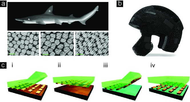
Bumpy protrusions on the surface of the lotus leaf at the small length scales have been shown to endow the leaf with the property of super-hydrophobicity (non-wettability) at the large scales [1]. This non-wetting property is the source of the lotus leaf’s acclaimed self-cleaning ability. Similarly, the periodic, small-scale, wavy undulations on the skin of some sharks are thought to reduce the skin’s frictional drag [2], as shown in Figure 1a. Such intriguing links between small-scale mechanical structures and large-scale physical properties, however, are not limited to biological systems. The small-scale topography of natural surfaces, which is generally stochastic, is often referred to as surface roughness. When separating two contacting surfaces, the surfaces’ roughness is typically thought to reduce the adhesion between them [3, 4, 5, 6]. However, there are cases in which roughness is seen to actually enhance adhesion [7, 8]. Small-scale mechanical design can not just modulate surface properties at the large-scale but, in fact, give rise to completely new phenomenon at the large scales. For example, it was shown by Kesari et al. [9, 8, 10, 11, 12] that small-scale surface topography can give rise to the phenomenon of depth-dependent hysteresis at the large scales.
In engineering sciences, there is currently tremendous interest in creating materials with novel properties, such as materials with negative Poisson’s ratios, through the use of small-scale, intricate lattice-based mechanical designs (e.g., Figure 1b). The recent popularity of 3D printing is, presumably, primarily responsible for galvanizing such interests. The concept of modulating material properties at the large scale through incorporating mechanical designs at the small-scale—in contrast to, say, through the use of chemical or metallurgical treatments—has been of interest, in fact, for the past several decades in the composites and the mathematical homogenization communities [13, 14, 15]. However, the focus in engineering and mathematics has primarily been on modulating bulk material properties, such as elastic stiffnesses and thermal conductivities. Needless to add, surface physical properties, such as adhesion, friction, etc., are no less important than bulk properties, and, as can be gleaned from the examples previously mentioned, small-scale mechanical designs can lead to not just modulation but the emergence of completely new surface properties at the large scale. Therefore, a reason behind the engineering community’s narrow focus could be that the mathematical theories that connect large-scale surface physical properties to small-scale mechanical designs are not as well developed as the ones that connect bulk physical properties to small-scale mechanical designs. In this paper, we focus on the surface property of adhesion and present a mathematical theory that connects the large-scale force needed to peel off a thin elastic film from a rigid substrate to the substrate’s small-scale surface topography.
Adhesion is one of the most important surface physical properties. (See [11, 16, 17] for discussions on this aspect.) Adhesive peeling of a thin film from a substrate is ubiquitous in biological and engineering systems and draws growing attention due to its many applications (e.g., Figure 1c). Despite its long history, the topic of thin film peeling continues to reveal new and interesting phenomena. We review some of the recent studies on this topic in §2.
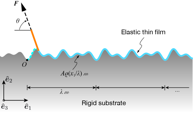
In this paper we study the mechanics of peeling in a plane (2-dimensional) problem. Specifically, we study the peeling of a thin elastic film from a rigid substrate whose surface is nominally flat with superimposed periodic undulations in a single direction. To be more precise, the substrate’s topography is, respectively, invariant and periodic in two orthogonal directions that lie in the substrate’s nominal surface plane. The invariant and periodic directions are shown marked as and , respectively, in Figure 2. The applied tractions as well as all fields in the film also do not vary in the direction. We assume that the film’s de-adherence only takes place at the peeling front, which is a straight line parallel to . We find that in the regime where the substrate’s surface roughness is large, the peel-off force becomes independent of the direction in which the film’s free end is being pulled. This result is in stark contrast to the results from the seminal analysis of Rivlin [18] and Kendall [19], who studied the classical problem of plane peeling of a thin elastic film from a flat surface. In that classical problem the peel-off force strongly depends on the direction of peeling. We also find that this angle-independent peel-off force’s magnitude, in fact, equals the maximum value that is possible for the peel-off force during the plane peeling of a thin elastic film from a rigid substrate, irrespective of the details of the substrate’s profile and the direction of peeling. The aforementioned results are especially significant considering that nowadays it is routinely possible to create highly regular small-scale topographies on engineering surfaces through the use of micro-fabrication and 3D printing technologies.
We make the following assumptions in our problem. We assume that initially the thin film is perfectly adhered to the substrate, i.e., with no gaps between it and the substrate’s surface. Over the adhered region we do not allow for (tangential) slip between the thin film and the substrate’s surface. We model adhesive interactions between the film and the substrate using the JKR theory [20], as per which during peeling the system’s energy increases linearly with the area of the region of the film-substrate interface that comes de-adhered. We consider a force-controlled peeling process. The force is applied to the thin film’s free end and its magnitude and direction can vary in a fairly general way with time, as long as the force is tensile in nature. We term the angle that the applied force makes with the direction that is parallel to and points away from adhered portion of the film the nominal peeling angle, or just the peeling angle for short (Figure 2). We take the peeling process to be quasi-static in nature and ignore all inelastic and inertial effects. We do use the notion of time, however, but only so that we can speak about the sequence of events that take place in our peeling experiment. By a peeling experiment we mean a sequence of peeling angles and force magnitudes applied to the thin film, which are infinitesimally different from each other.
We take the thin film to be composed of a linear elastic material and to be of vanishing thickness. Consequently, we assume that the thin film’s elastic strain energy only depends on its stretching deformations. Specifically, we ignore any “bending energy” in the thin film. The deformations related to stretching, however, can be of finite magnitude. Despite these and the many other assumptions that we introduce over the course of the paper, our analysis reveals important and interesting new mechanics. This is possible, we believe, because we retain the important feature of contact in our problem. That is, we allow for the detached part of the thin film to come into contact with the substrate’s surface and assume that such contact is non-adhesive and frictionless. By retaining this important feature of contact we are able to investigate the regime where the substrate’s surface roughness is large. Additionally, it is in this regime where the peel-off force becomes independent of the peeling angle and the force’s magnitude becomes equal to its maximum value.
The outline of the paper is as follows.
We briefly review some of recent results of the mechanics of peeling in §2. We introduce the technical details of our problem in §3.1. Specifically, we describe the kinematics of our problem in §3.1.1, and present the law that we use for modeling the thin film’s de-adherence in §3.1.2. We take a configuration in our problem to be defined by the de-adhered length, the peeling angle, and the substrate’s surface profile. The de-adhered length is defined in §3.1.1, and is roughly the width of the region on the substrate’s nominal surface in the direction from which the film has been detached. In §3.1.3 we derive the sufficiency condition, which we term the global compatibility condition, for there to be no contact between the detached part of the thin film and the substrate in a given configuration. We present results for the case in which the global compatibility condition holds, i.e., in which there is no contact, in §3.2, and for the case in which it is violated in §3.3. (When the global compatibility condition is violated the configurations that occur during a peeling experiment may or may not involve contact.)
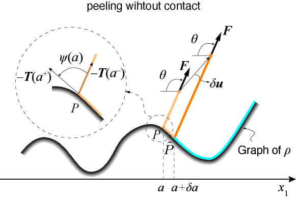
For both cases we give explicit, analytical results for computing the equilibrium force given the true peeling angle, which is the angle at which the detached part of the film leaves the substrate (Figure 3). For the case in which there is no contact, we present explicit results for computing the true peeling angle from the substrate’s profile, and for determining an equilibrium state’s stability just from the substrate’s surface curvature. We call a configuration along with the magnitude of the force acting on it a state. For the case in which there can be contact, we present an algorithm (see Algorithm 1) that allows for numerically calculating the a configuration’s true peeling angle, and determining an equilibrium state’s stability.
For both cases, we also prove that there exist critical force values, such that if the magnitude of the applied force lies outside their range, the film either continuously de-adheres or adheres until the film is completely peeled off from or adhered to the substrate. We term these quantities the peel-initiation and peel-off forces. We determine the peel-initiation force’s minimum value as well the peel-off force’s maximum value for the wide class of surface profiles that we consider in our problem and all admissible peeling angles.
We prove that in a peeling experiment in which the peeling angle is held at a fixed value that is both acute (resp. obtuse) and violates the global compatibility condition the peel-off (resp. peel-initiation) force achieves its maximum (minimum) value, irrespective of the substrate’s profile.
Again considering experiments in which the peeling angle is held constant we show in §4 that as the surface roughness becomes large the peel-off force becomes independent of the experiment’s peeling angle. This happens irrespective of the substrate’s surface profile. The surface roughness becoming large is equivalent to the scenario where the lateral length scales in the substrate’s surface topography becomes small. Furthermore, we also show that the magnitude of that angle-independent, peel-off force equals the maximum that is possible to be achieved.
We conclude the paper by discussing the effect of the thin film’s elastic bending energy on the peel-off force in §5.
2 Literature review
The mechanics of thin film peeling has been extensively studied over the decades after the seminal work of Rivlin [18] and Kendall [19], who analyzed the peeling of a thin film from a flat surface and its importance in understanding the adhesion mechanisms in thin film-substrate systems. For example, Pesika et al. [23] presented a peel-zone model to study the effect of the peeling angle and friction on adhesion based on the microscopic observation of the geometry of the peel zone during film detachment. Chen et al. [24] considered the effect of pre-stretching the film in Kendall’s peeling model and found that the pre-tension significantly increases the peeling force at small peeling angles while decreasing it at large angles. Molinari and Ravichandran [25] proposed a general model for the peeling of non-linearly elastic thin films and investigated the effects of large deformations and pre-stretching. Begley et al. [26] developed a finite deformation analytical model for the peeling of an elastic tape and defined an effective mixed-mode interface toughness to account for frictional sliding between the surfaces in the adhered region. Gialamas et al. [27] used a Dugdale-type cohesive zone to model adhesion between an incompressible neo-Hookean elastic membrane and a flat substrate and carried out both single- and double-sided peeling analysis, while ignoring the membrane’s bending stiffness. Menga et al. [28] investigated the periodic double-sided peeling of an elastic thin film from a deformable layer that is supported by a rigid foundation. Kim and Aravas [29] performed an elasto-plastic analysis of a thin film peeling problem in which the de-adhered part of the film is in pure-bending. Kinloch et al. [30] performed an elasto-plastic analysis of the peeling of flexible laminates and calculated the fracture energy, which included not just the energy required to break the interfacial adhesive bonds but also the energy dissipated in the plastic/viscoelastic zone at the peeling front. Wei and Hutchinson [31] numerically investigated the steady-state, elasto-plastic peeling of a thin film from an elastic substrate using a cohesive zone model. Loukis et al. [32] analyzed the peeling of a viscoelastic thin film from a rigid substrate and related the fracture energy and peel-off force to the peeling speed and film thickness. Afferrante and Carbone [33] investigated the peeling of an elastic thin film from a flat viscoelastic substrate and gave a closed-form expression relating the peeling force to the peeling angle and the work of adhesion.
Spatial heterogeneity in the thin film’s elasticity and the interface’s strength can lead to significant enhancement of the effective peel-off force. The role of spatial heterogeneity in peeling was first highlighted by Kendall [34] who carried out peeling experiments using an elastic thin film that had alternating large and small bending stiffness regions. He varied the stiffness by either introducing reinforcements at select positions on a uniform thin film or by varying the film’s thickness along its length. He peeled the film from a rigid substrate at a constant force and observed abrupt changes in the speed of the peeling front at the boundaries between the stiff and compliant regions, and an overall enhancement in the peeling force. Ghatak et al. [35] and Chung and Chaudhury [36] performed displacement-controlled peeling experiments between a flexible plate and an incision-patterned thin elastic layer and found that the patterns significantly enhanced the effective adhesion. They attributed the enhancement to arrest and re-initiation of the peeling front motion at the edges of the features in the pattern. More recently, Xia et al. [37, 38, 39] experimentally and theoretically investigated the peeling of an elastic thin film while spatially varying the bending stiffness and interface strength in it. They showed that the film’s large-scale (“effective”) adhesive properties could be significantly enhanced through the use of small-scale spatial heterogenity.
There have been several studies that investigate the effect of surface roughness on thin film adhesion. For instance, Zhao et al. [40] simulated the peeling of a hyperelastic thin film from a rough substrate using finite elements and a cohesive zone model. They found that the peeling force could be increased by introducing a hierarchical wavy interface between the film and the substrate. Ghatak [41] theoretically investigated the peeling of a flexible plate from an adhesive layer which was supported on a rigid substrate and had spatially varying surface topography and elastic modulus. He found that the maximum adhesion enhancement took place when the surface height and elastic modulus varied in phase. Peng and Chen [42] studied the peeling of an elastic thin film from a rigid substrate having sinusoidally varying surface topography. They computed the peeling forces for different peeling angles and surface topography parameters and found that the maximum peeling force could be significantly enhanced by increasing the substrate’s surface roughness. To our knowledge there have not been any studies that consider contact between the de-adhered portion of the film and the substrate, or which study the stability of the equilibrium configurations, as we do in this current paper. The surface topography that we consider is fairly general and the regime we explore, namely where the lateral length scales in the substrate’s surface topography are much smaller than the other length scales in the problem, has also not been explored within the context of thin film peeling.
3 Theory of wavy peeling
3.1 Model
3.1.1 Geometry and kinematics
Figure 2 shows the geometry of our wavy peeling problem. Let be a three-dimensional, oriented, Hilbert space, and let the Euclidean point space be ’s principle homogeneous space. The elements of have units of length. The physical objects in our peeling problem are contained in . The origin of , which we denote as , is marked in Figure 2. The vector set , where the index set , is an orthonormal set in . That is, , where ,, the symbol denotes the inner product operator between the elements of , and is the Kronecker-delta symbol, which equals unity if and naught otherwise. A typical point is identified by its coordinates 111In our work the manner in which the information about a physical quantity’s units is stored is different from how that is usually done. We model different physical quantities as vectors belonging to different vector spaces. We store the information about a physical quantity’s units in the basis vectors we choose for that quantity’s vector space. For example, we may take to represent a motion of (or ) in a certain fixed direction in . In that case , as a consequence of its definition, would denote a motion of (resp. ) in the same direction as . Thus, in our work the components of a physical quantity with respect to the basis vectors chosen for its vector space will always be non-dimensional. For example the components of with respect to , namely , are dimensionless. that are defined such that . The vector is called ’s position vector.
Note that the vector set is different from ; it is defined as , where , for , and . The set is an orthogonal, but not an orthonormal, basis for . We will be following the Einstein summation convention in this paper222We follow the Einstein summation convention in this paper. If a symbol has an italicized, light-faced latin character that appears as its subscript/superscript then that subscript/superscript denotes an index and that symbol along with that subscript/superscript denotes a component of a linear mapping. An index that appears only once in a term is called a “free” index. A free index in a term denotes that the term in fact represents the tuple of terms created by varying the free index in the original term over . An index that appears twice in a term is called a “repeated index”. A repeated index in a term denotes a sum of the terms that are created by varying the free index in the original term over ., and write expressions such as and simply as and , respectively, and lists such as , and simply as .
The substrate is a rigid solid whose points’ position vectors belong to the set
| (3.1) |
where , , is a surjective, 1-periodic function, and is the set of real numbers. By 1-periodic we mean that for all . Without loss of generality we take . We also assume that and its first and second derivatives, which we denote as and , respectively, are non-constant, continuous functions, i.e., . We call , , , and the substrate surface’s aspect ratio, amplitude, periodicity, and profile, respectively.
We take the thin film to be of width , of thickness , and to be perfectly adhered to the substrate’s surface in its initial, or reference, configuration. Here and are physical parameters and have units of length. Say the units of and is some length , which, for example, may stand for meters, then we would say that the magnitude of (resp. ) is (resp. ) iff (resp. ). Thus, initially the configuration of the thin film can be described as
| (3.2) |
where 333As is standard in continuum mechanics, we will be referring to a particular thin film material particle using the coordinates of the the spatial point that it occupied in the initial configuration. That is, when we say a material particle , we in fact are referring to the material particle that in the initial configuration occupied the spatial point with coordinates . For the sake of brevity, we will be referring to a material particle simply as , since the second co-ordinate of any spatial point that was occupied by a thin film material particle in the initial configuration is fully determined by the point’s first co-ordinate (cf. (3.2)). Finally, when we say “the (thin-film) material particle ”, where , we in fact mean the group of material particles , where . .
We model the peeling process by assuming that any deformed configuration of the thin film can be described as444In standard continuum mechanics the reference and deformed configurations are taken to belong to different spaces. In contrast, here we take both the reference and deformed configurations, and , to belong to the space space, namely .
| (3.3a) | |||
| where | |||
| (3.3b) | |||
and their derivatives, denoted as and , are continuous. We further assume that for all , for some , and for all . We refer to as the de-adhered length. We call the peeling front and the adhered region.
On knowing the de-adhered length the length of the film peeled from the substrate can be computed as , where is defined by the equation
| (3.4) |
We refer to as the peeled length, and will often abbreviate it as .
3.1.2 Evolution law for de-adherence
In postulating the evolution law for de-adherence, we ignore all dynamic effects, such as inertial forces, kinetic energy, and viscoelastic behavior in the thin film. As we mentioned in §1, we do use the notion of time, but only so that we can speak about the sequence of events that take place in our peeling experiment.
In our peeling experiment the thin film de-adheres due to the application of the force to its free end, which initially is at , the origin of . We think of force as a linear map from into a one dimensional vector space whose elements have units of energy. The set of all forces can, of course, be made into a vector space, which we will denote as . We use the set as a basis for , where are defined such that . The symbol , which appears in the last expression, is defined to be equal to the energy , where is the thin film’s Young’s modulus. We express as , where and . The angle is shown marked in Figure 3. It is prescribed as part of the problem’s definition. We call it the nominal peeling angle, or simply peeling angle for short. We denote the position vector of the free end of the thin film, on which acts, as , and will often refer to this quantity as simply the force-position-vector. Our experiment is force controlled and quasi-static. By force-controlled we mean that while the system’s configuration is changing, is held fixed. If our experiment were a general force controlled experiment, then we would be allowed to vary once the adhered region had stopped evolving. However, in our experiment we are only allowed to vary after the adhered region has stopped evolving. By quasi-static we mean that each variation in is of infinitesimal magnitude and is applied all at once at a particular instance in time.
Consider an experimentally observed configuration of the thin film , in which the de-adhered length is , the peeled length is , the force position vector is , and the force is . Imagine that a force variation of is then abruptly added to the force that was previously acting on the thin film so that the new force is . As a result, the thin film’s configuration will evolve to a new configuration , in which the de-adhered length is , the peeled length is , the force-position-vector is , and, of course, the force is . We postulate that the new configuration is the one that locally minimizes the system’s total potential energy and is closest to .
To make the postulate precise, consider a configuration that is close to and has the same force as , i.e., . The de-adhered and peeled lengths, and the force-position-vector in are, however, different from those in ; we denote them, respectively, as , , and . Since , i.e. the peeled section of the film is in tension, the variations and , in fact, depend on . Thus, these variations are to be interpreted as abbreviations for and , respectively. Let the difference in the system’s potential energy between the configurations and be , where is a constant and has unit of energy, and we refer to as the non-dimensional potential energy variation. In our model of the wavy peeling experiment, we take to be a sum of three different energy variations. These variations take place, respectively, in the energy stored in the interbody adhesive interactions between the thin film and the substrate, the elastic strain energy stored in the peeled part of the thin film, and, finally, the energy stored in the apparatus that maintains the constant force between the configuration and .
We model adhesive interactions between the thin film and the substrate using the JKR theory [20]. According to this theory, the formation of an interface region of area lowers the system’s total potential energy, irrespective of the shape of the interface region or any other details of the experiment, reversibly by . Here, is the Dupré work of adhesion [43, p. 30]. Thus, the variation in the potential energy stored in the interbody adhesive interactions is
| (3.5) |
where is defined such that . That is, is the non-dimensional work of adhesion.
We assume that the peeled part of the film is in uniform, uniaxial tension. It follows from this assumption that the strain in the peeled part of the film is also uniform, and uniaxial, and that its magnitude is equal to . It also follows that the variation in the elastic strain energy stored in the thin film is
| (3.6) |
Usually, the above term is supplemented by an additional term that corresponds to bending energy in the thin film [42]. We, however, ignore the film’s bending energy in our model. As we state in our closing remarks, we believe that ignoring the bending energy is unlikely to significantly affect our estimates for the film’s peel-off force in the type of the peeling experiments that we consider in this paper.
The variation in the potential energy of the apparatus maintaining the constant force is . Say . This variation can therefore be written as
| (3.7) |
where , , and . It follows from the previous discussion that,
| (3.8) |
As is the case with and , the symbol in (3.8) is, in fact, an abbreviation for the value .
Since and depend on , the formula for given by (3.8) needs to be further refined before it can be used for determining whether or not a particular de-adhered length is in equilibrium; and, if is in equilibrium, then for determining the stability of that equilibrium. The particulars of the requisite refinement depend on whether or not the peeled part of the film contacts the substrate. Therefore, we will be making separate refinements of (3.8) for the cases of no-contact and contact in §3.2 and §3.3, respectively. In both cases, however, the refinement process will involve determining the asymptotic dependence of and on as , and then using that information to determine the asymptotic dependence of on .
3.1.3 Conditions for the peeled part of thin film to not contact the substrate
Let be , where is defined in (3.3b). Because a material particle is de-adhered from or adhered to the substrate (depending on whether is less than or greater than ), the vector will often be discontinuous at . However, since we have assumed , , and to be continuous, the following right and left hand limits of as are well defined:
The vector is essentially the tangent to the substrate’s surface profile at , and the vector points in the direction the detached part of the thin film leaves the substrate’s surface at the peeling front. (See Figure 3.) We call the angle between and the true peeling angle . For the thin film to not go through the substrate immediately after de-adhering from it, it is necessary that
| (3.9) |
We refer to (3.9) as the local compatibility condition.
It can be shown that once the local compatibility condition is satisfied, the peeled part of the thin film will not contact the substrate anywhere, irrespective of the location of the peeling front iff
| (3.10a) | ||||
| where | ||||
| (3.10b) | ||||
| (3.10c) | ||||
We refer to (3.10) as the global compatibility condition.
3.2 Peeling with no contact
In this section we study the case in which the local and global compatibility conditions (i.e., (3.9) and (3.10)) are satisfied, and therefore the peeled part of the thin film does not contact the substrate anywhere.
3.2.1 Energy variation
Since the peeled part of the thin film is not in contact with the substrate, it follows that
| (3.11) |
where is the uniform, uni-axial strain in the peeled part of the thin film, and . It follows from (3.4) that
| (3.12) |
where
| (3.13a) | ||||
| (3.13b) | ||||
Substituting the asymptotic expansions for and as into (3.11), and then substituting the resulting asymptotic expansion for into (3.7), we find that
| (3.14) | ||||
The symbol , that appears in (3.14) and elsewhere, is the Bachmann-Landau “Small-Oh” symbol. Its primary property of relevance is that , where , as .
3.2.2 Equilibrium state
Since we take , it follows that and are continuous, and, as a consequence, that is continuous. It then follows that for to be an equilibrium de-adhered length it is necessary that . For a given and there can, however, be more than one de-adhered length that is in equilibrium. We characterize all those lengths by saying that they belong to the set
| (3.19) |
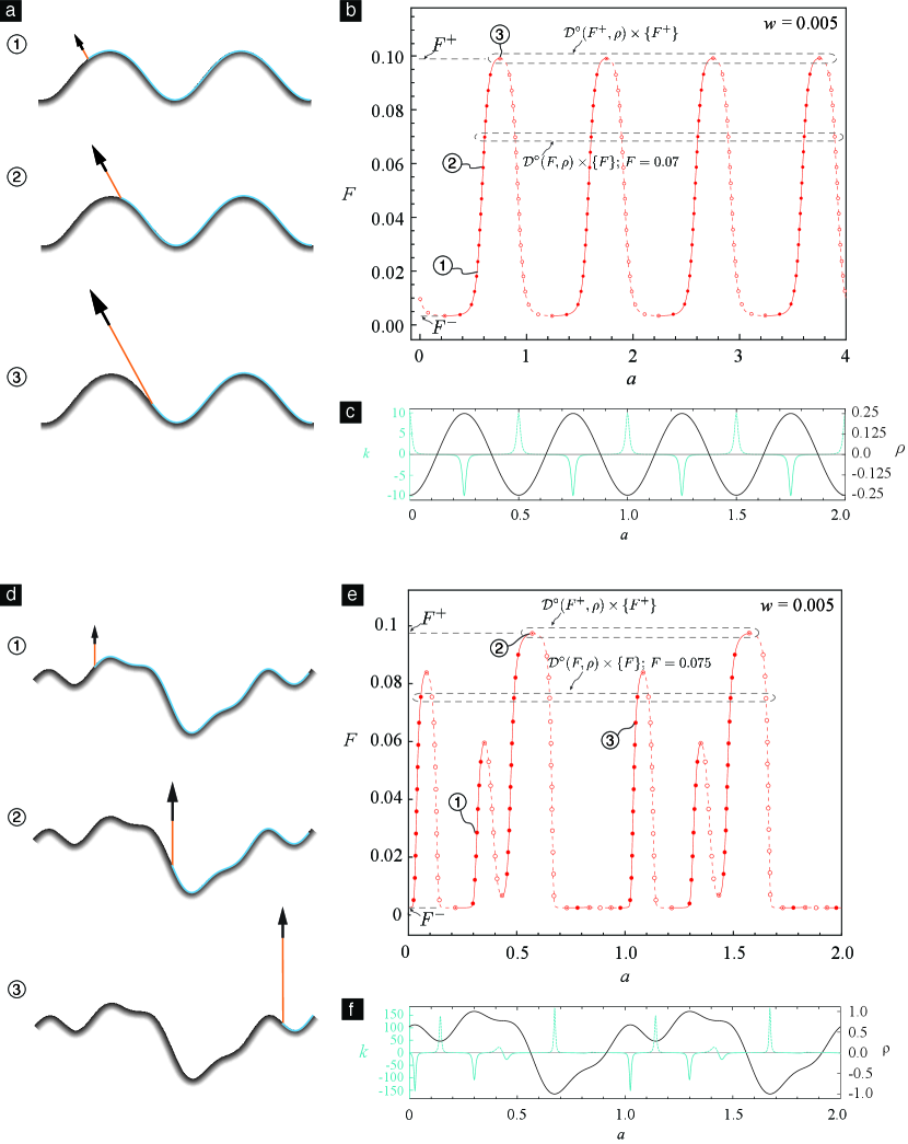
We plot the set of points
for various values, for the example surfaces shown in Figures 4a and c in Figures 4b and d, respectively. As can be seen, the peeling force for peeling on wavy surface is not constant, but varies with the same periodicity of the wavy surfaces. It can be shown that the point set , for any admissible , falls on the graph of the periodic function
| (3.20a) | ||||
| where is defined in (3.15) and is defined by the equation | ||||
| (3.20b) | ||||
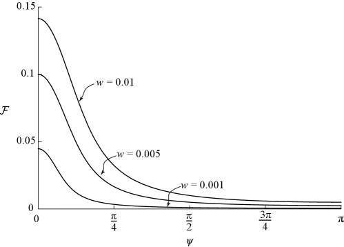
We only consider cases in which the work of adhesion is non-negative. It therefore follows from (3.20b) that is always non-negative. The graph of for different values is shown in Figure 5. As can be seen, is a strictly decreasing function whose value at any admissible increases with .
Kendall analyzed the peeling of a thin film on a flat smooth surface [19]. By setting for a flat surface, which leads to from (3.15), Kendall’s result can be immediately recovered from (3.20) which gives the peeling force as
| (3.21) |
which is a constant for a given nominal peeling angle .
For a general peeling process we define the supremum and infimum equilibrium force values, denoted as and , respectively, as
| (3.22) |
It can be shown that the maximum and minimum values of the function are and , respectively. This implies that is bounded above by and is bounded below by .
We denote the maximum and minimum values of the true peeling angle during peeling as and , respectively. In the current case of peeling with no contact it follows from the fact that is a monotonically decreasing function that
| (3.23a) | ||||
| where | ||||
| (3.23b) | ||||
Since is always non-negative it follows from (3.23a) that .
Theorem 3.1.
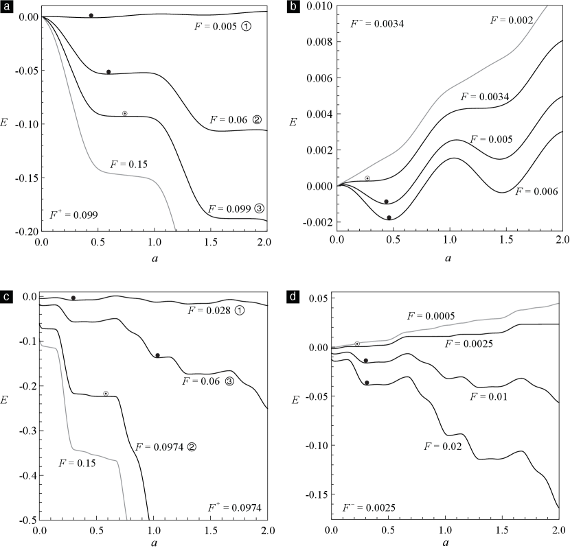
If then there does not exist any equilibrium de-adhered length at that (e.g., see Figures 4b and e).
Proof.
Since are the maximum and minimum values of , respectively, and from (3.9) we have
| (3.24) |
From (3.24) and the fact that the cosine function is strictly decreasing in the interval , we find that
| (3.25) |
The inequalities (3.25) allow us to express as either or ; and, though they depend on , , are always non-negative.
Let us first consider the case . When is strictly greater than it can be represented as for some . Using this representation for and expressing as in (3.18b) we get that
| (3.26) |
Equation (3.4) implies that the derivative of the peeled length is always positive. For that reason and since it follows from (3.26) that when
| (3.27) |
It follows from (3.27) and the facts that and are positive and and are non-negative that when
| (3.28) |
Since for equilibrium it is necessary that it follows from (3.28) that there can exist no equilibrium de-adhered lengths when .
Now consider the case . When it can be represented as for some . Representing this way and expressing as in (3.18b) we determine that
| (3.29) |
Since and it follows from (3.29) that when
which can be re-arranged to read
| (3.30) |
Recalling that is non-negative and is positive it follows from (3.30) that when
| (3.31) |
For the same reason as before, the inequality (3.31) implies that when is less than but still non-negative then there cannot exist any de-adhered lengths that are in equilibrium. ∎
The inequality (3.28) implies that the derivative of the total energy w.r.t will be negative when is greater than irrespective of the value of , , or the nature of (see, e.g., Figures 6a and c). Thus, if the de-adhered length will grow without bound. Realistically, however, the de-adhered length will keep growing until the film completely detaches from the substrate. For that reason we call the peel-off force.
The result that (3.31) holds in the case where implies that the derivative of the total energy with respect to the de-adhered length in that case is positive irrespective of any other details in the problem (see, for example, Figures 6b and d). Therefore, if and the de-adhered length is initially naught, then the de-adhered length will not grow or if it is initially non-zero then it will keep decreasing, i.e., the peel front will keep receding until the entire thin film is adhered to the substrate. For this reason, we call the peel-initiation force.
3.2.3 Stability of equilibrium state
We study the stability of the local equilibria by examining the sign of the second variation of the total potential energy. Specifically, a configuration with the de-adhered length is a stable equilibrium state iff belongs to the set
| (3.32) |
It is a neutral equilibrium state iff belongs to the set
| (3.33) |
and is an unstable equilibrium state if belongs to the set , which is a set of all de-adhered lengths that belong to but not to or .
Stability and surface curvature
Suppose is an equilibrium de-adhered length at the force . Then it is necessary that and satisfy the equation , where on the right hand side is the function defined in (3.20). Upon substituting in (3.18c) with , and then simplifying the resulting equation, we get that
| (3.34) |
where
| (3.35) |
is the signed curvature of the graph of . The mean curvature of the substrate’s surface at the point whose coordinates w.r.t to and are and , respectively, equals . Therefore, we will often refer to as the substrate’s surface curvature.
If , then from (3.20) we have that . Consequently, from (3.34), for all . Therefore, when all states are neutral-equilibrium states. In the following section we take that is positive (recall that ).
If vanishes then it follows from (3.34) that belongs to , i.e., that the corresponding state is a neutral equilibrium state.
It follows from the definitions of , , and and the smoothness of that iff . So, if does not vanish then is different from , which implies from the definitions of , , and that is different from . This last deduction in conjunction with (3.24) implies that when is not naught, is positive. Hence, it follows from (3.34) that the configuration is stable (resp. unstable) when is negative (resp. positive). These results, which connect an equilibrium state’s stability to the surface curvature, are illustrated by Figures 4b–c for a sinusoidal surface and by Figures 4e–f for a complicated surface.
Positive, negative, and zero values of the function imply stable, unstable, and neutral equilibria, respectively
Again, let be an equilibrium de-adhered length at the force . From (3.20) we have that
| (3.36) |
Recall that we deduced that when all configurations are neutral equilibrium configurations. Therefore, in the following two paragraphs we take that .
Say vanishes. It can be checked using (3.13a) that is always positive, and since we have assumed that it can be shown that the expression within the large parenthesis on the right hand side of (3.36) is always positive. Therefore, if vanishes then we have the following three cases from (3.36): (i) the factor vanishes, (ii) the factor vanishes, (iii) both these factors vanish. The factor vanishes in both case (i) and (iii). Let us focus on case (ii). If vanishes then we know from (3.24) that , which then implies, based on the discussion following (3.34), that has to also vanish. then we know from (3.24) that , which then implies, based on the discussion contained in the third paragraph following the one containing (3.34) that, has to also vanish. Thus, vanishes in all three cases. That is, if is equal to zero then is also equal to zero. This last deduction in light of the results presented in Stability and surface curvature implies that if vanishes then the configuration corresponding to is a neutral-equilibrium configuration.
Now say that is positive (resp. negative). As previously stated, since we have assumed that the expression within the large paranthesis on the right hand side of (3.36) is always positive. The factor is positive since we can show using (3.24) that it is always non-negative and if it were to vanish then that would contradict the assumption that is non-zero. This, in conjuction with (3.36), imply that is negative (resp. positive) whenever is positive (resp. negative). In light of the results presented in Stability and surface curvature, this last deduction implies that when is positive (resp. negative) then the corresponding equilibrium configuration is stable (resp. unstable).
3.3 Peeling process that might involve contact
If is kept fixed during the peeling process and that constant violates the global compatibility condition (3.10), then there will exist some configurations during the peeling process that will involve contact777 This, of course, does not mean that in such a peeling process all configurations will involve contact. That is, there can exist configurations that involve no contact during parts of the peeling process (see, e.g., subfigure (b) in Figure 8). . We provide a procedure for determining whether or not a given configuration involves contact in §3.3.2. If the configuration does not involve contact, the results needed to compute the force so that is an equilibrium state and the results needed to determine the stability of are given in §3.2.
When involves contact the primitive conditions that determines whether or not a state is in equilibrium remain the same as before. Specifically, even when a configuration involves contact, the state is an equilibrium state iff the de-adhered length in belongs to the set , which is defined in (3.19). Similarly, it qualifies as a stable, neutral, or unstable state depending on whether the de-adhered length belongs to the sets , , or , respectively. These sets are defined in §3.2.3.
What makes the analysis of the case involving contact more challenging is the calculation of the functions and , which are needed for the construction of the sets , , etc. These functions are defined in (3.18a) in terms of the asymptotic expansion of as . The calculation of ’s asymptotic expansion is challenging due to the presence of the term in (3.8). In the case involving contact the term simplifies to , where is ’s magnitude. This is due to the fact that is always in the same direction as (see Figures 12 and 13) when a configuration involves contact. This remains true irrespective of whether the contact region consists of a single contact patch (e.g., see Figure 7) or several contact patches (e.g., see subfigure (a) in either Figure 12 or 13). Thus, calculation of ’s asymptotic expansion requires the calculations of ’s asymptotic expansion, which in this current case is non-trivial. To elaborate, in the case not involving contact, it is straightforward to determine the asymptotic expansion of , e.g. through the use of (3.11) and (3.12). While now in the case involving contact this exercise is relatively more difficult.
We could not obtain a general, closed-form expression for the asymptotic expansion of when the configuration involved contact. However, in §3.3.3 we present a family of four analytical, but not closed-form, expressions for calculating ’s asymptotic expansion, and from that and , that apply to special categories of contact configurations. We describe these four categories, to whom we henceforth refer to as C.1, C.2, etc., shortly in §3.3.1, but we note here that it will follow from their definitions that any contact configuration can be uniquely placed into in one of them.
From the family of functions given in §3.3.3, which apply to different categories of contact configurations, we found that, interestingly, irrespective of which category a contact configuration belongs to the force needed to make the state an equilibrium state is always , where is defined in (3.20b). However, it follows from the family of functions given in §3.3.3 that ’s category is still relevant for determining the nature of ’s stability.
In summary, our method for simulating a peeling process in which violates the global compatibility condition at some stage of the peeling process is as follows. Let the peeling experiment be defined by prescribing the sequence , where , etc., and the symbols and are the de-adhered length and the nominal peel angle, respectively, in the step of the experiment. We compute , the true peeling angle for the step, using Algorithm 1. We place the configuration into one of the four categories, C.1–4, using and (see §3.3.2 for details). We then compute the force such that the state becomes an equilibrium state as . We determine the nature of ’s stability by computing and constructing the sets , , etc. When the contact configuration belongs to either C.1 or C.2 the Algorithm 1 also provides the value of the parameter , which is the distance between the peeling and contact fronts. So, when belongs to either C.1 or C.2 we use that value in conjunction with (3.40b) to compute . When belongs to C.3 or C.4 we compute the value of using (3.42b) or (3.44b), respectively.
We demonstrate our method by using the same two example surfaces that we previously considered in §3.2. The schematics of these simple and complicated wavy surfaces are shown, e.g., in Figures 4a and d, respectively.
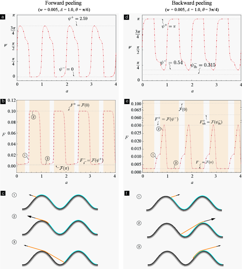
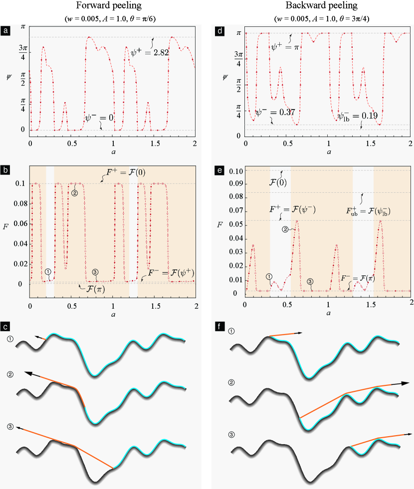
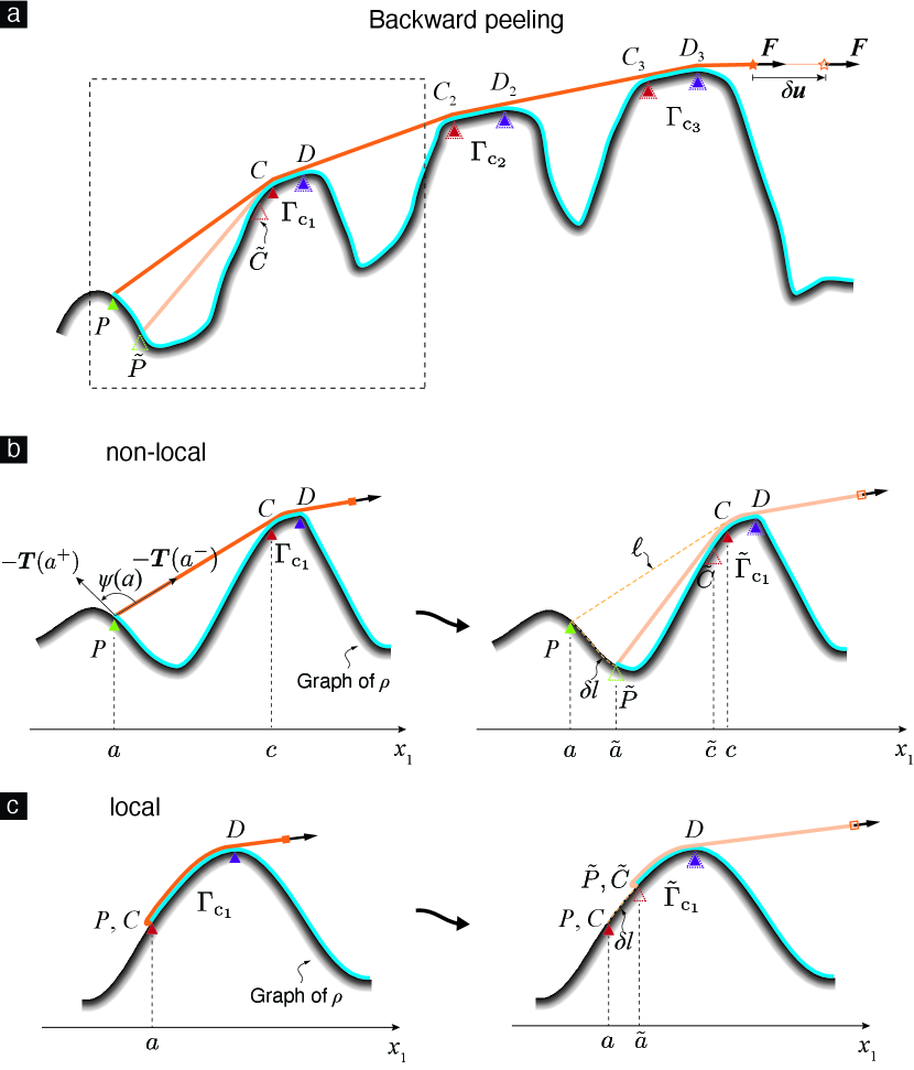
On each surface we simulated two (virtual) peeling experiments. In the first experiment—forward peeling (defined in §3.3.1)—the peeling angle was kept fixed at a value of through out the experiment, while in the second one—backward peeling (defined in §3.3.1)—it was kept fixed at . The constant nominal peeling angles we chose, namely and , violated the global compatibility condition on both our example surfaces. Therefore, the results from §3.2 cannot be used to simulate these experiments, for instance to generate the set
| (3.37) |
for these experiments. Note that a typical point in (3.37) represents an equilibrium state, with its abscissa denoting the state’s de-adhered length and its ordinate the state’s force. Therefore, we applied our method, which we introduced earlier in this section, to the sequence () and computed the sequence , where is the equilibrium force corresponding to ; And constructed (a subset of) (3.37), alternately, as . The sets (3.37) that we generated this way for the forward and backward peeling cases are shown in subfigures (b) and (e), respectively, of Figure 8 for the simple wavy surface and in Figure 9 for the complicated wavy surface.
Note that our method also determines the stability of an equilibrium state and informs us whether or not that state involves contact. In the subfigures (b) and (e) of Figures 8 and 9 the stable equilibrium states are denoted using solid/filled symbols while unstable states are denoted using hollow/unfilled symbols. In the subfigures we identify the states that involve contact by placing them over a yellow background. As can be noted from the subfigure, a yellow region is preceded and followed by white regions, and vice versa. Thus, when the global compatibility condition is violated a sequence of configurations involving contact can be followed by a sequence of configurations not involving contact, and so on.
Finally, our method also provides the true peeling angle sequences in the experiments. These are shown in subfigures (a) and (b) of Figures 8 and 9.
A few representative configurations from the peeling experiments are explicitly sketched in subfigures (c) and (f) of Figures 8 and 9.
3.3.1 The four categories of contact configurations
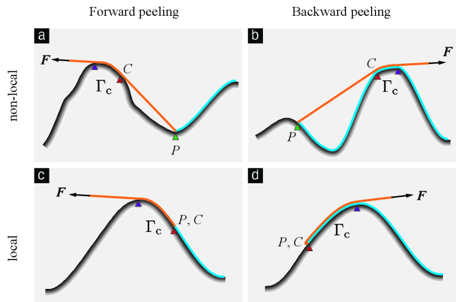
A configuration involving contact can be placed into one of the following four categories.
-
C.1
Forward-peeling, non-local contact (Figure 7a),
-
C.2
Backward-peeling, non-local contact (Figure 7b),
-
C.3
Forward-peeling, local contact (Figure 7c), and
-
C.4
Backward-peeling, local contact (Figure 7d).
We call a configuration a forward-peeling configuration if the in it is less than , and a backward-peeling configuration otherwise. Roughly speaking, we consider configurations of the type shown in Figures 7a and b as those that involve non-local contact, and configurations of the type shown in Figures 7c and d as those that involve local contact. We define local and non-local contact precisely by introducing the notions of contact region and contact front, which we discuss next.
We define the contact region corresponding to the deformed configuration as , where
| (3.38) |
is the substrate’s surface (cf. (3.1)) and is defined in (3.3b). Let be the point in that is closest to in ’s topology; recall here that is the adhered region corresponding to the configuration . We define the contact front as .
We say that a deformed configuration involves local contact iff and involves non-local contact otherwise.
3.3.2 Procedure for determining a configuration’s type—contact or non-contact—and a contact configuration’s category
When satisfies the global compatibility condition then we know that the configuration will be of non-contact type. When the global compatibility condition is violated, as we describe in the next few paragraphs, determining whether or not involves contact, i.e., determining its type, and if it involves contact then determining the contact category that belongs to essentially comes down to determining the true peeling angle .
The true peeling angle is defined in §3.1.3. When satisfies the global compatibility condition is given by (3.15). When violates the the global compatibility condition it can be computed using the numerical procedure that we present in Algorithm 1.
Given a configuration , if the true peeling angle in it is different from (3.15) then is a contact type configuration. Otherwise, it is a non-contact type configuration.
For placing a contact type configuration into one of the four categories described in §3.3.1 it is sufficient to know whether is a forward or backward peeling configuration and whether the contact in it is of the local or the non-local type.
The configuration is a forward peeling configuration if , and a backward peeling configuration otherwise. A contact configuration involves non-local or local contact depending on whether the true peeling angle in it, , lies in the interior or on the boundary of the set .
3.3.3 Asymptotic expansion of and the functions and for the different categories of contact configurations
Categories C.1–2
In §A we show that for these categories
| (3.39) | ||||
where is the distance between and . Recall that and denote the peeling and contact front, respectively (e.g., see Figure 7). We introduced these notions in §3.1.1 and §3.3.1. Substituting the appearing in (3.8) with the expression appearing on the right hand side of (3.39) and then comparing the resulting equation with (3.18a) we get that
| (3.40a) | ||||
| (3.40b) | ||||
Categories C.3
Categories C.4
As can be noted from Figure 13c for this category, . With (3.12) we have
| (3.43) |
It follows from (3.43), (3.8), and (3.18a) that
| (3.44a) | ||||
| (3.44b) | ||||
3.3.4 Remarks on peeling with contact
The results for peeling involving contact shown in Figures 8 and 9 only apply to the sample surfaces shown in Figures 4a and d, respectively. That is, we do not have a general, closed-form, analytical theory for the case in which at least some configurations involve contact. However, we can make the following general, interesting, remarks with regard to the case involving contact.
Theorem 3.2.
During forward peeling when the global compatibility condition (3.10) is violated, specifically when , the peel-off force achieves its upper bound, which is .
Proof.
Consider the configuration in which the de-adhered length . The length is defined in (3.10c). Using Algorithm 1 we show that the true peeling angle in this configuration, , is naught.
We start by showing that the configuration involves contact. Let us assume that the configuration does not involve contact. It then follows from Algorithm 1, line 4 that for all . Recalling ’s definition this last implication can be written more explicitly as
| (3.45) |
for all . Taking the limit in (3.45) and noting that is a continuous function we get that
| (3.46) |
Since , the left hand side in (3.46) simplifies to . It follows from our hypothesis that the global compatibility condition is violated that the right hand side of (3.46) is greater than . Thus, we get a contradiction. Hence, our assumption that the configuration does not involve contact is false.
Since the configuration involves contact we need to move to line 7 of Algorithm 1 for determining the configuration’s true peeling angle. Noting that we have assumed to be a continuous function and, from (3.10b), that is ’s minimum value we get that . This last result together with (3.13a) and (3.35) implies that . The function ’s property that it is a surjective function with the range implies that is negative. As a consequence of these last two implications we need to move to line 8 from line 7 in the algorithm. Since in forward peeling we get from line 8 that the true peeling angle in the configuration is naught, i.e., .
In §3.3 we discussed that the equilibrium force corresponding to a configuration with de-adhered length is . Thus, we the configuration’s equilibrium force is , which simplifies to .
Recall that is the function ’s maximum value. This fact in conjunction with ’s definition (3.22) and the final result from the previous paragraph imply that . ∎
Theorem 3.3.
During backward peeling when the global compatibility condition (3.10) is violated, specifically when , the peel-initiation force achieves its lower bound, which is .
We omit our proof for Theorem 3.3. Since it is quite similar to the one we provided for Theorem 3.2, except that in it we focus on the configuration with de-adhered length instead of the configuration with de-adhered length .
Theorem 3.4.
During backward peeling when the global compatibility condition is violated, specifically when
| (3.47a) | ||||
| the equilibrium force is always less than or equal to , where | ||||
| (3.47b) | ||||
Proof.
In §3.3 we discovered that during backward peeling when the global compatibility condition is violated there will exist some configurations that involve contact and others that do not (see Figures 8e and 9e.)
When a configuration involves contact the true peeling angle is given by (3.15). Since, by hypothesis, and, since by definition, it follows from (3.15) that during backward peeling when the configuration does not involve contact the true peeling angle is greater than , which is nothing but .
When a configuration involves contact then it follows from Algorithm 1 that the true peeling angle is either equal to (local contact) or to (non-local contact), where recall that and are the abscissae of the peeling and contact fronts, respectively. Since we have assumed to be a non-constant function it follows that and hence that . It follows from the definitions of , , and the monotonicity of that . Thus, in the case of contact the true peeling angle is greater than or equal to .
The deductions in the last two paragraphs can be summarized by saying that when (3.47a) holds the true peeling angle is always greater than or equal to . In §3.3 we discussed that the equilibrium force corresponding to the true peeling angle is always , irrespective of whether or not the configuration involves contact. Since is a monotonically decreasing function the last two statements imply that under (3.47a) the equilibrium peeling force is always less than or equal to . ∎
4 Angle-independent optimal peel-off force
In this section, we analyze the asymptotic value of the peel-off force when the substrate’s aspect ratio , or its root-mean-square (RMS)999The RMS roughness of the substrate’s surface is equal to . roughness, becomes large. This is equivalent to, e.g., the case where the substrate’s surface’s periodicity becomes vanishingly small in comparison to its amplitude .
It follows from Algorithm 1 that as becomes large all configurations become contact configurations, irrespective of or , if is different from ; and if none of the configurations involve contact.
When , since none of the configurations involve contact, we can use the results given in §3.2. Specifically, using (3.23b) we get that as becomes large becomes vanishingly small, since in that limit tends to negative infinity. Taking the limit in (3.23a) we get the result that approaches its upper bound as becomes large. This result is shown illustrated in Figure 10.
When , the condition will inevitably get violated for a large enough . Thus, from Theorem 3.2 we get that will eventually equal its upper bound of as becomes large.
When , let us choose an for which is negative. Now consider a sequence of configurations that all have that same , , and but increasingly larger values of . It follows from Algorithm 1 that when becomes large enough all subsequent configurations will be of the non-local-contact type, and that the true peeling angle in all of them can be computed as . Recall that is the contact front’s abscissa. We would expect to vary between the configurations. However, it can be shown, again using Algorithm 1, that once the configurations become of the non-local-contact type the in them also remains fixed, and furthermore that the value of at that is positive. Since and is negative at and positive at as becomes large and tend to , respectively, and, consequently, the true peeling angles tend to naught. Recall from the discussion in §3.3 that irrespective of whether or not a configuration involves contact, the equilibrium force in that configuration can always be computed as , where is the configuration’s true peeling angle. Thus, as becomes large the equilibrium force in the sequence converges to . From (3.22) we know that the peel-off force for each geometry corresponding to a configuration in the sequence, namely that defined by the profile and the peeling angle , is greater than or equal to that configuration’s equilibrium force. As we noted in the discussion immediately ensuing (3.22) the peel-off force, irrespective of profile or peeling-angle, is bounded above by . It follows from the last three statements that for any fixed and as becomes large the peel-off force tends to its upper bound .
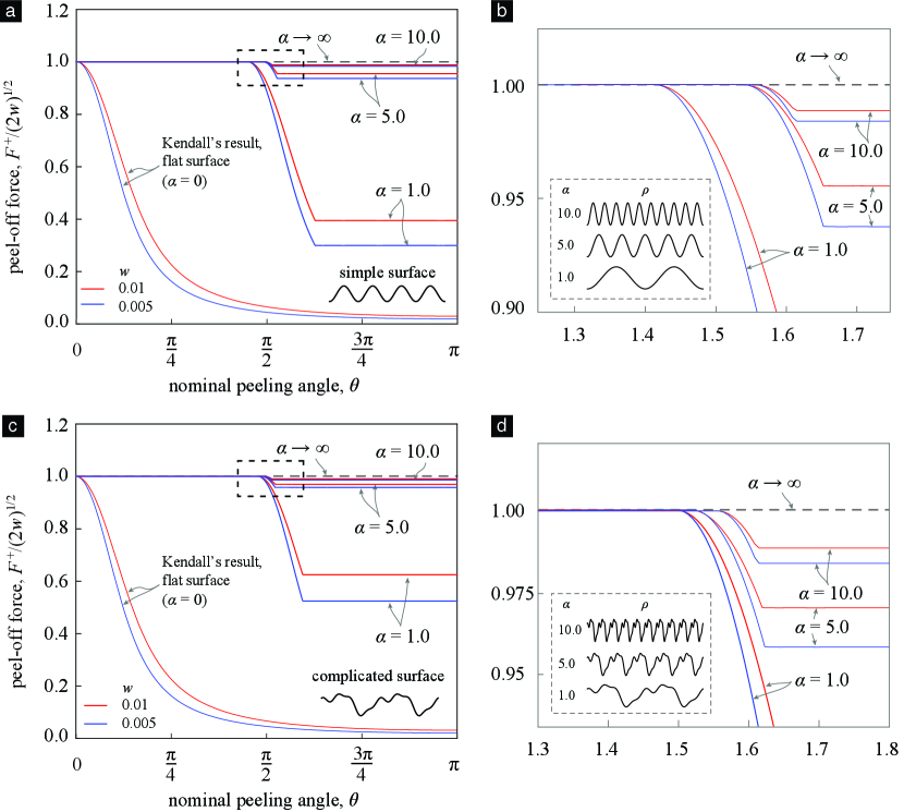
In summary, from the previous three paragraphs we have the important conclusion that as the surface roughness, , is increased the peel-off force tends to its upper bound . This happens independent of the surface’s shape, , and the peeling angle, . We call this phenomenon angle-independent optimal adhesion. This phenomenon is quite interesting considering that adhesion on a flat surface is highly dependent on the peeling angle, and the optimal adhesion is only attained at a single peeling angle, namely for .
We numerically computed the peel-off force for the simple and complicated wavy surface shapes, which we first considered in §3.2, for various peeling angles. For each surface shape and peeling angle we calculated for a sequence of geometries of increasing values. The results of our calculations are shown in Figure 10. As can be seen, at small values, for instance and , the peel-off force depends strongly on . However, as increases the dependence of on becomes weak, such that at large values, e.g. , the calculated peel-off forces appear to be essentially independent of the peeling angle. Finally, irrespective of the peeling angle or the surface shape, the calculated peel-off force values appears to approach from below as increases.
5 Concluding remarks
We conclude this paper by briefly commenting on the effect of bending strain energy on the peel-off force.
Peng and Chen [42] investigated the peeling of an elastic film on a sinusoidal surface. Their sinusoidal surface is the same our simple wavy surface that we first considered in §3.2, and is shown illustrated in Figure 4a. In their analysis they took into account the film’s bending energy, where as in our model we only consider the strain energy due to tension and ignore the strain energy due to bending. They do not consider contact between the thin-film and the substrate in their analysis. Therefore, some insight into the effect of the bending strain energy can be garnered by comparing their analysis to the results that we present in §3.2 (peeling with no contact) when they are particularized to the case of simple wavy surface.
In Peng and Chen’s model the equilibrium peeling force, , is related to the de-adhered length, , as
| (5.1) |
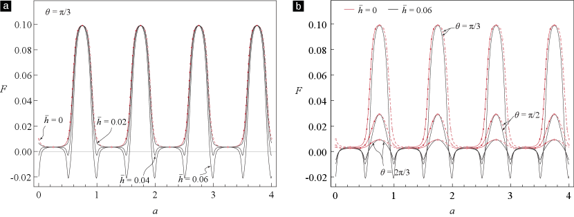
where . On particularizing the results in §3.2 to the case of simple wavy surface our model predicts the same relation between the equilibrium force and de-adhered length as (5.1) except that in it there are no terms containing . That is, in our model’s prediction the third terms from the left within the parenthesis of (5.1), containing , is absent. Since the third term scales with as , Peng and Chen’s results converge to our results as . This fact can also be noted from Figure 11, in which we compare the predictions from Peng and Chen’s model with those from our model for the case of no-contact and peeling on a simple wavy surface for various (in subfigure a) and (in subfigure (b)) values. Even though the above comparison is only for a particular substrate profile, namely the simple wavy surface, we believe that it is reasonable to expect that the effect of the bending strain energy on the equilibrium forces will decrease with decreasing film thicknesses.
Another interesting feature of the above above comaparision that is revealed by the Figure 11 and merits further investigation is that ignoring the bending strain energy seems to have no affect on the peel-off force. The peel-off force which we might recall is the supremum of all equilibrium forces on a given substrate profile and peeling angle. Specifically, as per Figure 11 the surpremum of the equilibrium forces predicted by our’s as well as Peng and Chen’s model appear to be the same. This numerical evidence prompts us conjecture that the bending strain energy, or the film thickness, will have no effect on a film’s peel-off force irrespective of the substrate profile or peeling angle.
Acknowledgment
The authors gratefully acknowledge support from the Office of Naval Research (Dr. Timothy Bentley) [Panther Program, grant number N000141812494] and the National Science Foundation [Mechanics of Materials and Structures Program, grant number 1562656]. Weilin Deng is partially supported by a graduate fellowship from the China Scholarship Council.
Appendix A Derivation of for peeling involving contact
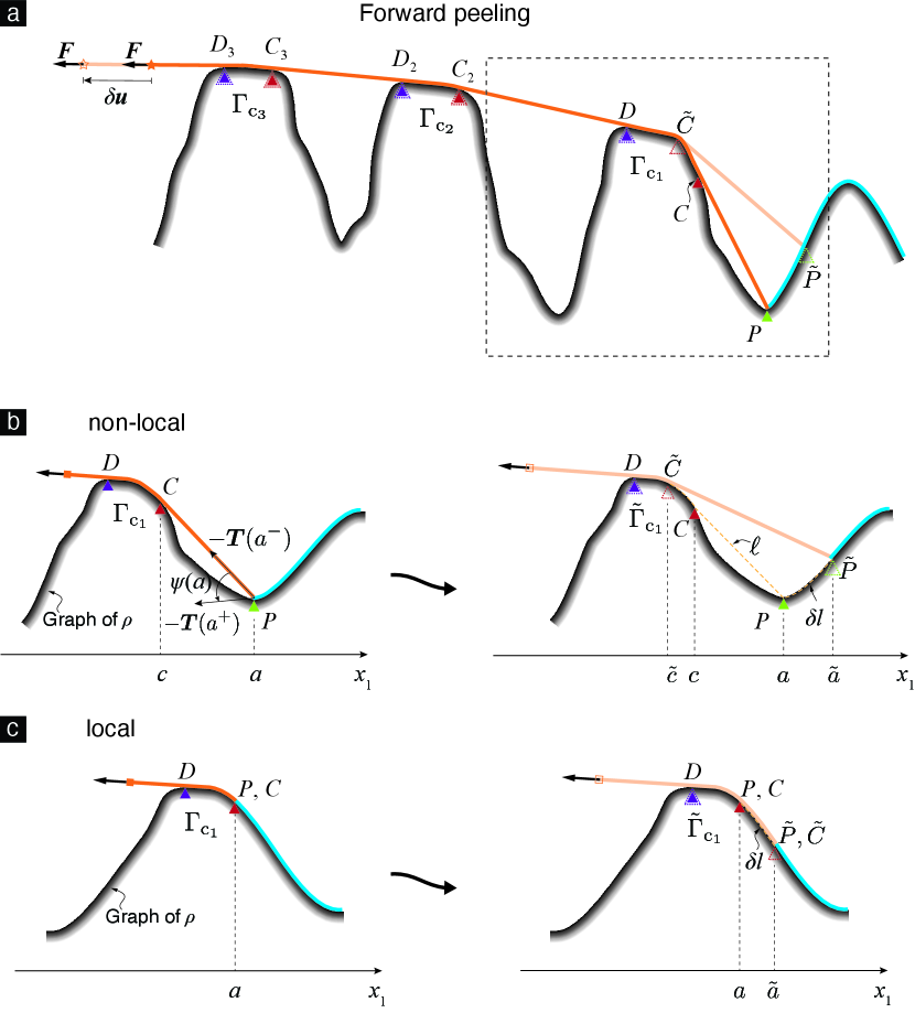
Configurations that involve contact during a generic forward peeling experiment are shown in Figure 12, and similar configurations from a backward peeling experiment are shown in Figure 13. For concreteness we focus on the forward peeling experiment, however, our remarks apply to the backward peeling experiment as well. The peeled part and the remainder of the adhered part of the thin film in the configuration are shown, respectively, in dark orange and blue in Figure 12a. We perturb slightly to obtain the nearby configuration . The peeled part of the thin film in is shown in light orange in Figure 12a. Recall that and denote the peeling and contact fronts in . We denote the peeling and contact fronts in as and .
The quantity that we aim to compute, namely, , is related to the thin film’s kinematics. The thin film’s kinematics take place in . However, since the thin film’s kinematics do not vary in the direction, can be computed by only analyzing the kinematics that take place in, say, ’s - plane. Therefore, we will be focusing all our analysis related to computing only to ’s - plane. In order to avoid the introduction of more symbols, we will use the same symbols that we introduced to refer to subsets of to refer to the quantities that result from the projection of those subsets into the - plane. For instance. The peeling and contact fronts, and , are line segments in . However, we will be denoting their projections into the – plane, which are points in , also as and , and refer to them as the peeling and contact point, respectively. Similarly, we denote the peeling and contact points in as and .
We consider a general contact scenario in which the contact region consists of several disjoint contact patches, ,, etc. In Figure 12a we mark the regions on the substrate which mate with these contact patches in as , ,…, . We call the first contact region, and the last contact region. By definition, the point on the substrate where the first contact region begins is the contact point . We mark the point where the first contact region ends as . Similarly, we mark the points where the , , contact region begins and ends as and , respectively. We denote the location of the thin film’s terminal end in as .
As we perturb the thin film’s configuration from to , the peeling front moves from to , the contact front moves from to , and the terminal end from to . Interestingly, however, none of the other features that define the thin film’s geometry move during this perturbation. Specifically, in the first contact region still ends at , and all the other contact regions still begin and end at the same points that they did in .
The length of the peeled part of the film in can be computed as the sum of the lengths of the line segment , the arc ¿ , the line segment , the arcs ¿ , , and the line segments , , and, finally, the line segment . Based on the discussion in the previous paragraph, the length of the peeled part in is equal to the sum of the lengths of the line segment , the arc ¿ , and, as before, the line segment , the arcs ¿ , and the line segments , and, finally, the line segment . The difference in the length of the peeled part between and , therefore, is
The length difference can, alternately, also be computed as . Equating these two expressions for the length difference and noting that is in fact we get that
| (A.1) |
The term in (A.1) can be computed as
| (A.2) |
where the plus sign is for the case of forward peeling, while the minus sign is for the case of backward peeling.
The points , , , and are shown marked in, e.g., Figure 12a. From the definitions of peeling and contact fronts it follows that the coordinates of the points and are, respectively, and . By denoting the abscissa of the points and as and it follows for similar reasons that these points’ coordinates are and , respectively. The line segments and are tangent to the graph of at and , respectively. (These aspects of the film’s geometry are especially clear in Figure 12b.) Using this information it can be shown that
| (A.3a) | ||||
| (A.3b) | ||||
Using the knowledge of , , , and ’s coordinates, and (A.3) it can be shown that
| (A.4) | ||||
| (A.5) |
Substituting , , and in (A.1) with the right hand sides of (A.2), (A.4), and (A.5), respectively; then writing as , and as the right hand side of (A.9) in the resulting equation; and then, finally, expanding the resulting equation in series of , we get that as
| (A.6) | ||||
where is an alias for . We introduce this new symbol so as to make some of the results that derive from (A.6) appear more compact. The result (A.6) applies to both forward as well as backward peeling. In arriving at (A.6) we used (3.13), and the result that
| (A.7) |
where the plus sign is for the case of forward peeling, while the minus sign is for the case of backward peeling. The result (A.7) follows from Algorithm 1.
A.1 The asymptotic behavior of as
Expressing as and as , where is some real valued analytic function over , in (A.3b), and then expanding both sides of the resulting equation in series of , we get that as
| (A.8) |
In arriving at (A.8) we made use of the identity that , which is a consequence of the requirement that as . It follows from (A.3a) and (A.8) that
| (A.9) |
References
- [1] Wilhelm Barthlott and Christoph Neinhuis. Purity of the sacred lotus, or escape from contamination in biological surfaces. Planta, 202(1):1–8, 1997.
- [2] Li Wen, James C Weaver, and George V Lauder. Biomimetic shark skin: design, fabrication and hydrodynamic function. Journal of Experimental Biology, 217(10):1656–1666, 2014.
- [3] KNG Fuller and David Tabor. The effect of surface roughness on the adhesion of elastic solids. Proceedings of the Royal Society of London. A. Mathematical and Physical Sciences, 345(1642):327–342, 1975.
- [4] John M Levins and T Kyle Vanderlick. Impact of roughness on the deformation and adhesion of a rough metal and smooth mica in contact. The Journal of Physical Chemistry, 99(14):5067–5076, 1995.
- [5] RA Quon, RF Knarr, and TK Vanderlick. Measurement of the deformation and adhesion of rough solids in contact. The Journal of Physical Chemistry B, 103(25):5320–5327, 1999.
- [6] Yakov I Rabinovich, Joshua J Adler, Ali Ata, Rajiv K Singh, and Brij M Moudgil. Adhesion between nanoscale rough surfaces: Ii. measurement and comparison with theory. Journal of Colloid and Interface Science, 232(1):17–24, 2000.
- [7] GAD Briggs and BJ Briscoe. The effect of surface topography on the adhesion of elastic solids. Journal of Physics D: Applied Physics, 10(18):2453, 1977.
- [8] Haneesh Kesari, Joseph C Doll, Beth L Pruitt, Wei Cai, and Adrian J Lew. Role of surface roughness in hysteresis during adhesive elastic contact. Philosophical Magazine & Philosophical Magazine Letters, 90(12):891–902, 2010.
- [9] Haneesh Kesari and Adrian J Lew. Effective macroscopic adhesive contact behavior induced by small surface roughness. Journal of the Mechanics and Physics of Solids, 59(12):2488–2510, 2011.
- [10] Weilin Deng and Haneesh Kesari. Depth-dependent hysteresis in adhesive elastic contacts at large surface roughness. Scientific Reports, 9(1):1639, 2019.
- [11] Weilin Deng and Haneesh Kesari. Effect of machine stiffness on interpreting contact force–indentation depth curves in adhesive elastic contact experiments. Journal of the Mechanics and Physics of Solids, 131:404–423, 2019.
- [12] Weilin Deng and Haneesh Kesari. Molecular statics study of depth-dependent hysteresis in nano-scale adhesive elastic contacts. Modelling and Simulation in Materials Science and Engineering, 25(5):055002, 2017.
- [13] Jean-Claude Michel, Hervé Moulinec, and P Suquet. Effective properties of composite materials with periodic microstructure: a computational approach. Computer methods in applied mechanics and engineering, 172(1-4):109–143, 1999.
- [14] Jerry L Ericksen, David Kinderlehrer, Robert Kohn, and J-L Lions. Homogenization and effective moduli of materials and media, volume 1. Springer Science & Business Media, 2012.
- [15] Pedro Ponte Castaneda. Second-order homogenization estimates for nonlinear composites incorporating field fluctuations: I–theory. Journal of the Mechanics and Physics of Solids, 50(4):737–757, 2002.
- [16] Valentin L Popov, Roman Pohrt, and Qiang Li. Strength of adhesive contacts: Influence of contact geometry and material gradients. Friction, 5(3):308–325, 2017.
- [17] Michele Ciavarella, J Joe, Antonio Papangelo, and JR Barber. The role of adhesion in contact mechanics. Journal of the Royal Society Interface, 16(151):20180738, 2019.
- [18] R.S. Rivlin. The effective work of adhesion. Paint Technol., 9:215–218, 1944.
- [19] K. Kendall. Thin-film peeling-the elastic term. Journal of Physics D: Applied Physics, 8(13):1449, 1975.
- [20] KL Johnson, K Kendall, and AD Roberts. Surface energy and the contact of elastic solids. Proceedings of the Royal Society of London A: Mathematical, Physical and Engineering Sciences, 324(1558):301–313, 1971.
- [21] 3d printed helmet.
- [22] Xue Feng, Matthew A Meitl, Audrey M Bowen, Yonggang Huang, Ralph G Nuzzo, and John A Rogers. Competing fracture in kinetically controlled transfer printing. Langmuir, 23(25):12555–12560, 2007.
- [23] Noshir S Pesika, Yu Tian, Boxin Zhao, Kenny Rosenberg, Hongbo Zeng, Patricia McGuiggan, Kellar Autumn, and Jacob N Israelachvili. Peel-zone model of tape peeling based on the gecko adhesive system. The Journal of Adhesion, 83(4):383–401, 2007.
- [24] Bin Chen, Peidong Wu, and Huajian Gao. Pre-tension generates strongly reversible adhesion of a spatula pad on substrate. Journal of The Royal Society Interface, 6(35):529–537, 2008.
- [25] Alain Molinari and Guruswami Ravichandran. Peeling of elastic tapes: effects of large deformations, pre-straining, and of a peel-zone model. The Journal of Adhesion, 84(12):961–995, 2008.
- [26] Matthew R Begley, Rachel R Collino, Jacob N Israelachvili, and Robert M McMeeking. Peeling of a tape with large deformations and frictional sliding. Journal of the Mechanics and Physics of Solids, 61(5):1265–1279, 2013.
- [27] Panayiotis Gialamas, Benjamin Völker, Rachel R Collino, Matthew R Begley, and Robert M McMeeking. Peeling of an elastic membrane tape adhered to a substrate by a uniform cohesive traction. International Journal of Solids and Structures, 51(18):3003–3011, 2014.
- [28] N. Menga, L. Afferrante, NM Pugno, and G. Carbone. The multiple v-shaped double peeling of elastic thin films from elastic soft substrates. Journal of the Mechanics and Physics of Solids, 113:56–64, 2018.
- [29] Kyung-Suk Kim and Junglhl Kim. Elasto-plastic analysis of the peel test for thin film adhesion. Journal of Engineering Materials and Technology, 110(3):266–273, 1988.
- [30] A.J. Kinloch, C.C. Lau, and J.G. Williams. The peeling of flexible laminates. International Journal of Fracture, 66(1):45–70, 1994.
- [31] Yueguang Wei and John W. Hutchinson. Interface strength, work of adhesion and plasticity in the peel test. International Journal of Fracture, 93(1):315–333, 1998.
- [32] M.J. Loukis and N. Aravas. The effects of viscoelasticity in the peeling of polymeric films. The Journal of Adhesion, 35(1):7–22, 1991.
- [33] L. Afferrante and G. Carbone. The ultratough peeling of elastic tapes from viscoelastic substrates. Journal of the Mechanics and Physics of Solids, 96:223–234, 2016.
- [34] K. Kendall. Control of cracks by interfaces in composites. Proceedings of the Royal Society of London A: Mathematical, Physical and Engineering Sciences, 341(1627):409–428, 1975.
- [35] Animangsu Ghatak, L Mahadevan, Jun Young Chung, Manoj K Chaudhury, and Vijay Shenoy. Peeling from a biomimetically patterned thin elastic film. Proceedings of the Royal Society of London A: Mathematical, Physical and Engineering Sciences, 460(2049):2725–2735, 2004.
- [36] Jun Young Chung and Manoj K Chaudhury. Roles of discontinuities in bio-inspired adhesive pads. Journal of the Royal Society Interface, 2(2):55–61, 2005.
- [37] Shuman Xia, Laurent Ponson, Guruswami Ravichandran, and Kaushik Bhattacharya. Toughening and asymmetry in peeling of heterogeneous adhesives. Physical Review Letters, 108(19):196101, 2012.
- [38] S.M. Xia, L. Ponson, G. Ravichandran, and K. Bhattacharya. Adhesion of heterogeneous thin films-I: Elastic heterogeneity. Journal of the Mechanics and Physics of Solids, 61(3):838–851, 2013.
- [39] SM Xia, Laurent Ponson, Guruswami Ravichandran, and Kaushik Bhattacharya. Adhesion of heterogeneous thin films ii: Adhesive heterogeneity. Journal of the Mechanics and Physics of Solids, 83:88–103, 2015.
- [40] Hong-Ping Zhao, Yecheng Wang, Bing-Wei Li, and Xi-Qiao Feng. Improvement of the peeling strength of thin films by a bioinspired hierarchical interface. International Journal of Applied Mechanics, 5(02):1350012, 2013.
- [41] Animangsu Ghatak. Peeling off an adhesive layer with spatially varying topography and shear modulus. Physical Review E, 89(3):032407, 2014.
- [42] Zhilong Peng and Shaohua Chen. Peeling behavior of a thin-film on a corrugated surface. International Journal of Solids and Structures, 60:60–65, 2015.
- [43] D. Maugis. Contact adhesion and rupture of elastic solids. Solid State Sciences. Springer, 2000.