∎

¹¹institutetext: Jiachen Jin ²²institutetext: [email protected] ³³institutetext: Hongxia Wang, Corresponding author ⁴⁴institutetext: [email protected] ⁵⁵institutetext: Kangkang Deng ⁶⁶institutetext: [email protected]

College of Science, National University of Defense Technology, Changsha, 410073, Hunan, China.

Anderson acceleration of derivative-free projection methods for constrained monotone nonlinear equations

Jiachen Jin Hongxia Wang Kangkang Deng

(Received: date / Accepted: date)

Abstract

The derivative-free projection method (DFPM) is an efficient algorithm for solving monotone nonlinear equations. As problems grow larger, there is a strong demand for speeding up the convergence of DFPM. This paper considers the application of Anderson acceleration (AA) to DFPM for constrained monotone nonlinear equations. By employing a nonstationary relaxation parameter and interleaving with slight modifications in each iteration, a globally convergent variant of AA for DFPM named as AA-DFPM is proposed. Further, the linear convergence rate is proved under some mild assumptions. Experiments on both mathematical examples and a real-world application show encouraging results of AA-DFPM and confirm the suitability of AA for accelerating DFPM in solving optimization problems.

Keywords:

Anderson acceleration Derivative-free projection method Monotone nonlinear equations Convergence

MSC:

65K05 90C56 68U10

1 Introduction

In this paper, we focus on solving the following monotone nonlinear equations with convex constraint:

F(x)=0,\ x\in\mathcal{C},

(1)

where $F:\mathbb{R}^{n}\to\mathbb{R}^{n}$ is a continuous and monotone mapping, and $\mathcal{C}\subset\mathbb{R}^{n}$ is a closed convex set. The monotonicity of the mapping $F$ means that

(F(x)-F(y))^{\top}(x-y)\geq 0,~{}\forall~{}x,~{}y\in\mathbb{R}^{n}.

The systems of nonlinear equations have numerous applications, such as chemical equilibrium systems MM87 , split feasibility problems QX05 and neural networks CZ14 . Further, some concrete application models in real world are monotone. For instance, compressed sensing is firstly formulated for a convex quadratic programming, and then for an equivalent monotone nonlinear equations XWH11 . Regularized decentralized logistic regression also can be expressed as monotone nonlinear equations JYTH22 . As observation techniques advance, observed date size expands, and the requirement for resolution of results increases, the scale of nonlinear equations enlarges accordingly.

Various iterative methods for solving (1) include Newton method SWQ02 , trust-region algorithm QTL04 , Levenberg-Marquardt method YJM23 , etc. Although these methods perform well theoretically and numerically, they have difficulties in dealing with large-scale equations due to the computation of Jacobian matrix or its approximation. In contrast, on the basis of the hyperplane projection technique for monotone equations SS98 and the first-order optimization methods for unconstrained optimization, many derivative-free projection methods (DFPM) have sprung up [10-20] for convex-constrained monotone nonlinear equations, whose computational cost in each iteration is only to calculate function values.

The search direction and line search procedure are crucial for DFPM, and different constructions of theirs correspond to different variants of DFPM. Benefiting from the simple structure and low storage capacity of conjugate gradient methods (CGM), the conjugate gradient projection methods (CGPM) based on the design of search direction in CGM provide a class of competitive algorithms, for instance, CGPM LF19 ; LLXWT22 , spectral CGPM IKRPA22 ; WSLZ23 , three-term CGPM YJJLW21 ; WA22 ; MJJYH23 . Meanwhile, different determination of line search procedure may obtain different convergence properties. Some line search procedures have been proposed for DFPM in solving constrained monotone nonlinear equations (see YJJLW21 ; ZZ06 ; OL18 ; AK15 ; LL11 for instance). Although there have been many studies on the DFPM for solving problem (1), almost all of these existing studies focus on specific algorithms. Only a few papers have discussed unified studies on this class of methods partially (see OL23 ; GM23 ), which motivate us to center on a general framework of DFPM and its convergence analysis.

In order to construct more efficient numerical algorithms, a promising strategy that has recently emerged in a number of fields is to embed acceleration techniques in the underlying algorithms. Anderson acceleration (AA) was originally designed for integral equations Anderson65 and is now a very popular acceleration method for fixed-point schemes. AA can be viewed as an extension of the momentum methods, such as inertial acceleration Alvarez00 and Nesterov acceleration Nesterov83 . The idea differs from theirs in maintaining information of previous steps rather than just two last iterates, and update iteration as a linear combination of the information with dynamic weights. Some studies have explored the connection between AA and other classical methods, which also facilitates the understanding of AA. For linear problems, Walker and Ni WN11 showed that AA is related to the well-known generalized minimal residual algorithm (GMRES SS86 ). Potra and Engler PE13 demonstrated the equivalence between GMRES and AA with any mixing parameters under full-memory (i.e., $m=\infty$ in Algorithm 2). For nonlinear cases, AA is also closely related to the nonlinear GMRES WHS21 . Fang and Saad FS09 identified the relationship between AA and the multi-secant quasi-Newton methods.

Although AA often exhibits superior numerical performance in speeding up fixed-point computations with countless applications, such as reinforcement learning WCHZZQ23 , numerical methods for PDE SRX19 and seismic inversion Yang21 , it is known to only converge locally in theory TK15 ; MJ20 . The convergence analysis of most, if not all, existing methods requires additional assumptions. More recent result in Bian and Chen BC22 proved that AA for $m=1$ is q-linear convergent with a smaller q-factor than existing q-factors for the composite max fixed-point problem, where functions are Lipschitz continuously differentiable. Rebholz and Xiao RX23 investigated the effect of AA on superlinear and sublinear convergence of various fixed-point iteration, with the operator satisfying certain properties. Garner et al. GLZ23 proved that AA improves the root-linear convergence factor over fixed-point iteration when the operator is linear and symmetric or is nonlinear but has a symmetric Jacobian at the solution.

The efficient procedure of AA in solving wide applications further motivates us to investigate this technique to DFPM for solving problem (1). Our main goal in this paper is hence to provide a globally convergent AA of general DFPM without any further assumptions other than monotonicity. Clearly, the work is an extension of recent inertial DFPM in IKRPA22 ; WSLZ23 ; MJJYH23 due to utilizing more information than just last two iterates. The main contributions of this paper are outlined below:

$\bullet$ An accelerated version of DFPM combined with AA (AA-DFPM) is proposed to solve convex-constrained monotone nonlinear equations. Fully exploiting the optimization problem structure, several modifications are considered to the acceleration algorithm. To the best of our knowledge, this is the first application of AA in DFPM.

$\bullet$ A self-contained proof for the global convergence of AA-DFPM is given with no additional assumptions apart from monotonicity on the nonlinear mapping. We further discuss the convergence rate under some standard assumptions.

$\bullet$ The numerical experiments on large-scale constrained nonlinear equations and decentralized logistic regression demonstrate that AA-DFPM outperforms the corresponding DFPM in terms of efficiency and robustness.

The paper is organized as follows. In Section 2, we start by outlining the unified algorithmic framework of DFPM and its convergence results. Based on DFPM with the convergence gained, in Section 3, we further introduce AA and extend the acceleration technique to DFPM. The convergence analysis of AA-DFPM is established under some mild assumptions in Section 4. We report the numerical results of AA-DFPM on large-scale constrained nonlinear equations and a machine learning problem in Section 5. The conclusion is given in Section 6.

Notation. Throughout the paper, we denote by $\|\cdot\|$ be the Euclidean norm on $\mathbb{R}^{n}$ and $F_{k}:=F(x_{k})$ . For a closed convex set $\mathcal{C}$ , ${\rm dist}(x_{k},\mathcal{C})$ denotes the distance from an iterate $x_{k}$ to $\mathcal{C}$ and the projection operator $P_{\mathcal{C}}[x]={\rm argmin}\{\|z-x\|~{}|~{}z\in\mathcal{C}\}$ . Furthermore, it has the nonexpensive property:

\|P_{\mathcal{C}}[x]-P_{\mathcal{C}}[y]\|\leq\|x-y\|,~{}\forall~{}x,y\in\mathbb{R}^{n}.

2 Derivative-free projection method

In this section, we review a comprehensive framework of DFPM and recollect its theoretical results. Throughout the paper, we assume that the solution set $\mathcal{S}$ of problem (1) is nonempty.

2.1 General framework of DFPM

The core of DFPM is the hyperplane projection technique SS98 . It projects the current iterate onto a hyperplane constructed based on the monotonicity of the mapping, which separates the current iterate from the solution effectively. In general, for a given current iterate $x_{k}$ , a search direction $d_{k}$ is computed first, then a stepsize ${\alpha_{k}}$ is calculated by a line search to satisfy

F(z_{k})^{\top}(x_{k}-z_{k})>0,

where $z_{k}=x_{k}+\alpha_{k}d_{k}$ . By the monotonicity of $F$ , we have

F(z_{k})^{\top}(x^{*}-z_{k})=(F(z_{k})-F(x^{*}))^{\top}(x^{*}-z_{k})\leq 0,~{}\forall x^{*}\in\mathcal{S}.

Thus the hyperplane

H_{k}:=\{x\in\mathbb{R}^{n}|F(z_{k})^{\top}(x-z_{k})=0\}

strictly separates the current iterate $x_{k}$ from any solution $x^{*}$ . Projecting $x_{k}$ first onto the separating hyperplane $H_{k}$ then onto the feasible set $\mathcal{C}$ , $x_{k+1}=P_{\mathcal{C}}\left[P_{H_{k}}\left[x_{k}\right]\right]$ . Separation arguments show that ${{\rm dist}(x_{k},\mathcal{C})}$ decreases monotonically with the increase of $k$ , which essentially ensures the global convergence of DFPM.

From the above process, the determination of $d_{k}$ and $\alpha_{k}$ plays a crucial role in DFPM. Different choices of direction or stepsize lead to different variants of DFPM. Competitive DFPM includes conjugate gradient projection method LF19 , spectral conjugate gradient projection method IKRPA22 , three-term conjugate gradient projection method WA22 . We concentrate on a unified framework for DFPM in Algorithm 1.

Input: initial point

x_{0}\in\mathcal{C}

, parameters

\gamma,~{}\sigma,~{}\epsilon>0

0<s_{1}\leq s_{2}

\rho\in(0,1)

0\leq t_{1}\ll t_{2}

\zeta\in(0,2)

. Set

k:=0

Step 1. Compute

F_{k}

. If

\|F_{k}\|<\epsilon

, then stop; otherwise, go to Step 2.

Step 2. Compute the search direction

d_{k}

such that

F_{k}^{\top}d_{k}\leq-s_{1}\|F_{k}\|^{2},

(2)

\|d_{k}\|\leq s_{2}\|F_{k}\|.

(3)

Step 3. Set

z_{k}=x_{k}+\alpha_{k}d_{k}

, where

{\alpha_{k}}=\gamma\rho^{i_{k}}

with

i_{k}

being the smallest nonnegative integer

i

such that

-F(x_{k}+\gamma\rho^{i}d_{k})^{\top}{d_{k}}\geq\sigma\gamma\rho^{i}P_{[t_{1},t_{2}]}[\|F(x_{k}+\gamma\rho^{i}d_{k})\|]\|d_{k}\|^{2}.

(4)

Step 4. Yield the next iteration by

x_{k+1}=P_{\mathcal{C}}\left[x_{k}-\zeta u_{k}F(z_{k})\right],

(5)

where

u_{k}=\frac{F(z_{k})^{\top}(x_{k}-{z_{k}})}{\|F(z_{k})\|^{2}}

. Let

k:=k+1

, and go to Step 1.

Output:

x_{k}

Algorithm 1 General framework of DFPM

Algorithm 1 is a special case of Algorithm UAF OL23 that adopts the line search scheme VI. We focus on this scenario since it is representative of DFPM. Several general characters of the framework are analyzed as follows.

Search direction $d_{k}$ . The conditions (2) and (3) for $d_{k}$ are to guarantee the global convergence. If $F$ is the gradient of a function $f:\mathbb{R}^{n}\to\mathbb{R}$ , then (2) indicates that $d_{k}$ is a sufficient descent direction for $f$ at $x_{k}$ . Further, condition (2) implies that the line search procedure (4) is well-defined. Condition (3) means that the magnitude of $d_{k}$ should be proportional to the magnitude of $F_{k}$ . The way to obtain $d_{k}$ satisfying (2) and (3) depends on the particular instance of the framework. For example, the directions in IKRPA22 ; WSLZ23 ; WA22 ; MJJYH23 ; AK15 all satisfy these conditions. Three specific examples are presented in Section 5.

Line search procedure. Note that ${\eta_{k}}(i):=P_{[t_{1},t_{2}]}[\|F(x_{k}+\gamma\rho^{i}d_{k})\|],~{}0\leq t_{1}\ll t_{2}$ in right-hand of (4) can be replace by other procedures, for instance ${\eta_{k}}(i)=\lambda_{k}+(1-\lambda_{k})\|x_{k}+\gamma\rho^{i}d_{k}\|,~{}\lambda_{k}\in(0,1]$ in OL18 . Here we only focus on this case since it is a adaptive line search procedure recently proposed by Yin et al. YJJLW21 and is widely used to compute a stepsize WSLZ23 ; MJJYH23 . More specifically, if $t_{1}=t_{2}=1$ , then ${\eta_{k}}(i)=1$ , and thus it reduces to the procedure in ZZ06 ; If $t_{1}=0$ and $t_{2}$ is large enough, then ${\eta_{k}}(i)=\|F(x_{k}+\gamma\rho^{i}d_{k})\|$ , and thus it reduces to the procedure in LL11 . The projection technique in (4) prevents the right-hand side of (4) from being too small or too large, which effectively reduces the computational cost of Step 3.

Projection strategy. The relaxation factor $\zeta\in(0,2)$ in (5) serves as a parameter that can enhance the convergence, as stated in CGH14 . When $\zeta=1$ , it corresponds to the original strategy presented in SS98 .

2.2 Global convergence

We present two simple results to show the global convergence of Algorithm 1. Based on (2) and (3), the proofs are similar to those of the results in corresponding literature, so we omit them here.

Lemma 1

(YJJLW21, , Lemma 4) Suppose the sequences $\{x_{k}\}$ and $\{z_{k}\}$ are generated by Algorithm 1. Then the following two claims hold.
(i) For any $x^{*}\in\mathcal{S}$ , $\{\|x_{k}-x^{*}\|\}$ is convergent.
(ii) $\{x_{k}\}$ , $\{d_{k}\}$ and $\{z_{k}\}$ are all bounded, and $\lim\limits_{k\to\infty}\alpha_{k}\|d_{k}\|=0$ .

Theorem 2.1

(OL23, , Theorem 3.6) Let sequence $\{x_{k}\}$ be generated by Algorithm 1. Then the sequence $\{x_{k}\}$ converges to a solution of problem (1).

3 Anderson acceleration for DFPM

Having seen the convergence for the underlying algorithm, we proceed to show how Anderson acceleration (AA) may translate to improved the convergence behavior for DFPM.

3.1 Anderson acceleration

AA is an efficient acceleration method for fixed-point iteration $x_{k+1}=G(x_{k})$ . The key idea of AA is to form a new extrapolation point by using the past iterates. To generate a better estimation $x_{k+1}$ , it searches for a point $\bar{x}_{k}$ that has smallest residual within the subspace spanned by the $m+1$ most recent iterates. Let $\bar{x}_{k}=\sum\limits_{j=0}^{m}a^{k}_{j}x_{j},~{}m\leq k$ and $\sum\limits_{j=0}^{m}a^{k}_{j}=1$ , AA seeks to find a vector of coefficients $a^{k}=(a^{k}_{0},\dots,a^{k}_{m})^{\top}$ such that

a^{k}=\arg\min\|G(\bar{x}_{k})-\bar{x}_{k}\|.

However, it is hard to find $a^{k}$ for a general nonlinear mapping $G$ . AA uses

G(\bar{x}_{k})=G\left(\sum\limits_{j=0}^{m}a^{k}_{j}x_{j}\right)\doteq\sum\limits_{j=0}^{m}a^{k}_{j}G(x_{j}),

where

a^{k}=\arg\min\left\|\sum\limits_{j=0}^{m}a^{k}_{j}G(x_{j})-\sum\limits_{j=0}^{m}a^{k}_{j}x_{j}\right\|=\arg\min\left\|\sum\limits_{j=0}^{m}a^{k}_{j}r_{j}\right\|

with $r_{k}=G(x_{k})-x_{k}$ to perform an approximation. While $a^{k}$ is computed, the next iterate of AA is then generated by the following mixing

x_{k+1}=(1-b_{k})\sum\limits_{j=k-{m_{k}}}^{k}a^{k}_{j}x_{j}+b_{k}\sum\limits_{j=k-{m_{k}}}^{k}a^{k}_{j}G(x_{j}).

A formal algorithmic description of AA with the window of length $m_{k}$ is given by Algorithm 2.

Input: initial point

x_{0}

, parameters

m>0

b_{k}\in(0,1]

x_{1}=G(x_{0})

;

for $k=1,\dots,K-1$ do

m_{k}=\min\{m,k\}

r_{k}=G(x_{k})-x_{k}

;

R_{k}=(r^{k}_{k-{m_{k}}},\dots,r^{k}_{k})^{\top}

;

Solve

\min\limits_{a^{k}=(a^{k}_{k-{m_{k}}},\dots,a^{k}_{k})^{\top}}\left\|R_{k}^{\top}a^{k}\right\|^{2}

, subject to

\sum\limits_{j=k-{m_{k}}}^{k}a^{k}_{j}=1

;

x_{k+1}=(1-b_{k})\sum\limits_{j=k-{m_{k}}}^{k}a^{k}_{j}x_{j}+b_{k}\sum\limits_{j=k-{m_{k}}}^{k}a^{k}_{j}G(x_{j}).

end for

return $x_{K}$

Algorithm 2 Anderson acceleration (AA)

In each iteration in Algorithm 2, AA incorporates useful information from previous $m_{k}$ iterates by an affine combination, where the coefficient $a^{k}$ is computed as the solution of a least squares problem, rather than expending evaluation directly at current iterate. The window size $m$ indicates how many history iterates will be used in the algorithm and its value is typically no larger than 10 in practice. If $m=0$ , AA reduces to the fixed-point iteration. When $b_{k}$ is a constant independent of $k$ , Algorithm 2 is referred to as stationary AA. Many works (see WN11 ; TK15 ; MJ20 ; BC22 ) take $b_{k}\equiv 1$ to simplify the analysis. Here we consider a nonstationary case, and the expression of $b_{k}$ is given in (9).

3.2 Acceleration algorithm

Based on the convergence result in Section 2, we incorporate AA into DFPM and give the resulting algorithm, named AA-DFPM, in Algorithm 3. Note that DFPM may not a fixed-point iteration for $x_{k}$ due to the direction $d_{k}$ may involve other parameters. However, since AA is a sequence acceleration technique, we expect DFPM to gain a speedup as long as it is convergent.

Input: initial point

x_{0}\in\mathcal{C}

, parameters

m,~{}c,~{}\gamma,~{}\sigma,~{}\epsilon>0

0<s_{1}\leq s_{2}

\rho\in(0,1)

0\leq t_{1}\ll t_{2}

\zeta\in(0,2)

b_{k}\in(0,1]

. Set

k:=0

Step 1. Compute

F_{k}

. If

\|F_{k}\|<\epsilon

, then stop; otherwise, go to Step 2.

Step 2. Compute the search direction

d_{k}

satisfying (2) and (3).

Step 3. Choose the stepsize

{\alpha_{k}}

satisfying (4), and set

z_{k}=x_{k}+\alpha_{k}d_{k}

Step 4. Calculate

v_{k}=P_{\mathcal{C}}\left[x_{k}-\zeta u_{k}F(z_{k})\right],

where

u_{k}=\frac{F(z_{k})^{\top}(x_{k}-{z_{k}})}{\|F(z_{k})\|^{2}}

. If

\|F(v_{k})\|<\epsilon

, stop; otherwise, go to Step 5.

Step 5. Anderson acceleration for

k\neq 0

: set

m_{k}=\min\{m,k\}

r_{k}=v_{k}-x_{k}

. Let

a^{k}=(a^{k}_{k-{m_{k}}},\dots,a^{k}_{k})^{\top}

R_{k}=(r^{k}_{k-{m_{k}}},\dots,r^{k}_{k})^{\top}

, and solve

\min\limits_{a^{k}}\left\|R_{k}^{\top}a^{k}\right\|^{2},~{}{\rm subject~{}to}\sum\limits_{j=k-{m_{k}}}^{k}a^{k}_{j}=1,~{}a^{k}_{j}\geq 0,~{}j=k-{m_{k}},\dots,k.

x_{k}^{AA}=(1-b_{k})\sum\limits_{j=k-{m_{k}}}^{k}a^{k}_{j}x_{j}+b_{k}\sum\limits_{j=k-{m_{k}}}^{k}a^{k}_{j}v_{j}.

(6)

\left\|\sum\limits_{j=k-{m_{k}}}^{k}a^{k}_{j}x_{j}-v_{k}\right\|\leq ck^{-(1+\epsilon)}

, then

x_{k+1}=x_{k}^{AA},{\rm else}~{}x_{k+1}=v_{k}.

Let

k:=k+1

, and go to Step 1.

Output:

x_{k}

Algorithm 3 AA-DFPM for (1)

Some implementation techniques in the algorithm bear further comment. We thus introduce and discuss the following four aspects.

Feasibility of accelerated iterate. As illustrated in Algorithm 2, AA computes the accelerated iterate via an affine combination of previous iterates, the accelerated point may violate the constraint unless its feasible set is affine. Considering that the feasible set $\mathcal{C}$ in problem (1) is closed convex and the previous iterates $x_{k}$ be generated by Algorithm 1 are all in $\mathcal{C}$ , we set $a^{k}_{j}\geq 0,~{}j=k-{m_{k}},\dots,k$ , in Algorithm 3 (line 3 of Step 5) to obtain a reliable accelerated iterate. This means that the accelerated iterate here is computed by a convex combination of previous iterates.

Computation of coefficient $a^{k}$ . The residual matrix $R_{k}$ in the least squares problem of AA can be rank-deficient, then ill-conditioning may occur in computing $a^{k}$ . Here a Tikhonov regularizationSDB16 $\lambda\|a^{k}\|^{2},~{}\lambda>0$ be added to the problem to obtain a reliable $a^{k}$ . In this case, combining with the above implementation, the least squares problem is a standard quadratic programming problem that can be solved by the MATLAB command “quadprog”.

Guarantee of convergence. As aforementioned, since AA is known to only converge locally, some globalization mechanisms are required to use it in practice, such as adaptive regularization OTMD23 , restart checking HV19 and safeguarding step OPYZD20 . Following ZOB20 , we introduce a safeguard checking (line 5 of Step 5 in Algorithm 3) to ensure the global convergence, thus

\sum_{k=1}^{\infty}\left\|\sum_{j=k-{m_{k}}}^{k}a^{k}_{j}x_{j}-v_{k}\right\|<\infty.

(7)

Calculation of $b_{k}$ . Define the following averages with the solution $a^{k}$ to the least square problem in Step 5 of Algorithm 3,

x_{k}^{a}=\sum\limits_{j=k-{m_{k}}}^{k}a^{k}_{j}x_{j},~{}v_{k}^{a}=\sum\limits_{j=k-{m_{k}}}^{k}a^{k}_{j}v_{j}.

Then (6) becomes

x_{k}^{AA}=(1-b_{k})x_{k}^{a}+b_{k}v_{k}^{a}=x_{k}^{a}+b_{k}(v_{k}^{a}-x_{k}^{a}).

(8)

The relaxation parameter $b_{k}$ is generally determined heuristically. Many discussions choose $b_{k}\equiv 1$ , thereby simplifying the expression to facilitate theoretical analysis. Little attention has been paid to nonstationary case . As Anderson wished in his comment Anderson19 , we design a dynamic factor

b_{k}=\min\left\{b,\frac{1}{k^{(1+\epsilon)}\|v_{k}^{a}-x_{k}^{a}\|}\right\},~{}b\in(0,1).

(9)

The adaptive idea is derived from the inertial-based algorithms MJJYH23 ; CMY14 . Then for all $k$ , we have $b_{k}\|v_{k}^{a}-x_{k}^{a}\|\leq k^{-(1+\epsilon)}$ , which implies that

\sum_{k=1}^{\infty}b_{k}\|v_{k}^{a}-x_{k}^{a}\|<\infty.

(10)

4 Convergence analysis

We temporarily assume for simplicity that a solution of (1) is not found in finite steps. We first present the following lemma to help us complete the proof.

Lemma 2

Polyak1987 Let $\{\alpha_{k}\}$ and $\{\beta_{k}\}$ be two sequences of nonnegative real numbers satisfying $\alpha_{k+1}\leq\alpha_{k}+\beta_{k}$ and $\sum\limits_{k=1}^{\infty}\beta_{k}<+\infty$ . Then the sequence $\{\alpha_{k}\}$ is convergent as $k\to\infty$ .

We can now get the convergence results for AA-DFPM.

Lemma 3

Let sequence $\{x_{k}\}$ be generated by Algorithm 3. Then for any $x^{*}\in\mathcal{S}$ , (i) the sequence $\{\|x_{k}-x^{*}\|\}$ is convergent; (ii) $\lim\limits_{k\to\infty}\alpha_{k}\|d_{k}\|=0$ .

Proof Depending on whether the sequence processes AA or not, we partition the proof into two cases accordingly.

Case I: The iteration does not pass the checking. (i.e. original iteration)

(i) It follows from the monotonicity of $F$ and (4) that

	$\displaystyle F(z_{k})^{\top}(x_{k}-x^{*})$	$\displaystyle=F(z_{k})^{\top}(x_{k}-z_{k})+F(z_{k})^{\top}(z_{k}-x^{*})$		(11)
		$\displaystyle\geq F(z_{k})^{\top}(x_{k}-z_{k})=-\alpha_{k}F(z_{k})^{\top}d_{k}\overset{\eqref{ak}}{\geq}\sigma t_{1}\alpha_{k}^{2}\\|d_{k}\\|^{2}.$		(11)

By the nonexpensive property of $P_{\mathcal{C}}(\cdot)$ , for any given $x^{*}\in\mathcal{S}$ we have

$\displaystyle\\|x_{k+1}-x^{*}\\|^{2}=$	$\displaystyle\\|P_{\mathcal{C}}[x_{k}-\zeta u_{k}F(z_{k})]-P_{\mathcal{C}}[x^{*}]\\|^{2}$
$\displaystyle\leq$	$\displaystyle\\|x_{k}-\zeta u_{k}F(z_{k})-x^{*}\\|^{2}$
$\displaystyle=$	$\displaystyle\\|x_{k}-x^{}\\|^{2}-2\zeta u_{k}F(z_{k})^{\top}(x_{k}-x^{})+\zeta^{2}u_{k}^{2}\\|F(z_{k})\\|^{2}$
$\displaystyle\overset{\eqref{vz}}{\leq}$	$\displaystyle\\|x_{k}-x^{*}\\|^{2}-2\zeta u_{k}F(z_{k})^{\top}(x_{k}-z_{k})+\zeta^{2}u_{k}^{2}\\|F(z_{k})\\|^{2}$
$\displaystyle=$	$\displaystyle\\|x_{k}-x^{*}\\|^{2}-\zeta(2-\zeta)\frac{(F(z_{k})^{\top}(x_{k}-z_{k}))^{2}}{\\|F(z_{k})\\|^{2}}$
$\displaystyle\overset{\eqref{vz}}{\leq}$	$\displaystyle\\|x_{k}-x^{*}\\|^{2}-\zeta(2-\zeta)\frac{\sigma^{2}t_{1}^{2}\alpha_{k}^{4}\\|d_{k}\\|^{4}}{\\|F(z_{k})\\|^{2}}.$	(12)

This shows that sequence $\{\|x_{k}-x^{*}\|\}$ is nonincreasing and convergent.

(ii) The above result implies $\{x_{k}\}$ is bounded. This, together with the continuity of $F$ and (3), shows that $\{d_{k}\}$ is bounded, further implies $\{z_{k}\}$ is bounded, as well as $\{F(z_{k})\}$ . Suppose $\|F(z_{k})\|\leq N$ , and sum (12) for $k=0,1,2,\cdots$ , we have

	$\displaystyle\zeta(2-\zeta)\frac{\sigma^{2}t_{1}^{2}}{N^{2}}\sum\limits_{k=0}^{\infty}(\alpha_{k}\\|d_{k}\\|)^{4}$	$\displaystyle\leq\sum\limits_{k=0}^{\infty}(\\|{x}_{k}-x^{}\\|^{2}-\\|x_{k+1}-x^{}\\|^{2})$
		$\displaystyle=\\|{x}_{0}-x^{}\\|^{2}-\lim\limits_{k\to\infty}\\|{x}_{k+1}-x^{}\\|^{2}<\infty.$

where $0<\zeta<2$ . This implies $\lim\limits_{k\to\infty}\alpha_{k}\|d_{k}\|=0$ .

Case II: The iteration passes the checking. (i.e. acceleration iteration)

(i) From (8), we have

\|x_{k+1}-x^{*}\|=\|x_{k}^{a}+b_{k}(v_{k}^{a}-x_{k}^{a})-x^{*}\|\leq\|x_{k}^{a}-x^{*}\|+b_{k}\|v_{k}^{a}-x_{k}^{a}\|,

and

	$\displaystyle\\|x_{k}^{a}-x^{*}\\|$	$\displaystyle=\left\\|\sum\limits_{j=k-{m_{k}}}^{k}a^{k}_{j}x_{j}-x^{}\right\\|=\left\\|v_{k}-x^{}+\sum\limits_{j=k-{m_{k}}}^{k}a^{k}_{j}x_{j}-v_{k}\right\\|$
		$\displaystyle\leq\\|v_{k}-x^{*}\\|+\left\\|\sum\limits_{j=k-{m_{k}}}^{k}a^{k}_{j}x_{j}-v_{k}\right\\|.$		(13)

Similar to the proof of (12), we get

\|v_{k}-x^{*}\|^{2}\leq\|x_{k}-x^{*}\|^{2}-\zeta(2-\zeta)\frac{\sigma^{2}t_{1}^{2}\alpha_{k}^{4}\|d_{k}\|^{4}}{\|F(z_{k})\|^{2}},

(14)

which means that $\|v_{k}-x^{*}\|\leq\|x_{k}-x^{*}\|$ . Hence

\|x_{k+1}-x^{*}\|\leq\|x_{k}-x^{*}\|+\left\|\sum\limits_{j=k-{m_{k}}}^{k}a^{k}_{j}x_{j}-v_{k}\right\|+b_{k}\|v_{k}^{a}-x_{k}^{a}\|.

Using Lemma 2 with $\alpha_{k}=\|x_{k}-x^{*}\|$ and $\beta_{k}=\left\|\sum\limits_{j=k-{m_{k}}}^{k}a^{k}_{j}x_{j}-v_{k}\right\|+b_{k}\|v_{k}^{a}-x_{k}^{a}\|$ as well as (7) and (10), the sequence $\{\|x_{k}-x^{*}\|\}$ is convergent.

(ii) The above result implies the boundedness of $\{x_{k}\}$ , further, as well as $\{F(z_{k})\}$ . Then there exists a constant $M>0$ such that $\|x_{k}-x^{*}\|\leq M$ , and

	$\displaystyle\\|x_{k}^{a}-x^{*}\\|$	$\displaystyle=\left\\|\sum\limits_{j=k-{m_{k}}}^{k}a^{k}_{j}(x_{j}-x^{})\right\\|\leq\sum\limits_{j=k-{m_{k}}}^{k}\|a^{k}_{j}\|\\|x_{j}-x^{}\\|$
		$\displaystyle\leq(m_{k}+1)M\leq(m+1)M.$		(15)

By employing (13), the definition of the checking (line 5 of Step 5 in Algorithm 3) and $\|v_{k}-x^{*}\|\leq\|x_{k}-x^{*}\|\leq M$ , we have

	$\displaystyle\\|x_{k}^{a}-x^{*}\\|^{2}$	$\displaystyle\overset{\eqref{xv}}{\leq}(\\|v_{k}-x^{}\\|+\\|x_{k}^{a}-v_{k}\\|)^{2}\leq(\\|v_{k}-x^{}\\|+c)^{2}$
		$\displaystyle=\\|v_{k}-x^{}\\|^{2}+2c\\|v_{k}-x^{}\\|+c^{2}\leq\\|v_{k}-x^{*}\\|^{2}+2cM+c^{2}.$		(16)

Therefore, we get

	$\displaystyle\\|x_{k+1}-x^{*}\\|^{2}=$	$\displaystyle\\|x_{k}^{a}-x^{*}+b_{k}(v_{k}^{a}-x_{k}^{a})\\|^{2}$
	$\displaystyle\leq$	$\displaystyle\\|x_{k}^{a}-x^{}\\|^{2}+(b_{k}\\|v_{k}^{a}-x_{k}^{a}\\|)^{2}+2b_{k}\\|v_{k}^{a}-x_{k}^{a}\\|\\|x_{k}^{a}-x^{}\\|$
	$\displaystyle\overset{\eqref{xaM}}{\leq}$	$\displaystyle\\|x_{k}^{a}-x^{*}\\|^{2}+(b_{k}\\|v_{k}^{a}-x_{k}^{a}\\|)^{2}+2(m+1)Mb_{k}\\|v_{k}^{a}-x_{k}^{a}\\|$
	$\displaystyle\overset{\eqref{xa2M}}{\leq}$	$\displaystyle\\|v_{k}-x^{*}\\|^{2}+2cM+c^{2}+(b_{k}\\|v_{k}^{a}-x_{k}^{a}\\|)^{2}+2(m+1)Mb_{k}\\|v_{k}^{a}-x_{k}^{a}\\|$
	$\displaystyle\overset{\eqref{vx*}}{\leq}$	$\displaystyle\\|x_{k}-x^{*}\\|^{2}-\zeta(2-\zeta)\frac{\sigma^{2}t_{1}^{2}\alpha_{k}^{4}\\|d_{k}\\|^{4}}{\\|F(z_{k})\\|^{2}}+2cM+c^{2}$
		$\displaystyle+(b_{k}\\|v_{k}^{a}-x_{k}^{a}\\|)^{2}+2(m+1)Mb_{k}\\|v_{k}^{a}-x_{k}^{a}\\|.$

Adding above inequality for $k=0,1,2,\dots$ , in view of the boundedness of $\{F(z_{k})\}$ and (10), it follows that

	$\displaystyle\zeta(2-\zeta)\frac{\sigma^{2}t_{1}^{2}}{N^{2}}\sum\limits_{k=0}^{\infty}(\alpha_{k}\\|d_{k}\\|)^{4}\leq$	$\displaystyle\sum\limits_{k=0}^{\infty}\left(\\|{x}_{k}-x^{}\\|^{2}-\\|x_{k+1}-x^{}\\|^{2}+2cM+c^{2}\right.$
		$\displaystyle\left.+(b_{k}\\|v_{k}^{a}-x_{k}^{a}\\|)^{2}+2(m+1)Mb_{k}\\|v_{k}^{a}-x_{k}^{a}\\|\right)$
	$\displaystyle=$	$\displaystyle\\|{x}_{0}-x^{}\\|^{2}-\lim\limits_{k\to\infty}\\|{x}_{k+1}-x^{}\\|^{2}+2cM+c^{2}$
		$\displaystyle+\sum\limits_{k=0}^{\infty}(b_{k}\\|v_{k}^{a}-x_{k}^{a}\\|)^{2}+2(m+1)M\sum\limits_{k=0}^{\infty}b_{k}\\|v_{k}^{a}-x_{k}^{a}\\|<\infty$

where $N$ is a bound of $\|F(z_{k})\|$ . This implies $\lim\limits_{k\to\infty}\alpha_{k}\|d_{k}\|=0$ . ∎

Based on Lemma 3, we prove the global convergence theorem for AA-DFPM.

Theorem 4.1

The sequence $\{x_{k}\}$ generated by Algorithm 3 converges to a solution of problem (1).

Proof Assume that $\liminf\limits_{k\to\infty}\|F_{k}\|>0$ , then there exists a constant $\varepsilon>0$ such that

\|F_{k}\|\geq\varepsilon,\forall~{}k\geq 0.

(17)

Further, from (2) and Cauchy-Schwarz inequality, we have

\|d_{k}\|\geq s_{1}\|F_{k}\|\geq s_{1}\varepsilon>0,~{}\forall~{}k\geq 0.

This together with Lemma 3 (ii) implies

\lim_{k\to\infty}\alpha_{k}=0.

(18)

In view of the boundedness of $\{x_{k}\}$ and $\{d_{k}\}$ , there exist two subsequences $\{x_{k_{j}}\}$ and $\{d_{k_{j}}\}$ such that

\lim\limits_{j\to\infty}x_{k_{j}}=\hat{x},~{}\lim\limits_{j\to\infty}d_{k_{j}}=\hat{d}.

Again, it follows from (2) that

-F_{k_{j}}^{\top}d_{k_{j}}\geq s_{1}\|F_{k_{j}}\|^{2},~{}\forall~{}j.

Letting $j\to\infty$ in the inequality above, and by the continuity of $F$ and (17), we get

-F(\hat{x})^{\top}\hat{d}\geq s_{1}\|F(\hat{x})\|^{2}>s_{1}\varepsilon^{2}>0.

(19)

Similarly, it follows from (4) that

-F(x_{k_{j}}+\rho^{-1}\alpha_{k_{j}}d_{k_{j}})^{\top}d_{k_{j}}<\sigma\rho^{-1}\alpha_{k_{j}}P_{[t_{1},t_{2}]}[\|F(x_{k_{j}}+\rho^{-1}\alpha_{k_{j}}d_{k_{j}})\|]\|d_{k_{j}}\|^{2},~{}\forall~{}j.

Letting $j\to\infty$ in the inequality above, taking into account (18) and the continuity of $F$ , we conclude that $-F(\hat{x})^{\top}\hat{d}\leq 0$ , which contradicts (19). Thus,

\liminf\limits_{k\to\infty}\|F_{k}\|=0.

(20)

By the boundedness of $\{x_{k}\}$ and the continuity of $F$ as well as (20), the sequence $\{x_{k}\}$ has an accumulation point $x^{*}$ such that $F(x^{*})=0$ . By $x_{k}\in\mathcal{C}$ and the closeness of $\mathcal{C}$ , we have $x^{*}\in\mathcal{C}$ , further $x^{*}\in\mathcal{S}$ . Combining with the convergence of $\{\|x_{k}-x^{*}\|\}$ (Lemma 3 (i)), one knows that the whole sequence $\{x_{k}\}$ converges to $x^{*}\in\mathcal{S}$ . ∎

By Theorem 4.1, we can assume that $x_{k}\to\tilde{x}\in\mathcal{S}$ as $k\to\infty$ . Under mild assumptions below, we further illustrate the linear convergence rate of AA-DFPM.

Assumption 4.1

The mapping $F$ is Lipschitz continuous on $\mathbb{R}^{n}$ , i.e., there exists a positive constant $L$ such that,

\|F(x)-F(y)\|\leq L\|x-y\|,~{}\forall~{}x,y\in\mathbb{R}^{n}.

(21)

The Lipschitz continuity assumption on $F$ helps us to provide a uniform lower bound of the stepsize $\alpha_{k}$ . Based on (2), (3) and (21), the proof is similar to that of Lemma 3.4 in WSLZ23 , so we omit it here.

Lemma 4

Suppose that Assumption 4.1 holds. Then the stepsize $\alpha_{k}$ yielded by (4) satisfies

\alpha_{k}\geq\alpha:={\rm min}\left\{\gamma,~{}\frac{\rho s_{1}}{(L+\sigma t_{2})s_{2}^{2}}\right\}>0.

(22)

Assumption 4.2

For the limit $\tilde{x}\in\mathcal{S}$ of $\{x_{k}\}$ , suppose that there exist two positive constants $\ell$ and $\varepsilon$ such that,

\ell~{}{\rm dist}(x_{k},\mathcal{S})\leq\|F_{k}\|,~{}\forall~{}x_{k}\in B(\tilde{x},\varepsilon),~{}k=1,2,\dots

(23)

where the neighborhood $B(\tilde{x},\varepsilon)=\{x_{k}\in\mathbb{R}^{n}:\ \|x_{k}-\tilde{x}\|<\varepsilon\}$ .

The local error bound Assumption 4.2 is usually used to prove the convergence rate of DFPM in solving (1) (see LF19 ; WSLZ23 ; MJJYH23 ; OL18 for instance). Now we estimate the asymptotic rate of convergence of the iteration, for sufficiently large $k$ . The sequence $\{x_{k}\}$ in the proof of the following theorems refers to the acceleration iteration. The convergence rate of the original iteration is identical to Theorem 4.5 in OL23 .

Theorem 4.2

Suppose that Assumptions 4.1 and 4.2 hold, the sequence $\{x_{k}\}$ is generated by Algorithm 3. Then $\{{\rm dist}(x_{k},\mathcal{S})\}$ satisfies

\frac{{\rm dist}(x_{k+1},\mathcal{S})}{{\rm dist}(x_{k},\mathcal{S})}\leq\sqrt{\varphi}+(c+1)\frac{k^{-(1+\epsilon)}}{{\rm dist}(x_{k},\mathcal{S})}.

Proof Let $h_{k}\in\mathcal{S}$ be the closest solution to $x_{k}$ , i.e., $\left\|x_{k}-h_{k}\right\|={\rm dist}(x_{k},\mathcal{S})$ . Recall (14) that

	$\displaystyle\\|v_{k}-h_{k}\\|^{2}$	$\displaystyle\leq\\|x_{k}-h_{k}\\|^{2}-\zeta(2-\zeta)\frac{\sigma^{2}t_{1}^{2}\alpha_{k}^{4}\\|d_{k}\\|^{4}}{\\|F(z_{k})\\|^{2}}$
		$\displaystyle={\rm dist}^{2}(x_{k},\mathcal{S})-\zeta(2-\zeta)\frac{\sigma^{2}t_{1}^{2}\alpha_{k}^{4}\\|d_{k}\\|^{4}}{\\|F(z_{k})\\|^{2}}.$		(24)

From (21), (3) and $0<\alpha_{k}\leq\gamma$ , it follows from that

$\displaystyle\\|F(z_{k})\\|$	$\displaystyle=\\|F(z_{k})-F(h_{k})\\|\overset{\eqref{LC}}{\leq}L\\|z_{k}-h_{k}\\|\leq L(\\|x_{k}-z_{k}\\|+\\|x_{k}-h_{k}\\|)$
	$\displaystyle=L(\alpha_{k}\\|d_{k}\\|+\\|x_{k}-h_{k}\\|)\leq L(\gamma\\|d_{k}\\|+\\|x_{k}-h_{k}\\|)$
	$\displaystyle\overset{\eqref{TRP}}{\leq}L(\gamma s_{2}\\|F_{k}\\|+\\|x_{k}-h_{k}\\|)=L(\gamma s_{2}\\|F_{k}-F(h_{k})\\|+\\|x_{k}-h_{k}\\|)$
	$\displaystyle\overset{\eqref{LC}}{\leq}L(\gamma Ls_{2}+1)\\|x_{k}-h_{k}\\|=L(\gamma Ls_{2}+1){\rm dist}(x_{k},\mathcal{S})\leq\varrho{\rm dist}(x_{k},\mathcal{S}),$	(25)

where $\varrho:=\max\{L(\gamma Ls_{2}+1),\sqrt{\zeta(2-\zeta)}\sigma t_{1}\alpha^{2}s_{1}^{2}\ell^{2}\}$ . Again, from (2), (22) and (23), we have

\alpha_{k}^{4}\|d_{k}\|^{4}\geq\alpha^{4}s_{1}^{4}\|F_{k}\|^{4}\overset{\eqref{1.13}}{\geq}\alpha^{4}s_{1}^{4}\ell^{4}{\rm dist}^{4}(x_{k},\mathcal{S}).

(26)

Combining with (24)-(26), we obtain

\displaystyle\|v_{k}-h_{k}\|^{2}\leq\varphi{\rm dist}^{2}(x_{k},\mathcal{S}),~{}\varphi=1-\zeta(2-\zeta)\left(\frac{\sigma t_{1}\alpha^{2}s_{1}^{2}\ell^{2}}{\varrho}\right)^{2}\in(0,1).

This, together with $\|x_{k}^{a}-v_{k}\|\leq ck^{-(1+\epsilon)}$ and $b_{k}\|v_{k}^{a}-x_{k}^{a}\|\leq k^{-(1+\epsilon)}$ , shows that

$\displaystyle{\rm dist}(x_{k+1},\mathcal{S})$	$\displaystyle\leq\\|x_{k+1}-h_{k}\\|$
	$\displaystyle=\\|v_{k}-h_{k}+x_{k}^{a}-v_{k}+b_{k}(v_{k}^{a}-x_{k}^{a})\\|$
	$\displaystyle\leq\\|v_{k}-h_{k}\\|+\\|x_{k}^{a}-v_{k}\\|+b_{k}\\|v_{k}^{a}-x_{k}^{a}\\|$
	$\displaystyle\leq\sqrt{\varphi}{\rm dist}(x_{k},\mathcal{S})+(c+1)k^{-(1+\epsilon)}.$	(27)

Hence

\frac{{\rm dist}(x_{k+1},\mathcal{S})}{{\rm dist}(x_{k},\mathcal{S})}\leq\sqrt{\varphi}+(c+1)\frac{k^{-(1+\epsilon)}}{{\rm dist}(x_{k},\mathcal{S})}.

The proof is completed. ∎

Let $a:=\limsup\limits_{k\to\infty}\frac{k^{-(1+\epsilon)}}{{{\rm dist}(x_{k},\mathcal{S})}}$ . Theorem 4.2 further implies the asymptotic convergence rate of sequence $\{{\rm dist}(x_{k},\mathcal{S})\}$ .

Corollary 1

Suppose that Assumptions 4.1 and 4.2 hold, the sequence $\{x_{k}\}$ is generated by Algorithm 3. Then the three following claims hold.

(i) If $0<a<+\infty$ , then ${{\rm dist}(x_{k},\mathcal{S})}=O(k^{-(1+\epsilon)})$ ;

(ii) If $a=+\infty$ , then ${{\rm dist}(x_{k},\mathcal{S})}=o(k^{-(1+\epsilon)})$ ;

(iii) If $a=0$ , then the sequence $\{{\rm dist}(x_{k},\mathcal{S})\}$ converges Q-linearly to 0, i.e.,

\limsup\limits_{k\to\infty}\frac{{\rm dist}(x_{k+1},\mathcal{S})}{{\rm dist}(x_{k},\mathcal{S})}<1.

This result is consistent with the convergence rate of the inertial-type DFPM WSLZ23 ; MJJYH23 . We further investigate the convergence rate of sequence $\{x_{k}\}$ if the mapping $F$ is strongly monotone with modulus $\mu>0$ , i.e.,

(F(x)-F(y))^{\top}(x-y)\geq\mu\|x-y\|^{2},~{}\forall~{}x,~{}y\in\mathbb{R}^{n}.

Theorem 4.3

Suppose that Assumptions 4.1 and 4.2 hold, the sequence $\{x_{k}\}$ is generated by Algorithm 3. If the mapping $F$ is strongly monotone, then $\{\|x_{k}-x^{*}\|\}$ satisfies

\frac{\|x_{k+1}-x^{*}\|}{\|x_{k}-x^{*}\|}\leq\sqrt{\psi}+(c+1)\frac{k^{-(1+\epsilon)}}{\|x_{k}-x^{*}\|}.

proof By the Cauchy-Schwarz inequality and the strong monotonicity of $F$ , it has

\|F_{k}\|=\|F_{k}-F(x^{*})\|\geq\mu\|x_{k}-x^{*}\|.

Together with (2) and (22), we have

\alpha_{k}^{4}\|d_{k}\|^{4}\geq\alpha^{4}s_{1}^{4}\|F_{k}\|^{4}\geq\alpha^{4}s_{1}^{4}\mu^{4}\|x_{k}-x^{*}\|^{4}.

(28)

Similar to the proof of (25), it follows that

\|F(z_{k})\|\leq L(\gamma Ls_{2}+1)\|x_{k}-x^{*}\|\leq\xi\|x_{k}-x^{*}\|,

(29)

where $\xi:=\max\{L(\gamma Ls_{2}+1),\sqrt{\zeta(2-\zeta)}\sigma t_{1}\alpha^{2}s_{1}^{2}\mu^{2}\}$ . Combining (14) with (28) and (29) implies

\displaystyle\|v_{k}-x^{*}\|^{2}\leq\psi\|x_{k}-x^{*}\|^{2},~{}\psi=1-\zeta(2-\zeta)\left(\frac{\sigma t_{1}\alpha^{2}s_{1}^{2}\mu^{2}}{\xi}\right)^{2}\in(0,1).

Also similar to the proof of (27), we obtain

	$\displaystyle\\|x_{k+1}-x^{*}\\|$	$\displaystyle=\\|v_{k}-x^{*}+x_{k}^{a}-v_{k}+b_{k}(v_{k}^{a}-x_{k}^{a})\\|$
		$\displaystyle\leq\\|v_{k}-x^{*}\\|+\\|x_{k}^{a}-v_{k}\\|+b_{k}\\|v_{k}^{a}-x_{k}^{a}\\|$
		$\displaystyle\leq\sqrt{\psi}\\|x_{k}-x^{*}\\|+(c+1)k^{-(1+\epsilon)}.$

Thus

\frac{\|x_{k+1}-x^{*}\|}{\|x_{k}-x^{*}\|}\leq\sqrt{\psi}+(c+1)\frac{k^{-(1+\epsilon)}}{\|x_{k}-x^{*}\|}.

The proof is completed. ∎

Let $A:=\limsup\limits_{k\to\infty}\frac{k^{-(1+\epsilon)}}{\|x_{k}-x^{*}\|}$ . We can also get the asymptotic convergence rate of sequence $\{x_{k}\}$ from Theorem 4.3.

Corollary 2

Suppose that Assumptions 4.1 and 4.2 hold, the sequence $\{x_{k}\}$ is generated by Algorithm 3. Then the following statements hold.

(i) If $0<A<+\infty$ , then $\|x_{k}-x^{*}\|=O(k^{-(1+\epsilon)})$ ;

(ii) If $A=+\infty$ , then $\|x_{k}-x^{*}\|=o(k^{-(1+\epsilon)})$ ;

(iii) If $A=0$ , then the sequence $\{x_{k}\}$ linearly converges to $x^{*}\in\mathcal{S}$ , i.e.,

\limsup\limits_{k\to\infty}\frac{\|x_{k+1}-x^{*}\|}{\|x_{k}-x^{*}\|}<1.

5 Numerical experiments and applications

In this section, we demonstrate the effectiveness of AA-DFPM through experiments on constrained nonlinear equations as well as a real-world problem of machine learning. All tests are conducted in MATLAB R2016b on a 64-bit Lenovo laptop with Intel(R) Core(TM) i7-6700HQ CPU (2.60 GHz), 16.00 GB RAM and Windows 10 OS. Throughout the numerical experiments, three search directions are chosen as follows:

1) Spectral conjugate gradient projection (SCGP) method WSLZ23

d_{k}=\left\{\begin{array}[]{ll}-F_{k},&k=0,\\ -\theta_{k}F_{k}+\beta_{k}d_{k-1},&k\geq 1~{}{\rm and}~{}\theta_{k}\in[\vartheta_{1},\vartheta_{2}],\\ -F_{k}+\zeta\frac{\|F_{k}\|}{\|d_{k-1}\|}d_{k-1},&k\geq 1~{}{\rm and}~{}\theta_{k}\notin[\vartheta_{1},\vartheta_{2}],\end{array}\right.

(30)

where

\begin{gathered}\beta_{k}=\max\left\{\frac{F_{k}^{\top}\eta_{k-1}}{d_{k-1}^{\top}v_{k-1}}-\frac{\|\eta_{k-1}\|^{2}F_{k}^{\top}d_{k-1}}{(d_{k-1}^{\top}v_{k-1})^{2}},\chi\frac{F_{k}^{\top}d_{k-1}}{\|d_{k-1}\|^{2}}\right\},\\ \eta_{k-1}=y_{k-1}+\tau_{k}F_{k},\tau_{k}=\tau\frac{\|y_{k-1}\|}{\|F_{k}\|}+\min\left\{0,\frac{-F_{k}^{\top}y_{k-1}}{\|F_{k}\|^{2}}\right\},\\ v_{k-1}=y_{k-1}+\lambda_{k}d_{k-1},\lambda_{k}=\frac{\|y_{k-1}\|}{\|d_{k-1}\|}+\max\left\{0,\frac{-d_{k-1}^{\top}y_{k-1}}{\|d_{k-1}\|^{2}}\right\},\\ \theta_{k}=\frac{s_{k-1}^{\top}F_{k}+\beta_{k}y_{k-1}^{\top}d_{k-1}}{F_{k}^{\top}y_{k-1}},~{}s_{k-1}=x_{k}-x_{k-1},~{}y_{k-1}=F_{k}-F_{k-1},\\ \end{gathered}

and $\chi\in(0,\frac{1}{4})$ , $\zeta\in[0,1)$ , $\tau>0$ , $\frac{1}{4}<\vartheta_{1}<\vartheta_{2}$ . From Lemma 3.1 in WSLZ23 , direction (30) satisfies conditions (2) and (3).

2) Hybrid three-term conjugate gradient projection (HTTCGP) method YJJLW21

d_{k}=\left\{\begin{array}[]{ll}-F_{k},{}&k=0,\\ -F_{k}+\beta_{k}d_{k-1}+\tilde{\upsilon}_{k}y_{k-1},{}&k\geq 1,\end{array}\right.

(31)

where

\begin{gathered}\beta_{k}=\frac{F_{k}^{\top}y_{k-1}}{\tau_{k}}-\frac{\|y_{k-1}\|^{2}F_{k}^{\top}d_{k-1}}{\tau_{k}^{2}},~{}\tilde{\upsilon}_{k}=\delta_{k}\frac{F_{k}\top d_{k-1}}{\tau_{k}},\\ \tau_{k}=\max\{\mu\|d_{k-1}\|\|y_{k-1}\|,~{}d_{k-1}^{\top}y_{k-1},\|F_{k-1}\|^{2}\},\end{gathered}

with parameters $\mu>0$ and $0\leq\delta_{k}\leq\delta<1$ . From Lemma 2 in YJJLW21 , direction (31) satisfies conditions (2) and (3).

3) Modified spectral three-term conjugate gradient method AF23 (Considering that the direction was originally designed for a conjugate gradient method for solving unconstrained problems, here we have adapted it slightly to accommodate DFPM, named MSTTCGP.)

d_{k}=\left\{\begin{array}[]{ll}-F_{k},&k=0,\\ -\theta_{k}F_{k}+\beta_{k}d_{k-1}-\tilde{\upsilon}_{k}y_{k-1},&k\geq 1~{}{\rm and}~{}\theta_{k}\in[\vartheta_{1},\vartheta_{2}],\\ -F_{k}+\beta_{k}d_{k-1}-\tilde{\upsilon}_{k}y_{k-1},&k\geq 1~{}{\rm and}~{}\theta_{k}\notin[\vartheta_{1},\vartheta_{2}],\end{array}\right.

(32)

where

\begin{gathered}\beta_{k}=\frac{F_{k}^{\top}y_{k-1}}{\tau_{k}},\tilde{\upsilon}_{k}=\frac{F_{k}^{\top}d_{k-1}}{\tau_{k}},\theta_{k}=\frac{s_{k-1}^{\top}F_{k}+\beta_{k}y_{k-1}^{\top}d_{k-1}-\tilde{\upsilon}_{k}\|y_{k-1}\|^{2}}{F_{k}^{\top}y_{k-1}},\\ \tau_{k}=\max\{\mu\|d_{k-1}\|\|y_{k-1}\|,d_{k-1}^{\top}y_{k-1},\|F_{k-1}\|^{2}\},\end{gathered}

in which $\vartheta_{2}>\vartheta_{1}>0$ and $\mu>0$ . From Corollary 3.1 in AF23 , it follows that (32) satisfies condition (2). We prove that (32) satisfies condition (3). To proceed, by the definitions of parameters $\theta_{k}$ , $\beta_{k}$ and $\tilde{\upsilon}_{k}$ , we get

	$\displaystyle\\|d_{k}\\|$	$\displaystyle=\\|\theta_{k}F_{k}+\beta_{k}d_{k-1}-\tilde{\upsilon}_{k}y_{k-1}\\|$
		$\displaystyle\leq\theta_{k}\\|F_{k}\\|+\|\beta_{k}\|\\|d_{k-1}\\|+\|\tilde{\upsilon}_{k}\|\\|y_{k-1}\\|$
		$\displaystyle=\theta_{k}\\|F_{k}\\|+\frac{\|F_{k}^{\top}y_{k-1}\|\\|d_{k-1}\\|}{\tau_{k}}+\frac{\|F_{k}^{\top}d_{k-1}\|\\|y_{k-1}\\|}{\tau_{k}}$
		$\displaystyle\leq\theta_{k}\\|F_{k}\\|+\frac{\\|F_{k}\\|\\|y_{k-1}\\|\\|d_{k-1}\\|}{\mu\\|d_{k-1}\\|\\|y_{k-1}\\|}+\frac{\\|F_{k}\\|\\|d_{k-1}\\|\\|y_{k-1}\\|}{\mu\\|d_{k-1}\\|\\|y_{k-1}\\|}$
		$\displaystyle=\left(\vartheta_{2}+\frac{2}{\mu}\right)\\|F_{k}\\|$

for $k\geq 1$ and $\theta_{k}\in[\vartheta_{1},\vartheta_{2}]$ , and

\|d_{k}\|=\|\theta_{k}F_{k}+\beta_{k}d_{k-1}-\tilde{\upsilon}_{k}w_{k-1}\|\leq\left(1+\frac{2}{\mu}\right)\|F_{k}\|

for $k\geq 1$ and $\theta_{k}\notin[\vartheta_{1},\vartheta_{2}]$ . Thus $\|d_{k}\|\leq s_{2}\|F_{k}\|,~{}s_{2}:=\max\{1,\vartheta_{2}\}+\frac{2}{\mu}$ .

All related parameters of SCGP, HTTCGP and MSTTCGP are the same as their originals. In addition, we set the line search and the projection parameters $\sigma=0.01$ , $\gamma=1$ , $\rho=0.6$ , $\xi=1.7$ , $t_{1}=0.001$ , $t_{2}=0.4$ for MSTTCGP. We use AA-SCGP, AA-HTTCGP and AA-MSTTCGP to denote their Anderson acceleration variant with the AA parameters $m=3$ , $c=10$ , $b=0.1$ and $\lambda=10^{-10}$ . During the implementation, the stopping criterion in all algorithms is as $\|F_{k}\|\leq\epsilon=10^{-6}$ , or the number of iterations exceed 2,000.

5.1 Large-scale nonlinear equations

We first test these algorithms on the standard constrained nonlinear equations with different dimensions. To assess the effectiveness of these algorithms objectively, we conduct tests for each problem using initial points randomly generated from the interval $(0,1)$ . The numerical results, obtained from running each test 10 times with each algorithm, are presented in Table 1, where “ P(n)/ $\overline{\rm Iter}$ / $\overline{\rm NF}$ / $\overline{\rm Tcpu}$ / $\overline{\|F^{\ast}\|}$ ” stand for test problems (problem dimensions), average number of iterations, average number of evaluations of $F$ , average CPU time in seconds, average final value of $\|F_{k}\|$ when the program is stopped, respectively. The following test Problems 1-4 are respectively selected as the same as Problems 1, 3, 5 and 7 in WSLZ23 . The convex constraints of these problems are $\mathcal{C}=\mathbb{R}_{+}^{n}$ and the mapping $F$ is defined as

F(x)=\left(f_{1}(x),f_{2}(x),\cdots,f_{n}(x)\right)^{\top}.

Problem 1.

f_{i}(x)=e^{x_{i}}-1,~{}i=1,2,\cdots,n.

Problem 2.

f_{i}(x)=\ln(x_{i}+1)-\frac{x_{i}}{n},~{}i=1,2,\cdots,n.

Problem 3.

f_{1}(x)=e^{x_{1}}-1,~{}f_{i}(x)=e^{x_{i}}+x_{i}-1,~{}i=2,3,\cdots,n.

Problem 4.

f_{i}(x)=2x_{i}-\sin(x_{i}),~{}i=1,2,\cdots,n.

Refer to caption — (a) Performance profiles on $\overline{\rm Iter}$

Table 1: Numerical results on Problem 1-4 with random initial points

P(n)	MSTTCGP	AA-MSTTCGP	HTTCGP	AA-HTTCGP	SCGP	AA-SCGP
P(n)	$\overline{\rm Iter}$ / $\overline{\rm NF}$ / $\overline{\rm Tcpu}$ / $\overline{\\|F^{\ast}\\|}$	$\overline{\rm Iter}$ / $\overline{\rm NF}$ / $\overline{\rm Tcpu}$ / $\overline{\\|F^{\ast}\\|}$	$\overline{\rm Iter}$ / $\overline{\rm NF}$ / $\overline{\rm Tcpu}$ / $\overline{\\|F^{\ast}\\|}$	$\overline{\rm Iter}$ / $\overline{\rm NF}$ / $\overline{\rm Tcpu}$ / $\overline{\\|F^{\ast}\\|}$	$\overline{\rm Iter}$ / $\overline{\rm NF}$ / $\overline{\rm Tcpu}$ / $\overline{\\|F^{\ast}\\|}$	$\overline{\rm Iter}$ / $\overline{\rm NF}$ / $\overline{\rm Tcpu}$ / $\overline{\\|F^{\ast}\\|}$
1(10000)	38.4/113.8/0.051/5.27e-07	5.0/23.0/0.048/0.00e+00	11.0/29.1/0.015/3.17e-07	4.0/14.0/0.029/0.00e+00	14.0/29.0/0.020/6.56e-07	9.0/29.0/0.053/0.00e+00
1(30000)	44.8/135.0/0.135/5.78e-07	9.1/32.9/0.077/0.00e+00	8.8/22.7/0.024/3.37e-07	7.0/22.0/0.056/0.00e+00	15.0/31.0/0.038/3.34e-07	9.0/29.0/0.076/0.00e+00
1(50000)	43.6/131.2/0.216/6.38e-07	9.7/30.7/0.104/0.00e+00	11.8/31.0/0.051/4.13e-07	7.0/22.0/0.078/0.00e+00	15.0/31.0/0.068/4.31e-07	3.0/9.0/0.033/0.00e+00
1(80000)	42.7/128.4/0.298/4.62e-07	12.2/39.3/0.195/0.00e+00	10.9/28.7/0.076/3.93e-07	7.0/21.0/0.114/1.99e-09	15.0/31.0/0.100/5.45e-07	3.0/9.0/0.040/0.00e+00
1(100000)	40.6/125.4/0.358/5.48e-07	13.1/39.9/0.250/0.00e+00	11.8/31.3/0.094/2.44e-07	7.0/21.0/0.139/8.52e-10	15.0/31.0/0.123/6.08e-07	5.0/13.0/0.092/0.00e+00
1(120000)	45.4/138.5/0.501/4.22e-07	13.1/39.4/0.275/0.00e+00	11.0/28.3/0.110/2.60e-07	7.0/21.0/0.159/3.46e-10	15.0/31.0/0.144/6.67e-07	5.0/13.0/0.111/0.00e+00
1(150000)	47.3/142.4/0.750/6.23e-07	13.0/39.0/0.352/0.00e+00	11.6/30.7/0.178/3.79e-07	7.0/21.0/0.198/4.15e-14	15.0/31.0/0.247/7.47e-07	5.7/14.4/0.165/0.00e+00
1(180000)	44.2/130.6/0.802/5.02e-07	12.4/37.2/0.398/0.00e+00	12.7/33.7/0.230/3.19e-07	7.0/21.0/0.243/2.76e-11	15.0/31.0/0.280/8.17e-07	12.0/27.0/0.452/0.00e+00
1(200000)	46.0/137.9/0.924/4.91e-07	12.0/36.0/0.429/0.00e+00	11.2/29.2/0.223/3.85e-07	7.0/21.0/0.272/6.60e-15	15.0/31.0/0.327/8.61e-07	12.0/27.0/0.481/0.00e+00
1(250000)	44.1/132.7/1.124/5.09e-07	12.0/36.0/0.514/0.00e+00	11.0/28.5/0.267/2.31e-07	7.0/21.0/0.324/2.58e-14	15.0/31.0/0.396/9.63e-07	12.0/27.0/0.581/0.00e+00
2(10000)	25.3/81.8/0.024/3.10e-07	8.8/30.3/0.051/0.00e+00	10.9/29.7/0.009/5.77e-07	7.2/19.4/0.040/0.00e+00	14.0/29.0/0.012/3.22e-07	8.0/19.0/0.045/0.00e+00
2(30000)	28.4/91.6/0.049/6.15e-07	9.2/31.4/0.064/0.00e+00	10.0/27.0/0.016/0.00e+00	7.3/18.6/0.047/2.98e-07	14.0/29.0/0.022/5.61e-07	7.0/17.0/0.050/0.00e+00
2(50000)	24.4/82.0/0.067/3.42e-07	14.2/49.1/0.136/0.00e+00	10.0/27.0/0.024/0.00e+00	3.0/10.0/0.022/0.00e+00	14.0/29.0/0.032/7.23e-07	7.0/17.0/0.060/0.00e+00
2(80000)	21.1/71.0/0.091/3.96e-07	11.6/46.5/0.157/0.00e+00	10.0/27.0/0.037/0.00e+00	3.0/10.0/0.028/0.00e+00	14.0/29.0/0.050/9.14e-07	7.0/17.0/0.085/0.00e+00
2(100000)	29.3/99.5/0.162/2.19e-07	13.1/43.9/0.216/0.00e+00	10.0/27.0/0.049/0.00e+00	3.0/10.0/0.038/0.00e+000	15.0/31.0/0.069/3.09e-07	7.0/17.0/0.108/0.00e+00
2(120000)	23.5/80.1/0.159/1.49e-07	9.6/37.4/0.183/0.00e+00	10.0/27.0/0.057/0.00e+00	3.0/10.0/0.043/0.00e+00	15.0/31.0/0.083/3.38e-07	7.0/17.0/0.119/0.00e+00
2(150000)	27.2/87.5/0.339/2.94e-07	12.7/46.4/0.366/0.00e+00	10.0/27.0/0.118/0.00e+00	5.0/16.0/0.125/0.00e+00	15.0/31.0/0.184/3.79e-07	7.0/17.0/0.192/0.00e+00
2(180000)	32.0/103.2/0.475/4.15e-07	11.5/40.9/0.380/0.00e+00	10.0/27.0/0.140/0.00e+00	5.0/16.0/0.147/0.00e+00	15.0/31.0/0.220/4.15e-07	7.0/17.0/0.222/0.00e+00
2(200000)	32.2/105.2/0.530/4.73e-07	11.8/40.4/0.428/0.00e+00	10.0/27.0/0.153/0.00e+00	5.0/16.0/0.159/0.00e+00	15.0/31.0/0.241/4.37e-07	7.0/17.0/0.244/0.00e+00
2(250000)	32.7/108.2/0.676/4.19e-07	14.2/48.3/0.631/2.44e-08	10.0/27.0/0.190/0.00e+00	5.0/16.0/0.194/0.00e+00	15.0/31.0/0.293/4.89e-07	7.0/17.0/0.293/0.00e+00
3(10000)	17.4/69.0/0.030/6.67e-08	6.0/31.0/0.040/0.00e+00	12.0/40.7/0.018/1.78e-07	6.0/25.0/0.038/3.70e-14	20.0/61.0/0.030/7.03e-07	5.0/19.0/0.030/0.00e+00
3(30000)	17.6/69.5/0.066/7.75e-08	6.0/30.0/0.057/0.00e+00	12.0/40.4/0.041/1.56e-07	5.0/21.0/0.044/9.24e-10	21.0/64.0/0.075/4.90e-07	8.0/28.0/0.075/0.00e+00
3(50000)	17.8/70.8/0.109/2.09e-15	6.0/30.0/0.078/0.00e+00	12.0/40.5/0.058/1.63e-07	10.8/43.1/0.145/2.04e-08	21.0/64.0/0.111/6.30e-07	6.0/30.0/0.087/0.00e+00
3(80000)	18.8/74.4/0.177/1.63e-07	6.0/30.0/0.106/0.00e+00	12.0/40.2/0.087/2.42e-07	10.2/41.8/0.192/3.18e-08	21.0/64.0/0.167/7.99e-07	6.0/30.0/0.122/0.00e+00
3(100000)	12.2/49.5/0.141/8.46e-08	6.0/30.0/0.126/0.00e+00	12.0/40.4/0.112/2.69e-07	8.0/34.2/0.184/0.00e+00	21.0/64.0/0.200/8.91e-07	6.0/30.0/0.152/0.00e+00
3(120000)	23.9/97.1/0.333/1.73e-07	6.0/30.0/0.153/0.00e+00	12.0/40.0/0.137/3.26e-07	7.5/32.2/0.193/0.00e+00	21.0/64.0/0.255/9.76e-07	6.0/30.0/0.175/0.00e+00
3(150000)	16.1/64.8/0.344/8.86e-08	6.0/30.0/0.211/0.00e+00	12.0/40.3/0.210/3.02e-07	7.4/31.7/0.261/6.99e-09	22.0/67.6/0.421/5.59e-07	6.0/30.0/0.242/0.00e+00
3(180000)	15.0/61.2/0.359/4.86e-08	6.0/30.0/0.245/0.00e+00	12.0/40.2/0.254/3.68e-07	7.5/31.7/0.303/0.00e+00	22.0/67.7/0.491/5.19e-07	7.0/33.0/0.334/0.00e+00
3(200000)	17.4/70.2/0.464/9.00e-08	6.0/30.0/0.268/0.00e+00	12.0/40.0/0.288/3.76e-07	7.8/32.8/0.325/1.72e-11	22.0/68.2/0.567/5.97e-07	7.0/33.0/0.350/0.00e+00
3(250000)	16.1/63.3/0.538/1.60e-08	6.0/30.0/0.355/0.00e+00	12.0/40.1/0.349/4.54e-07	9.8/40.6/0.531/0.00e+00	22.0/67.7/0.694/6.13e-07	4.0/16.0/0.214/0.00e+00
4(10000)	8.5/27.5/0.006/4.99e-07	2.0/11.4/0.006/0.00e+00	7.0/18.0/0.004/2.62e-07	2.4/9.1/0.008/0.00e+00	2.0/5.0/0.003/0.00e+00	1.0/5.0/0.002/0.00e+00
4(30000)	10.2/31.7/0.010/4.81e-07	2.0/12.6/0.008/0.00e+00	7.0/18.0/0.007/4.50e-07	6.0/18.0/0.035/3.36e-09	2.0/5.0/0.005/0.00e+00	1.0/5.0/0.002/0.00e+00
4(50000)	11.3/35.1/0.016/4.08e-07	2.0/12.2/0.010/0.00e+00	7.0/18.0/0.009/5.61e-07	6.0/18.0/0.042/2.95e-10	2.0/5.0/0.007/0.00e+00	1.0/5.0/0.003/0.00e+00
4(80000)	12.1/37.7/0.027/4.03e-07	2.0/11.4/0.015/0.00e+00	7.0/18.0/0.015/7.25e-07	6.0/18.0/0.054/2.96e-10	2.0/5.0/0.011/0.00e+00	1.0/5.0/0.005/0.00e+00
4(100000)	12.6/39.1/0.035/5.64e-07	2.0/12.2/0.019/0.00e+00	7.0/18.0/0.019/8.38e-07	6.0/18.0/0.068/2.87e-10	2.0/5.0/0.014/0.00e+00	1.0/5.0/0.007/0.00e+00
4(120000)	12.8/40.4/0.045/5.24e-07	2.0/12.6/0.024/0.00e+00	7.0/18.0/0.023/9.00e-07	6.0/18.0/0.079/2.81e-10	2.0/5.0/0.017/0.00e+00	1.0/5.0/0.009/0.00e+00
4(150000)	11.8/37.3/0.089/4.04e-07	2.0/11.8/0.037/0.00e+00	7.6/19.8/0.055/5.14e-07	6.0/18.0/0.116/5.67e-10	2.0/5.0/0.030/0.00e+00	1.0/5.0/0.017/0.00e+00
4(180000)	12.5/38.3/0.110/3.37e-07	2.0/12.2/0.046/0.00e+00	8.0/21.0/0.070/2.25e-07	6.0/18.0/0.140/7.78e-10	2.0/5.0/0.036/0.00e+00	1.0/5.0/0.020/0.00e+00
4(200000)	13.0/40.9/0.128/2.93e-07	2.0/12.6/0.049/0.00e+00	8.0/21.0/0.074/2.34e-07	6.0/18.0/0.146/9.32e-10	2.0/5.0/0.040/0.00e+00	1.0/5.0/0.023/0.00e+00
4(250000)	13.7/44.2/0.173/3.57e-07	2.0/12.2/0.060/0.00e+00	8.0/21.0/0.093/2.64e-07	6.0/18.0/0.178/1.03e-09	2.0/5.0/0.050/0.00e+00	1.0/5.0/0.027/0.00e+00

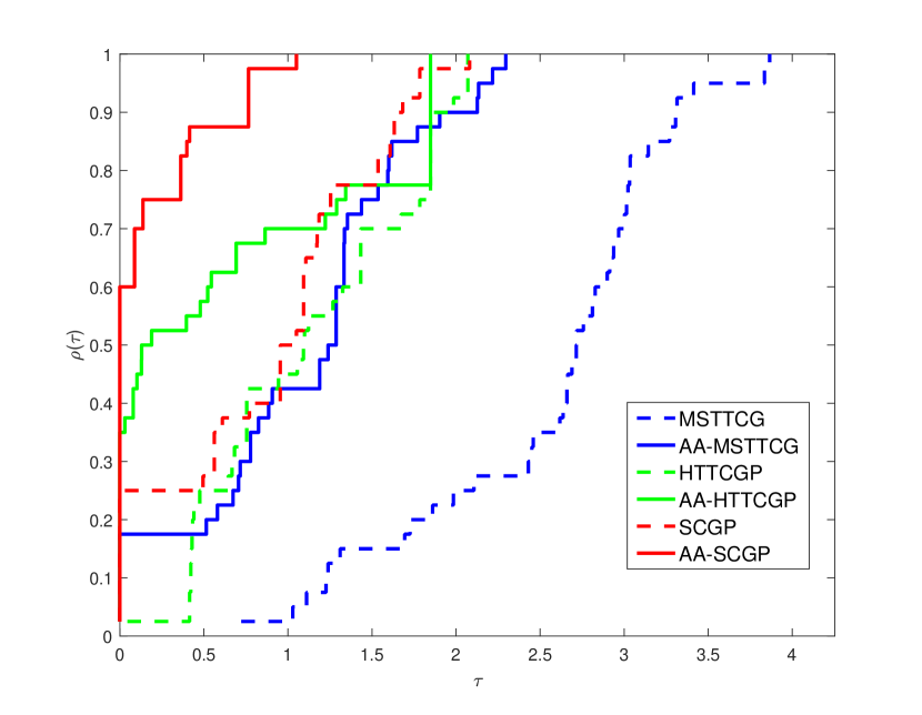
Moreover, we use the performance profiles DM02 to visually compare the performance of these methods, as illustrated in Figures 1(a) and 1(b), which intuitively describe $\overline{\rm Iter}$ and $\overline{\rm NF}$ , respectively. Recall that in the performance profile, efficiency and robustness can be evaluated at the left and right extremes of the graphic, respectively. In a word, the higher the curve, the better the method. It is very clear from Figure 1 that the acceleration process is efficient in its purpose of accelerating DFPM. Table 1 shows that the AA variants of three DFPM are all superior (in terms of $\overline{\rm Iter}$ , $\overline{\rm NF}$ and $\overline{\|F^{\ast}\|}$ ) to their originals for these chosen set of test problems, which also confirms the encouraging capability of AA for DFPM. In contrast, $\overline{\rm Tcpu}$ deteriorates in certain tests as a result of AA having to solve an extra optimization problem in each iteration. These results motivated us to further apply AA-DFPM to real-world problems.

5.2 Regularized decentralized logistic regression

We consider a real-world application, regularized decentralized logistic regression:

\min_{x\in\mathbb{R}^{n}}f(x):=\frac{1}{M}\sum_{i=1}^{M}\ln(1+\exp(-b_{i}a_{i}^{\top}x))+\frac{\tau}{2}\|x\|^{2},

(33)

where $\tau>0$ is a regularization parameter, $\frac{1}{M}\sum\limits_{i=1}^{M}\ln(1+\exp(-b_{i}a_{i}^{\top}x))$ represents the logistic loss function, and the data pairs $(a_{i},b_{i})\in\mathbb{R}^{n}\times\{-1,1\}(i=1,\ldots,M)$ are taken from a given data set or distribution. It is easy to know that the objective function $f$ is strongly convex Luo21 . Hence $x^{*}\in\mathbb{R}^{n}$ is a unique optimal solution to (33) if and only if it is a root of the following monotone nonlinear equations JYTH22 ,

F(x):=\nabla f(x)=\frac{1}{M}\sum_{i=1}^{M}\frac{-b_{i}\exp(-b_{i}a_{i}^{\top}x)a_{i}}{1+\exp(-b_{i}a_{i}^{\top}x)}+\tau x=0.

(34)

Thus we can apply AA-DFPM to solve the above problem. Considering that problem (34) is unconstrained, we can dispense with the nonnegative constraints in the least squares problem in Algorithm 3 (line 3 of Step 5), let $a^{k}_{k}=1-\sum\limits_{j=k-{m_{k}}}^{k-1}a^{k}_{j}$ , so the least squares problem can be reformulated as

\min\limits_{(a^{k}_{k-{m_{k}}},\dots,a^{k}_{k-1})^{\top}}\left\|r_{k}+\sum\limits_{j=k-{m_{k}}}^{k-1}a^{k}_{j}(r_{j}-r_{k})\right\|^{2}.

(35)

Our implementation solves above problem using QR decomposition. The QR decomposition of problem (35) at iteration $k$ can be efficiently obtained from that of at iteration $k-1$ in $O(m_{k}n)$ GVL96 .

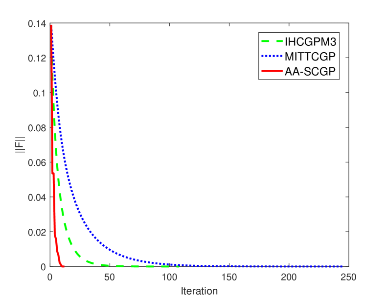
We exclusively focus on AA-SCGP, the top-performing method in our initial experiments, and compare it with two DFPM incorporating inertial acceleration: MITTCGP MJJYH23 and IHCGPM3 JYTH22 . The involved parameters for both MITTCGP and IHCGPM3 are set to their defaults, while the parameters used in AA-SCGP are taken from the experiment in last subsection. The regularization parameter is fixed at $\tau=0.01$ and the test instances are sourced from the LIBSVM data sets CL11 . Statistics of the test instances ¹¹1Datasets available at https://www.csie.ntu.edu.tw/ $\sim$ cjlin/libsvmtools/datasets/. used are listed in Table 2. The termination criterion of all three algorithms is the same as the first experiment.

Table 2: Numerical results on the LIBSVM test instances

Data sets	Data points	Variables	IHCGPM3	MITTCGP	AA-SCGP
Data sets	$M$	$n$	$\overline{\rm Iter}$ / $\overline{\rm NF}$ / $\overline{\rm Tcpu}$ / $\overline{\\|F^{\ast}\\|}$	$\overline{\rm Iter}$ / $\overline{\rm NF}$ / $\overline{\rm Tcpu}$ / $\overline{\\|F^{\ast}\\|}$	$\overline{\rm Iter}$ ( $\overline{\rm NAA}$ )/ $\overline{\rm NF}$ / $\overline{\rm Tcpu}$ / $\overline{\\|F^{\ast}\\|}$
fourclass_scale	862	2	107.6/323.8/0.017/9.60e-07	246.6/740.4/0.038/9.82e-07	11.4(10.0)/23.8/0.011/2.18e-07
liver-disorders	145	5	492.2/1520.6/0.023/9.93e-07	1362.6/4136.8/0.065/9.98e-07	760.0(462.4)/2086.4/0.088/7.70e-07
phishing	11055	68	561.8/1685.6/14.016/9.93e-07	1394.0/4182.6/34.768/9.97e-07	565.0(243.4)/1131.0/13.651/5.14e-07
w4a	7366	300	584.6/1754.8/2.815/9.92e-07	1461.4/4384.4/7.050/9.97e-07	628.0(309.0)/1257.2/3.104/9.11e-07
w5a	9888	300	584.0/1752.6/3.714/9.95e-07	1459.8/4380.0/9.226/9.98e-07	520.0(87.0)/1041.0/3.039/9.53e-07
w6a	17188	300	584.4/1753.0/8.294/9.95e-07	1460.2/4381.6/20.713/9.96e-07	757.2(575.8)/1515.4/12.007/7.83e-07

Figure 2 displays the results of four test instances solved by three methods with a fixed initial point $(0,\dots,0)^{\top}$ . One can observe that our method outperforms the others. Specifically, for different categories of data sets, AA-SCGP performs better in the case that has fewer data points $M$ and variables $n$ . The reason for this could be that data set “fourclass_scale” has been scaled to [-1,1]. For similar data sets “w5a” and “w6a”, AA-SCGP exhibits faster convergence for a bigger $M$ . Similarly, we use the MATLAB script “2*(rand(n,1)-0.5)” to generate the random initial point and run the same test 5 times for each test instance. Table 2 presents the average computational results, with the additional term $\overline{\rm NAA}$ denoting average number of AA. The results indicate that the quality of solutions obtained by AA-SCGP consistently outperforms those generated by IHCGPM3 and MITTCGP. For most test instances, AA-SCGP outperforms the other two inertial algorithms in terms of $\overline{\rm NF}$ and $\overline{\rm Tcpu}$ . This benefits from the fact that AA-SCGP accelerates frequently during its iteration, in which the proportion of AA is 55.6%. These facts further illustrate that DFPM integrated with Anderson acceleration is valid and promising.

6 Conclusions

In this paper, we developed a novel algorithm of using Anderson acceleration (AA) for derivative-free projection method (DFPM) in solving convex-constrained monotone nonlinear equations. First, we reviewed the convergence of a general framework for DFPM, and then explored how AA can still be exploited with DFPM though it may not a fixed-point iteration. As a result, an acceleration algorithm (AA-DFPM) with slight modifications is proposed, and the global convergence of AA-DFPM is obtained with no additional assumptions. The convergence rate is further established based on some suitable conditions. The results on both preliminary numerical experiments and applications demonstrate the superior performance. As a future research, we plan to investigate a novel DFPM for general nonlinear equations without the monotonicity. We also intend to explore a simplified AA whose coefficient is easy to calculate, even for large window size.

Acknowledgements.

This work was supported by the National Key Research and Development Program (2020YFA0713504) and the National Natural Science Foundation of China (61977065).

References

(1) Meintjes, K., Morgan, A.P.: A methodology for solving chemical equilibrium systems. Appl. Math. Comput. 2(4), 333-361 (1987)
(2) Qu, B., Xiu, N.H.: A note on the CQ algorithm for the split feasibility problem. Inverse Probl. 21(5), 1655-1665 (2005)
(3) Chorowski, J., Zurada, J.M.: Learning understandable neural networks with nonnegative weight constraints. IEEE Trans. Neural Netw. Learn. Syst. 26(1), 62-69 (2014)
(4) Xiao, Y.H., Wang, Q.Y., Hu, Q.J.: Non-smooth equations based method for $\ell_{1}$ -norm problems with applications to compressed sensing. Nonlinear. Anal. 74(11), 3570-3577 (2011)
(5) Jian, J.B., Yin, J.H., Tang, C.M., Han, D.L.; A family of inertial derivative-free projection methods for constrained nonlinear pseudo-monotone equations with applications. Comp. Appl. Math. 41, 309 (2022)
(6) Sun, D.F., Womersley, R.S., Qi, H.D.: A feasible semismooth asymptotically Newton method for mixed complementarity problems. Math. Program. 94(1), 167-187 (2002)
(7) Qi, L.Q., Tong, X.J., Li, D.H.: Active-set projected trust-region algorithm for boxconstrained nonsmooth equations. J. Optim. Theory Appl. 120(3), 601-625 (2004)
(8) Yin, J.H., Jian, J.B., Ma, G.D.: A modified inexact Levenberg-Marquardt method with the descent property for solving nonlinear equations. Comput. Optim. Appl. 87, 289-322 (2023)
(9) Solodov, M.V., Svaiter, B.F.: A globally convergent inexact Newton method for systems of monotone equations. In: Fukushima, M., Qi. L. (eds.): Reformulation: Nonsmooth, Piecewise Smooth, Semisooth and Smoothing Methods, pp. 355-369. Kluwer, Dordrecht (1998)
(10) Liu, J.K., Feng, Y.M.: A derivative-free iterative method for nonlinear monotone equations with convex constraints. Numer. Algorithms 82, 245-262 (2019)
(11) Liu, J.K., Lu, Z.L., Xu, J.L., Wu, S., Tu, Z.W., An efficient projection-based algorithm without Lipschitz continuity for large-scale nonlinear pseudo-monotone equations. J. Comput. Appl. Math. 403, 113822 (2022)
(12) Ibrahim, A.H., Kumam, P., Rapajić, S., Papp, Z., Abubakar, A.B.: Approximation methods with inertial term for large-scale nonlinear monotone equations. Appl. Numer. Math. 181, 417-435 (2022)
(13) Wu, X.Y., Shao, H., Liu, P.J., Zhuo, Y.: An inertial spectral CG projection method based on the memoryless BFGS update. J. Optim. Theory Appl. 198, 1130-1155 (2023)
(14) Yin, J.H., Jian, J.B., Jiang, X.Z., Liu, M.X., Wang, L.Z.: A hybrid three-term conjugate gradient projection method for constrained nonlinear monotone equations with applications. Numer. Algorithms 88(1), 389-418(2021)
(15) Waziri, M.Y., Ahmed, K.: Two descent Dai-Yuan conjugate gradient methods for systems of monotone nonlinear equations. J. Sci. Comput. 90, 1-53 (2022)
(16) Ma, G.D., Jin, J.C., Jian, J.B., Yin, J.H., Han, D.L.: A modified inertial three-term conjugate gradient projection method for constrained nonlinear equations with applications in compressed sensing. Numer. Algorithms 92, 1621-1653 (2023)
(17) Zhang, L., Zhou, W.J.: Spectral gradient projection method for solving nonlinear monotone equations. J. Comput. Appl. Math. 196, 478-484 (2006)
(18) Ou, Y.G.; Li, J.Y.: A new derivative-free SCG-type projection method for nonlinear monotone equations with convex constraints. J. Appl. Math. Comput. 56, 195-216 (2018)
(19) Amini, K., Kamandi, A.: A new line search strategy for finding separating hyperplane in projection-based methods. Numer. Algorithms 70, 559-570 (2015)
(20) Li, Q.N., Li, D.H.: A class of derivative-free methods for large-scale nonlinear monotone equations. IMA J. Numer. Anal. 31(4), 1625-1635 (2011)
(21) Ou, Y.G., Li, L.: A unified convergence analysis of the derivative-free projection-based method for constrained nonlinear monotone equations. Numer. Algorithms 93(4), 1639-1660 (2023)
(22) Goncalves, M.L.N., Menezes, T.C.: A framework for convex-constrained monotone nonlinear equations and its special cases. Comp. Appl. Math. 42, 306 (2023)
(23) Anderson, D.G.; Iterative procedures for nonlinear integral equations. J. Assoc. Comput. Mach. 12 547-560 (1965)
(24) Alvarez, F.: On the minimizing property of a second order dissipative system in Hilbert spaces. SIAM J. Control Optim. 38(4), 1102-1119 (2000)
(25) Nesterov, Y.: A method of solving a convex programming problem with convergence rate $O(1/k^{2})$ . Soviet Math. Dokl. 27, 372-376 (1983)
(26) Walker, H.F., Ni, P.: Anderson acceleration for fixed-point iterations. SIAM J. Numer. Anal. 49(4), 1715-1735 (2011)
(27) Saad, Y., Schultz, M.H.: Gmres: A generalized minimal residual algorithm for solving nonsymmetric linear systems. SIAM J. Sci. Stat. Comput. 7(3), 856-869 (1986)
(28) Potra, F.A., Engler, H.: A characterization of the behavior of the Anderson acceleration on linear problems. Linear Algebra Appl. 438(3), 1002-1011 (2013)
(29) Wang, D.W., He, Y.H., Sterck, H.D.: On the asymptotic linear convergence speed of Anderson acceleration applied to ADMM. J. Sci. Comput. 88(2), 38 (2021)
(30) Fang, H.R., Saad, Y.: Two classes of multisecant methods for nonlinear acceleration. Numer. Linear Algebra Appl. 16(3), 197-221 (2009)
(31) Wang, S.Y., Chen, W.Y., Huang, L.W., Zhang, F., Zhao, Z.T., Qu, H.: Regularization-adapted Anderson acceleration for multi-agent reinforcement learning, Knowl.-Based Syst. 275, 110709 (2023)
(32) Pollock, S., Rebholz, L.G., Xiao, M.Y.: Anderson-accelerated convergence of Picard iterations for incompressible Navier-Stokes equations. SIAM J. Numer. Anal. 57, 615-637 (2019)
(33) Yang, Y.N.: Anderson acceleration for seismic inversion. Geophysics 86(1), R99-R108 (2021)
(34) Toth, A., Kelley, C.: Convergence analysis for Anderson acceleration. SIAM J. Numer. Anal. 53, 805-819 (2015)
(35) Mai, V., Johansson, M.: Anderson acceleration of proximal gradient methods. In Int. Conf. Mach. Learn., PMLR, 6620-6629 (2020)
(36) Bian, W., Chen, X.J.: Anderson acceleration for nonsmooth fixed point problems. SIAM J. Numer. Anal. 60(5), 2565-2591 (2022)
(37) Rebholz, L.G., Xiao, M.Y.: The effect of Anderson acceleration on superlinear and sublinear convergence. J. Sci. Comput. 96(2), 34 (2023)
(38) Garner, C., Lerman, G., Zhang, T.: Improved convergence rates of Anderson acceleration for a large class of fixed-point iterations. arXiv preprint arXiv: 2311.02490 (2023).
(39) Cai, X.J., Gu, G.Y., He, B.S.: On the $O(1/t)$ convergence rate of the projection and contraction methods for variational inequalities with Lipschitz continuous monotone operators. Comput. Optim. Appl. 57(2), 339-363 (2014)
(40) Polyak, B.T.: Introduction to Optimization, Optimization Software, Inc. Publications Division, New York (1987).
(41) Scieur, D., d’Aspremont, A., Bach, F.: Regularized nonlinear acceleration. In Adv. Neural Inf. Process. Syst. 712-720 (2016)
(42) Ouyang, W.Q., Tao, J., Milzarek, A., Deng, B.L.: Nonmonotone globalization for Anderson Acceleration via adaptive regularization. J. Sci. Comput. 96, 5 (2023)
(43) Henderson, N.C., Varadhan, R.: Damped Anderson acceleration with restarts and monotonicity control for accelerating EM and EM-like algorithms. J. Comput. Graph. Stat. 28, 834-846 (2019)
(44) Ouyang, W.Q., Peng, Y., Yao, Y.X., Zhang, J.Y., Deng, B.L.: Anderson acceleration for nonconvex ADMM based on Douglas-Rachford splitting. Comput. Graph. Forum 39, 221-239 (2020)
(45) Zhang, J.Y., O’Donoghue, B., Boyd, S.: Globally convergent type-I Anderson acceleration for nonsmooth fixed-point iterations. SIAM J. Optim. 30(4), 3170-3197 (2020)
(46) Anderson, D.G.M.: Comments on “Anderson Acceleration, Mixing and Extrapolation”. Numer. Algorithms 80, 135-234 (2019)
(47) Chen, C.H., Ma, S.Q., Yang, J.F.: A general inertial proximal point algorithm for mixed variational inequality problem. SIAM J. Optim. 25, 2120-2142 (2014)
(48) Amini, K., Faramarzi, P.: Global convergence of a modified spectral three-term CG algorithm for nonconvex unconstrained optimization problems. J. Comput. Appl. Math. 417, 114630 (2023)
(49) Dolan, E.D., Moré, J.J.: Benchmarking optimization software with performance profiles. Math. Program. 91(2), 201-213 (2002)
(50) Luo, H.: Accelerated primal-dual methods for linearly constrained convex optimization problems. arXiv preprint arXiv: 2109.12604 (2021).
(51) Golub, G.H., Van Loan, C.: Matrix Computations, 3rd ed., The Johns Hopkins University Press, Baltimore, MD, (1996)
(52) Chang, C.C., Lin, C.J.: LIBSVM: a library for support vector machines. ACM Trans. Intell. Syst. Technol. 2(3), 1-27 (2011)

$\displaystyle\\|x_{k+1}-x^{*}\\|^{2}=$	$\displaystyle\\|P_{\mathcal{C}}[x_{k}-\zeta u_{k}F(z_{k})]-P_{\mathcal{C}}[x^{*}]\\|^{2}$
$\displaystyle\leq$	$\displaystyle\\|x_{k}-\zeta u_{k}F(z_{k})-x^{*}\\|^{2}$
$\displaystyle=$	$\displaystyle\\|x_{k}-x^{}\\|^{2}-2\zeta u_{k}F(z_{k})^{\top}(x_{k}-x^{})+\zeta^{2}u_{k}^{2}\\|F(z_{k})\\|^{2}$
$\displaystyle\overset{\eqref{vz}}{\leq}$	$\displaystyle\\|x_{k}-x^{*}\\|^{2}-2\zeta u_{k}F(z_{k})^{\top}(x_{k}-z_{k})+\zeta^{2}u_{k}^{2}\\|F(z_{k})\\|^{2}$
$\displaystyle=$	$\displaystyle\\|x_{k}-x^{*}\\|^{2}-\zeta(2-\zeta)\frac{(F(z_{k})^{\top}(x_{k}-z_{k}))^{2}}{\\|F(z_{k})\\|^{2}}$
$\displaystyle\overset{\eqref{vz}}{\leq}$	$\displaystyle\\|x_{k}-x^{*}\\|^{2}-\zeta(2-\zeta)\frac{\sigma^{2}t_{1}^{2}\alpha_{k}^{4}\\|d_{k}\\|^{4}}{\\|F(z_{k})\\|^{2}}.$	(12)

	$\displaystyle\\|x_{k}^{a}-x^{*}\\|$	$\displaystyle=\left\\|\sum\limits_{j=k-{m_{k}}}^{k}a^{k}_{j}x_{j}-x^{}\right\\|=\left\\|v_{k}-x^{}+\sum\limits_{j=k-{m_{k}}}^{k}a^{k}_{j}x_{j}-v_{k}\right\\|$
		$\displaystyle\leq\\|v_{k}-x^{*}\\|+\left\\|\sum\limits_{j=k-{m_{k}}}^{k}a^{k}_{j}x_{j}-v_{k}\right\\|.$		(13)

	$\displaystyle\\|x_{k}^{a}-x^{*}\\|^{2}$	$\displaystyle\overset{\eqref{xv}}{\leq}(\\|v_{k}-x^{}\\|+\\|x_{k}^{a}-v_{k}\\|)^{2}\leq(\\|v_{k}-x^{}\\|+c)^{2}$
		$\displaystyle=\\|v_{k}-x^{}\\|^{2}+2c\\|v_{k}-x^{}\\|+c^{2}\leq\\|v_{k}-x^{*}\\|^{2}+2cM+c^{2}.$		(16)

	$\displaystyle\\|x_{k+1}-x^{*}\\|^{2}=$	$\displaystyle\\|x_{k}^{a}-x^{*}+b_{k}(v_{k}^{a}-x_{k}^{a})\\|^{2}$
	$\displaystyle\leq$	$\displaystyle\\|x_{k}^{a}-x^{}\\|^{2}+(b_{k}\\|v_{k}^{a}-x_{k}^{a}\\|)^{2}+2b_{k}\\|v_{k}^{a}-x_{k}^{a}\\|\\|x_{k}^{a}-x^{}\\|$
	$\displaystyle\overset{\eqref{xaM}}{\leq}$	$\displaystyle\\|x_{k}^{a}-x^{*}\\|^{2}+(b_{k}\\|v_{k}^{a}-x_{k}^{a}\\|)^{2}+2(m+1)Mb_{k}\\|v_{k}^{a}-x_{k}^{a}\\|$
	$\displaystyle\overset{\eqref{xa2M}}{\leq}$	$\displaystyle\\|v_{k}-x^{*}\\|^{2}+2cM+c^{2}+(b_{k}\\|v_{k}^{a}-x_{k}^{a}\\|)^{2}+2(m+1)Mb_{k}\\|v_{k}^{a}-x_{k}^{a}\\|$
	$\displaystyle\overset{\eqref{vx*}}{\leq}$	$\displaystyle\\|x_{k}-x^{*}\\|^{2}-\zeta(2-\zeta)\frac{\sigma^{2}t_{1}^{2}\alpha_{k}^{4}\\|d_{k}\\|^{4}}{\\|F(z_{k})\\|^{2}}+2cM+c^{2}$
		$\displaystyle+(b_{k}\\|v_{k}^{a}-x_{k}^{a}\\|)^{2}+2(m+1)Mb_{k}\\|v_{k}^{a}-x_{k}^{a}\\|.$

	$\displaystyle\zeta(2-\zeta)\frac{\sigma^{2}t_{1}^{2}}{N^{2}}\sum\limits_{k=0}^{\infty}(\alpha_{k}\\|d_{k}\\|)^{4}\leq$	$\displaystyle\sum\limits_{k=0}^{\infty}\left(\\|{x}_{k}-x^{}\\|^{2}-\\|x_{k+1}-x^{}\\|^{2}+2cM+c^{2}\right.$
		$\displaystyle\left.+(b_{k}\\|v_{k}^{a}-x_{k}^{a}\\|)^{2}+2(m+1)Mb_{k}\\|v_{k}^{a}-x_{k}^{a}\\|\right)$
	$\displaystyle=$	$\displaystyle\\|{x}_{0}-x^{}\\|^{2}-\lim\limits_{k\to\infty}\\|{x}_{k+1}-x^{}\\|^{2}+2cM+c^{2}$
		$\displaystyle+\sum\limits_{k=0}^{\infty}(b_{k}\\|v_{k}^{a}-x_{k}^{a}\\|)^{2}+2(m+1)M\sum\limits_{k=0}^{\infty}b_{k}\\|v_{k}^{a}-x_{k}^{a}\\|<\infty$