Anchor-based Multi-view Subspace Clustering with Hierarchical Feature Descent

The decision variables for the objective function are $\{\mathbf{W}^{(v)}_{i}\}_{i=1}^{\delta},\mathbf{A}$, $\mathbf{Z}$ and $\boldsymbol{\alpha}$. As a result, we introduce a four-step iterative optimization method to approximate the optimal target mentioned in Eq. (6). In this approach, we keep three variables fixed while optimizing the remaining ones. The specific procedure is derived from the following detailed steps.

Where $\boldsymbol{\Omega}$ denotes the hierarchical dimensional projection series $\mathbf{W}^{(v)}_{1}\mathbf{W}^{(v)}_{2}\cdots\mathbf{W}^{(v)}_{o-1}$. The multiplication term $\hat{\mathbf{A}}_{o}\mathbf{Z}$ refers to the anchor-based subspace reconstruction of $i$-th layer’s representation, and $\hat{\mathbf{A}}_{o}$ denotes the generalized anchors. Through deduction of matrix Frobenius norm and let $\mathbf{M}^{(v)}=\boldsymbol{\Omega}^{\top}\mathbf{X}^{(v)}\mathbf{Z}^{\top}\mathbf{A}^{\top}$, Eq. (3.2.1) can be reformulated as:

Denote the SVD of matrix $\mathbf{M}^{(v)}$ as $\mathbf{U}_{\mathbf{M}}\mathbf{D}_{\mathbf{M}}\mathbf{V}_{\mathbf{M}}^{\top}$ and the optimal solution of Eq. (9) is demonstrated as ${\mathbf{W}^{(v)}_{o}}^{\star}$. In this case, $\mathbf{D}_{\mathbf{M}}$ is a nonnegative diagonal matrix with each entry representing the singular value of $\mathbf{M}^{(v)}$, both $\mathbf{U}_{\mathbf{M}}$ and $\mathbf{V}_{\mathbf{M}}$ are unitary matrix with orthogonal entries. According to deduction in [23], a closed-form resolution can be found by calculating ${\mathbf{W}^{(v)}_{o}}^{\star}=\mathbf{U}_{\mathbf{M}}sign(\mathbf{D}_{\mathbf{M}})\mathbf{V}_{\mathbf{M}}^{\top}$, where $sign(\cdot)$ is a function imposed on matrix with each element, which returns $1$ if the element is larger than $0$. And it is obvious that in our case, $sign(\mathbf{D}_{\mathbf{M}})$ is an identity matrix. Accordingly, the optimal solution can be calculated as:

By following the updating expression in Eq. (10), our algorithm updates $\mathbf{W}^{(v)}_{i},~{}i=1,2,\cdots,\delta$ in succession.

Likewise, the deduction for the optimization of the anchor selection variable $\mathbf{A}$ is similar to Eq. (9), which can be equally written as:

where $\Phi=\sum_{v=1}^{p}\alpha_{v}^{2}{\mathbf{W}^{(v)}_{\delta}}^{\top}{\mathbf{W}^{(v)}_{\delta-1}}^{\top}\cdots{\mathbf{W}^{(v)}_{1}}^{\top}\mathbf{X}^{(v)}\mathbf{Z}^{\top}$ and $\Phi\in\mathbb{R}^{k\times m}$.

Corresponding to the updating rule in [23], it is straightforward to obtain the optimal solution for $\mathbf{A}$ as in Eq. (9). The multiplication of the left and right singular matrices of $\Phi$ costs $\mathcal{O}(km^{2})$.

According to the definition of Frobenius norm, we can easily derive Eq. (13) as follows:

where $\mathbf{P}=\mathbf{W}^{(v)}_{1}\mathbf{W}^{(v)}_{2}\cdots\mathbf{W}^{(v)}_{\delta}\mathbf{A}$. As the optimisation of the columns in $\mathbf{Z}$ is identical with each other, the optimisation task can be separated into $n$ sub-tasks by the identical form as:

for $j=1,2,\cdots,n$, where the parameter for quadratic term is $\mathbf{Q}=2\sum_{v=1}^{p}{\alpha_{v}^{2}}\mathbf{I}$ and the first order polynomial term ${\boldsymbol{q}^{\top}}=-2\sum_{v=1}^{p}{\alpha_{v}^{2}}{\mathbf{X}^{(v)}_{:,j}}^{\top}\mathbf{P}$. These are several QP(quadratic programming) problems with domain constraints. As each column of $\mathbf{Z}$ is an $m$ dimensional vector, and there are $n$ sub-problems identical to each other, the overall time cost of optimising $\mathbf{Z}$ is $\mathcal{O}(nm^{3})$.

Denote the Frobenius norm of the alignment term $(\mathbf{X}^{(v)}-\mathbf{W}^{(v)}_{1}\mathbf{W}^{(v)}_{2}\cdots\mathbf{W}^{(v)}_{\delta}\mathbf{A}\mathbf{Z})$ as $f^{(v)}$, and the vector $\mathbf{F}=[f^{(1)},f^{(2)},\cdots,f^{(m)}]^{\top}$ refers to the concatenation. By Cauchy-Schwarz inequality, the optimal value of $\boldsymbol{\alpha}$ can be directly acquired by

In our four-step iterative convex optimization process, each updating formula has a closed-form solution and for each iteration, the objective value of the optimization target monotonically decreases while keeping the rest of the decision variables fixed. At the same time, both $\{\mathbf{W}^{(v)}_{i}\}_{i=1}^{\delta}$ and $\mathbf{A}$ are orthogonal matrices, while both $\boldsymbol{\alpha}$ and $\mathbf{Z}$ satisfies $1$-sum non-negative constraints, which provides the lower bound of the optimization target. Consequently, the convex objective monotonically decreases with a lower bound, thus guaranteeing the overall convergence of the proposed method MVSC-HFD.

The optimization procedure demonstrated in Algorithm 1 has decomposed the model into four sub-problems with a closed-form solution. For simplicity and practicality, the hierarchical dimensional reduction processes are conducted identically for different views. Subsequently, their layers’ dimensions $\{l_{i}\}_{i=1}^{\delta}$ are the same. In specific, the optimization of $\mathbf{W}^{(v)}_{o}$ in Eq. (10) involves the calculation of $\mathbf{M}^{(v)}$ and its SVD complexity, which is $\mathcal{O}((\sum_{i=0}^{\delta-2}l_{i}l_{i+1})l_{\delta}+nd_{v}l_{\delta}+2md_{v}l_{\delta})$ and $\mathcal{O}(l_{o-1}k^{2})$, respectively. The multiplication applied to acquire $\mathbf{W}^{(v)}_{o}$ is $\mathcal{O}(l_{o-1}k^{2})$. In all, suppose the dimension $l_{\delta}$ of the last layer is the same as the cluster number $k$ and $\sum_{i=1}^{p}d_{v}=q$, it needs $\mathcal{O}((ql_{1}+p\sum_{i=0}^{\delta-2}l_{i}l_{i+1})k+nqk+2mqk)$ to update $\{\mathbf{W}^{(v)}_{i}\}_{i=1}^{\delta}$ for all views. The optimization of $\mathbf{A}$ requires $\mathcal{O}(k(d_{v}+m)n)$ time cost to gather the multiplicator and $\mathcal{O}(km^{2})$ to decompose it. In sum, the overall complexity of our algorithm is $\mathcal{O}(n)$, which is scalable for large-scale datasets.

For in-depth experimental analysis, we conduct a series of tests over 10 real-world datasets, varying in multiple domains. The datasets used in our experiments are WebKB ¹¹1http://lig-membres.imag.fr/grimal/data.html, BDGP ²²2https://www.fruitfly.org/, MSRCV1 [38], Caltech7-2view ³³3http://www.vision.caltech.edu/Image_Datasets/Caltech101/, NUS-WIDE-10 ⁴⁴4https://lms.comp.nus.edu.sg/wp-content/uploads/2019/research/nuswide/NUS-WIDE.html, Caltech101-7 ³, Caltech101-20 ³, NUS-WIDE ⁴, SUNRGBD ⁵⁵5https://rgbd.cs.princeton.edu/, YoutubeFace ⁶⁶6https://www.cs.tau.ac.il/ wolf/ytfaces/. These datasets vary in broad ranges of application background. In specific, WebKB is a dataset that includes web pages from computer science departments of various universities and they are categorized into 5 categories (Student, Faculty, Department, Course, Project). The SUNRGBD dataset contains 10335 real RGB-D images of room scenes. The MSRCV1 dataset from Microsoft Research in Cambridge contains 7 classes of images with coarse pixel-wise labeling. In Table 2, we summarize the detailed information of these benchmark datasets.

We use the initialization specified in Algorithm 1. In practice, we simply adopt the number of clusters $k$ as the value of the dimension of embedding space and the value of anchor count. For each view, the hierarchical feature descent rate is different according to their original dimensions. However, it is rather practicable as it performs well by directly slicing the dimension to equal sections: $l_{o}-l_{o-1}=l_{o+1}-l_{o},\forall o\in[1,\delta]$. The best depths among $[1,2,\cdots,5]$ of the datasets WebKB, BDGP, MSRCV1, Caltech7-2view, NUS-WIDE-10, Caltech101-7, Caltech101-20, NUS-WIDE ⁴, SUNRGBD, YoutubeFace are 5, 5, 5, 5, 4, 4, 5, 5, 2, respectively.

To be specific, the experiments are conducted in MATLAB environment on PC with Intel(R) Core(TM) i7-6800K 3.40GHz CPU and 128GB RAM.

We list the information of our compared algorithms as in detail as possible by first giving brief introduction to their distinct mechanism, and analyze the hyper-parameters of each method.

• 1.

  Multi-view k-means clustering on big data (RMKM) [5]. This method uses $\ell_{2,1}$ norm to minimize the non-negative matrix factorization form of the cluster indicator matrix in terms of reconstruction of the original data matrix. Its inherent property is similar to the $k$-means clustering method and the $1$-of-$K$ coding scheme provides one-step clustering results.

• 2.

  Large-scale multi-view subspace clustering in linear time (LM-
  VSC) [16]. Under the framework of subspace clustering, this paper intends for clustering of large-scale datasets by using initially selected anchor points to build reconstruction.

• 3.

  Parameter-free auto-weighted multiple graph learning: a fram-ework for multi-view clustering and semi-supervised classification (AMGL) [22]. A fusion of different graph representations where the weights of each graph of view are automatically learned and assumed to be the optimal combination.

• 4.

  Binary Multi-view Clustering (BMVC) [49]. In order to reduce computational complexity and spacial cost, this work proposes to integrate binary representation of all views and consensus binary clustering into a uniform framework by both minimizing these two parts of loss at the same time.

• 5.

  Flexible Multi-View Representation Learning for Subspace Clustering (FMR) [17]. After performing clustering on each different view, the best clustering result is flexibly encoded via adopting complementary information of provided views, thus avoiding the partial outcome in the reconstruction stage.

• 6.

  Multi-view Subspace Clustering (MVSC) [12]. MVSC proposes to learn subspace representation of different views simultaneously while regularising the separate affinity matrices to a common one to improve clustering consistency among different views.

• 7.

  Multi-view clustering: A scalable and parameter-free bipartite graph fusion method (SFMC) [18]. Based on Ky Fan’s Theorem [10], SFMC explores the relationship between Laplacian matrix and graph connectivity, thus proposing a scalable and parameter-free method to interactively fuse the view-specific graphs into a consensus graph with adaptable anchor strategy.

• 8.

  Fast parameter-free multi-view subspace clustering with consensus anchor guidance (FPMVS-CAG) [33]. FPMVS-CAG integrates anchor guidance and bipartite graph construction within an optimization framework and learns collaboratively, promoting clustering quality. The algorithm offers linear time complexity, is hyper-parameter-free, and automatically learns an optimal anchor subspace graph.

• 9.

  Efficient Multi-view K-means Clustering with Multiple Anchor Graphs (EMKMC) [46]. EMKMC integrates anchor graph-based and $k$-means-based approaches, constructing anchor graphs for each view and utilizing an improved $k$-means strategy for integration. This enables high efficiency, particularly for large-scale high-dimensional multi-view data, while maintaining or surpassing clustering effectiveness compared to other methods.

As shown in Table.3, most of algorithm have more than one hyper-parameters. It is encouraged to use learnable parameters which can adaptively collaborate with the optimization of other decision variables to boost the performance whereas spare the acquisition of prior knowledge. In our method, the learnable vector of parameters $\boldsymbol{\alpha}=[\alpha_{1},\alpha_{2},\cdots,\alpha_{p}]^{\top}$ represents the weights adherent to different views, and they are optimized in each iteration. However, for the compared algorithm EMKMC, each view has a hyper-parameter, so the number of parameters is equal to the number of views, which we denote by $p$. As a result, the searching space for best parameter is $\epsilon^{p}$ where $\epsilon$ denotes the size of the candidate set of the hyper-parameter. These unlearnable parameters dramatically increases computation time of EMKMC.

The running time of compared algorithms on benchmark datasets are shown in Figure 4. Due to the excessive time consumed by some of the algorithms, we use the logarithms of the time as the vertical axis of the coordinate.

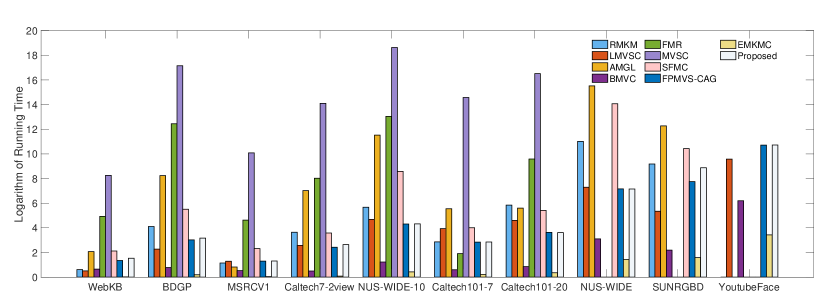
It is worth noticing that for large-scale datasets, namely NUS-WIDE, SUNRGBD and YoutubeFace, some algorithms(FMR, MVSC, SFMC, RMKM) encounter the ’Out-of-Memory’ problem. As a result, the time bars of these methods are omitted in the comparison graph. We observe that the time cost of EMKMC is comparable to ours, but the total runtime cost is still high owing to the aforementioned search space for the best hyper-parameters.

As described in the previous sections, our proposed algorithm possesses a theoretical guarantee, ensuring its convergence to a local minimum. Furthermore, to provide empirical evidence of its convergence, we conduct experiments on benchmark datasets. Figure 5 illustrates the evolution of the objective value throughout the experimental process. Notably, the experimental results reveal a consistent and monotonically decreasing trend in the objective values of our algorithm at each iteration. Furthermore, we observe that the algorithm achieves rapid convergence, typically within fewer than 10 iterations. These findings undeniably validate the convergence property of our proposed algorithm.

To demonstrate the impact of varying selections for the number of hierarchical dimension projection matrix, we present the performance variation across distinct layers of $\mathbf{W}^{(v)}_{i}$ with respect to each dataset, as depicted in Figure 6.

References

- Akaho [2006] Akaho, S., 2006. A kernel method for canonical correlation analysis. CoRR abs/cs/0609071.
- Andrew et al. [2013] Andrew, G., Arora, R., Bilmes, J.A., Livescu, K., 2013. Deep canonical correlation analysis, in: Proceedings of the 30th International Conference on Machine Learning, ICML 2013, Atlanta, GA, USA, 16-21 June 2013, JMLR.org. pp. 1247–1255.
- Bellman [1954] Bellman, R., 1954. Some applications of the theory of dynamic programming - A review. Oper. Res. , 275–288.
- Cai et al. [2023] Cai, X., Huang, D., Zhang, G.Y., Wang, C.D., 2023. Seeking commonness and inconsistencies: A jointly smoothed approach to multi-view subspace clustering. Information Fusion 91, 364–375.
- Cai et al. [2013] Cai, X., Nie, F., Huang, H., 2013. Multi-view k-means clustering on big data, in: Twenty-Third International Joint conference on artificial intelligence.
- Cao et al. [2015] Cao, X., Zhang, C., Fu, H., Liu, S., Zhang, H., 2015. Diversity-induced multi-view subspace clustering, in: IEEE Conference on Computer Vision and Pattern Recognition, CVPR 2015, Boston, MA, USA, June 7-12, 2015.
- Chen and Cai [2011] Chen, X., Cai, D., 2011. Large scale spectral clustering with landmark-based representation, in: Twenty-fifth AAAI conference on artificial intelligence.
- Chen et al. [2022] Chen, Z., Lin, P., Chen, Z., Ye, D., Wang, S., 2022. Diversity embedding deep matrix factorization for multi-view clustering. Information Sciences 610, 114–125.
- Elhamifar and Vidal [2013] Elhamifar, E., Vidal, R., 2013. Sparse subspace clustering: Algorithm, theory, and applications. IEEE Trans. Pattern Anal. Mach. Intell. .
- Fan [1949] Fan, K., 1949. On a theorem of weyl concerning eigenvalues of linear transformations i. Proceedings of the National Academy of Sciences 35, 652–655.
- Gao et al. [2015a] Gao, H., Nie, F., Li, X., Huang, H., 2015a. Multi-view subspace clustering, in: 2015 IEEE International Conference on Computer Vision, ICCV 2015, Santiago, Chile, December 7-13, 2015.
- Gao et al. [2015b] Gao, H., Nie, F., Li, X., Huang, H., 2015b. Multi-view subspace clustering, in: Proceedings of the IEEE international conference on computer vision, pp. 4238–4246.
- Guo [2013] Guo, Y., 2013. Convex subspace representation learning from multi-view data, in: Proceedings of the Twenty-Seventh AAAI Conference on Artificial Intelligence, July 14-18, 2013, Bellevue, Washington, USA, AAAI Press.
- Hotelling [1992] Hotelling, H., 1992. Relations between two sets of variates, in: Breakthroughs in statistics. Springer, pp. 162–190.
- Huang et al. [2021] Huang, S., Tsang, I.W., Xu, Z., Lv, J., Liu, Q., 2021. CDD: multi-view subspace clustering via cross-view diversity detection, in: MM ’21: ACM Multimedia Conference, Virtual Event, China, October 20 - 24, 2021, ACM. pp. 2308–2316.
- Kang et al. [2020] Kang, Z., Zhou, W., Zhao, Z., Shao, J., Han, M., Xu, Z., 2020. Large-scale multi-view subspace clustering in linear time, in: Proceedings of the AAAI Conference on Artificial Intelligence, pp. 4412–4419.
- Li et al. [2019] Li, R., Zhang, C., Hu, Q., Zhu, P., Wang, Z., 2019. Flexible multi-view representation learning for subspace clustering., in: IJCAI, pp. 2916–2922.
- Li et al. [2020] Li, X., Zhang, H., Wang, R., Nie, F., 2020. Multi-view clustering: A scalable and parameter-free bipartite graph fusion method. IEEE Transactions on Pattern Analysis and Machine Intelligence .
- Li et al. [2015] Li, Y., Nie, F., Huang, H., Huang, J., 2015. Large-scale multi-view spectral clustering via bipartite graph, in: Proceedings of the Twenty-Ninth AAAI Conference on Artificial Intelligence, January 25-30, 2015, AAAI Press. pp. 2750–2756.
- Liang et al. [2022] Liang, W., Liu, X., Zhou, S., Liu, J., Wang, S., Zhu, E., 2022. Robust graph-based multi-view clustering, in: Proceedings of the AAAI Conference on Artificial Intelligence, pp. 7462–7469.
- Liu et al. [2013] Liu, G., Lin, Z., Yan, S., Sun, J., Yu, Y., Ma, Y., 2013. Robust recovery of subspace structures by low-rank representation. IEEE Trans. Pattern Anal. Mach. Intell. .
- Nie et al. [2016] Nie, F., Li, J., Li, X., et al., 2016. Parameter-free auto-weighted multiple graph learning: a framework for multiview clustering and semi-supervised classification., in: IJCAI, pp. 1881–1887.
- Ou et al. [2020] Ou, Q., Wang, S., Zhou, S., Li, M., Guo, X., Zhu, E., 2020. Anchor-based multiview subspace clustering with diversity regularization. IEEE MultiMedia 27, 91–101.
- Qaqish et al. [2017] Qaqish, B.F., O’Brien, J.J., Hibbard, J.C., Clowers, K.J., 2017. Accelerating high-dimensional clustering with lossless data reduction. Bioinform. 33, 2867–2872.
- Shakhnarovich [2005] Shakhnarovich, G., 2005. Learning task-specific similarity. Ph.D. thesis. Massachusetts Institute of Technology, Cambridge, MA, USA.
- Shu et al. [2022] Shu, X., Zhang, X., Gao, Q., Yang, M., Wang, R., Gao, X., 2022. Self-weighted anchor graph learning for multi-view clustering. IEEE Transactions on Multimedia .
- Tang et al. [2023a] Tang, C., Li, Z., Wang, J., Liu, X., Zhang, W., Zhu, E., 2023a. Unified one-step multi-view spectral clustering. IEEE Trans. Knowl. Data Eng. 35, 6449–6460.
- Tang et al. [2023b] Tang, C., Sun, K., Tang, C., Zheng, X., Liu, X., Huang, J., Zhang, W., 2023b. Multi-view subspace clustering via adaptive graph learning and late fusion alignment. Neural Networks 165, 333–343.
- Tang et al. [2022] Tang, C., Zheng, X., Liu, X., Zhang, W., Zhang, J., Xiong, J., Wang, L., 2022. Cross-view locality preserved diversity and consensus learning for multi-view unsupervised feature selection. IEEE Trans. Knowl. Data Eng. 34, 4705–4716.
- Tang et al. [2023c] Tang, C., Zheng, X., Zhang, W., Liu, X., Zhu, X., Zhu, E., 2023c. Unsupervised feature selection via multiple graph fusion and feature weight learning. Sci. China Inf. Sci. 66.
- Wang et al. [2020] Wang, B., Xiao, Y., Li, Z., Wang, X., Chen, X., Fang, D., 2020. Robust self-weighted multi-view projection clustering, in: Proceedings of the AAAI Conference on Artificial Intelligence, pp. 6110–6117.
- Wang et al. [2016] Wang, M., Fu, W., Hao, S., Tao, D., Wu, X., 2016. Scalable semi-supervised learning by efficient anchor graph regularization. IEEE Transactions on Knowledge and Data Engineering 28, 1864–1877.
- Wang et al. [2021] Wang, S., Liu, X., Zhu, X., Zhang, P., Zhang, Y., Gao, F., Zhu, E., 2021. Fast parameter-free multi-view subspace clustering with consensus anchor guidance. IEEE Transactions on Image Processing 31, 556–568.
- Wang et al. [2017] Wang, X., Guo, X., Lei, Z., Zhang, C., Li, S.Z., 2017. Exclusivity-consistency regularized multi-view subspace clustering, in: 2017 IEEE Conference on Computer Vision and Pattern Recognition, CVPR 2017, IEEE Computer Society. pp. 1–9.
- Wang et al. [2015] Wang, Y., Lin, X., Wu, L., Zhang, W., Zhang, Q., Huang, X., 2015. Robust subspace clustering for multi-view data by exploiting correlation consensus. IEEE Trans. Image Process. 24, 3939–3949.
- Wang et al. [2018] Wang, Y., Wu, L., Lin, X., Gao, J., 2018. Multiview spectral clustering via structured low-rank matrix factorization. IEEE Trans. Neural Networks Learn. Syst. 29, 4833–4843.
- Wei et al. [2023] Wei, W., Yue, Q., Feng, K., Cui, J., Liang, J., 2023. Unsupervised dimensionality reduction based on fusing multiple clustering results. IEEE Trans. Knowl. Data Eng. 35, 3211–3223.
- Winn and Jojic [2005] Winn, J., Jojic, N., 2005. Locus: Learning object classes with unsupervised segmentation, in: Tenth IEEE International Conference on Computer Vision (ICCV’05) Volume 1, IEEE. pp. 756–763.
- Xia et al. [2014] Xia, R., Pan, Y., Du, L., Yin, J., 2014. Robust multi-view spectral clustering via low-rank and sparse decomposition, in: Proceedings of the Twenty-Eighth AAAI Conference on Artificial Intelligence, July 27 -31, 2014, AAAI Press. pp. 2149–2155.
- Xu et al. [2013] Xu, C., Tao, D., Xu, C., 2013. A survey on multi-view learning. CoRR abs/1304.5634.
- Yan et al. [2023a] Yan, W., Gu, M., Ren, J., Yue, G., Liu, Z., Xu, J., Lin, W., 2023a. Collaborative structure and feature learning for multi-view clustering. Inf. Fusion 98, 101832.
- Yan et al. [2023b] Yan, W., Gu, M., Ren, J., Yue, G., Liu, Z., Xu, J., Lin, W., 2023b. Collaborative structure and feature learning for multi-view clustering. Information Fusion 98, 101832.
- Yan et al. [2022] Yan, W., Xu, J., Liu, J., Yue, G., Tang, C., 2022. Bipartite graph-based discriminative feature learning for multi-view clustering, in: MM ’22: The 30th ACM International Conference on Multimedia, 2022, ACM. pp. 3403–3411.
- Yan et al. [2023c] Yan, W., Zhang, Y., Lv, C., Tang, C., Yue, G., Liao, L., Lin, W., 2023c. Gcfagg: Global and cross-view feature aggregation for multi-view clustering, in: IEEE/CVF Conference on Computer Vision and Pattern Recognition, CVPR, 2023, IEEE. pp. 19863–19872.
- Yang et al. [2023] Yang, B., Wu, J., Zhang, X., Lin, Z., Nie, F., Chen, B., 2023. Robust anchor-based multi-view clustering via spectral embedded concept factorization. Neurocomputing .
- Yang et al. [2022a] Yang, B., Zhang, X., Li, Z., Nie, F., Wang, F., 2022a. Efficient multi-view k-means clustering with multiple anchor graphs. IEEE Transactions on Knowledge and Data Engineering .
- Yang et al. [2022b] Yang, B., Zhang, X., Nie, F., Wang, F., 2022b. Fast multiview clustering with spectral embedding. IEEE Transactions on Image Processing 31, 3884–3895.
- Yang et al. [2022c] Yang, H., Gao, Q., Xia, W., Yang, M., Gao, X., 2022c. Multiview spectral clustering with bipartite graph. IEEE Transactions on Image Processing 31, 3591–3605.
- Zhang et al. [2018] Zhang, Z., Liu, L., Shen, F., Shen, H.T., Shao, L., 2018. Binary multi-view clustering. IEEE transactions on pattern analysis and machine intelligence 41, 1774–1782.
- Zhao et al. [2023] Zhao, M., Yang, W., Nie, F., 2023. Auto-weighted orthogonal and nonnegative graph reconstruction for multi-view clustering. Information Sciences 632, 324–339.
- Zhou et al. [2021] Zhou, S., Ou, Q., Liu, X., Wang, S., Liu, L., Wang, S., Zhu, E., Yin, J., Xu, X., 2021. Multiple kernel clustering with compressed subspace alignment. IEEE Transactions on Neural Networks and Learning Systems .