Anchor-Assisted Intelligent Reflecting Surface Channel Estimation for Multiuser Communications
Abstract
Due to the passive nature of Intelligent Reflecting Surface (IRS), channel estimation is a fundamental challenge in IRS-aided wireless networks. Particularly, as the number of IRS reflecting elements and/or that of IRS-served users increase, the channel training overhead becomes excessively high. To tackle this challenge, we propose in this paper a new anchor-assisted two-phase channel estimation scheme, where two anchor nodes, namely A1 and A2, are deployed near the IRS for helping the base station (BS) to acquire the cascaded BS-IRS-user channels. Specifically, in the first phase, the partial channel state information (CSI), i.e., the element-wise channel gain square, of the BS-IRS link is obtained by estimating the BS-IRS-A1/A2 channels and the A1-IRS-A2 channel, separately. Then, in the second phase, by leveraging such partial knowledge of the BS-IRS channel that is common to all users, the individual cascaded BS-IRS-user channels are efficiently estimated. Simulation results demonstrate that the proposed anchor-assisted channel estimation scheme is able to achieve comparable mean-squared error (MSE) performance as compared to the conventional scheme, but with significantly reduced channel training time.
I Introduction
Recently, intelligent reflecting surface (IRS) has emerged as a promising technology to achieve high spectral and energy efficiency for future wireless networks [1], [2]. Specifically, IRS is a uniform planar array composed of a large number of low-cost, passive, and tunable reflecting elements. By adaptively varying the reflection coefficient of each element based on the user dynamic channels, IRS can achieve high beamforming and interference suppression gains cost-effectively [3]. As such, IRS has been studied recently in various wireless systems, including non-orthogonal multiple access (NOMA)[4], [5], simultaneous wireless information and power transfer (SWIPT) [6], [7], secrecy communications [8], [9], and so on.
To reap the performance gain of IRS, accurate channel state information (CSI) is required. However, the passive nature of IRS makes channel estimation fundamentally challenging in IRS-aided wireless networks. This is because without radio frequency (RF) chains, IRS can neither transmit nor receive pilot signals, thus the base station (BS)-IRS and IRS-user channels cannot be estimated separately. One alternative approach is to estimate the cascaded BS-IRS-user channel via element-wise on-off operation at each reflecting element [10], [11] or time-varying reflection patterns [12], [13]. However, by applying the above methods to estimate the cascaded channels of multiple users consecutively, the required pilot overhead is the product of the number of IRS reflecting elements and that of users, which is prohibitively large for the case of large IRS serving a high density of users nearby (e.g., in a hot spot scenario).
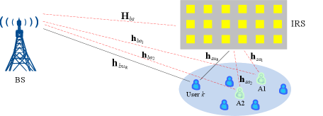
To tackle this problem, we propose in this paper a new anchor-assisted two-phase channel estimation scheme for IRS-aided multiuser communications, which can significantly reduce the channel training overhead by decoupling the estimation of cascaded channels and exploiting multiple antennas at the BS. As shown in Fig. 1, two anchor nodes, namely A1 and A2, are deployed near the IRS to assist its channel estimation. In the first phase, the cascaded BS-IRS-A1/A2 and A1-IRS-A2 channels are estimated separately, based on which the partial CSI of the BS-IRS link, in terms of the square of each IRS element’s channel with the BS (thus, with a +/- sign uncertainty), is obtained. In the second phase, with such partial CSI of the BS-IRS channel that is common to all users, the individual cascaded BS-IRS-user channels are efficiently estimated. Particularly, when the number of antennas at the BS () is no smaller than that () of the IRS reflecting elements, i.e. , we show that the proposed scheme can estimate all users’ cascaded channels in the second phase using only one pilot symbol. Besides, even for the case of , the minimum training overhead (in terms of number of pilot symbols) is shown to be , where is the number of IRS-served users and denotes the ceiling operation, which is significantly lower than for the conventional schemes [10, 11, 12, 13]. Moreover, in the case that the IRS-anchor channel is line-of-sight (LoS) by properly deploying the anchor, it is shown that the proposed scheme can be further simplified such that deploying only one anchor is sufficient.
II System Model
As shown in Fig. 1, we consider an IRS-assisted multiple-input-single-output (MISO) communication system, which consists of a BS, an IRS and users. The number of antennas at the BS and that of reflecting elements at the IRS are denoted by and , respectively. The channels from the BS to IRS and User are denoted by and , respectively, while that from the IRS to User is denoted by . We assume that two single-antenna anchor nodes111In practice, anchors can be idle user terminals and/or dedicated nodes such as adjacent IRS controllers. A1 and A2 are deployed near the IRS to assist in the channel estimation. The channels from the BS to A1 and A2 are denoted by and , respectively, those from the IRS to A1 and A2 are denoted by and , respectively, and that from A1 to A2 is denoted by . As a result, the cascaded BS-IRS-A1/A2/User channels are denoted by , and , respectively, while the cascaded A1-IRS-A2 channel is denoted by . Moreover, the phase-shift matrix of the IRS at time slot is denoted by , where is the reflection coefficient of the -th IRS element at time slot , . Since IRS is a passive reflecting device, we assume that the channel reciprocity holds for each link between IRS and any other node. The quasi-static flat-fading channel model is assumed for all the links involved.
III Anchor-assisted Channel Estimation
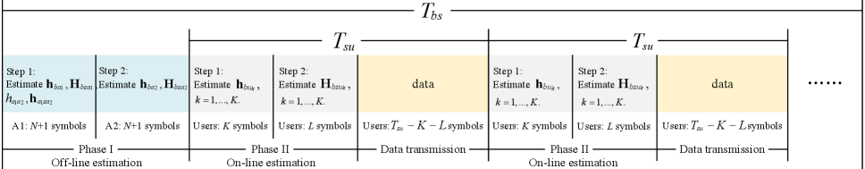
The proposed channel estimation and data transmission protocol is shown in Fig. 2, where and are the length of channel coherence block of and , , respectively, and for while for . In practice, is usually much larger than due to the fixed locations of the BS and IRS once deployed, while users can move randomly near the IRS. The channel estimation consists of one off-line phase (Phase I) and multiple on-line phases (each termed Phase II). In Phase I, the cascaded BS-IRS-A1, BS-IRS-A2, A1-IRS-A2 channels are estimated separately, which requires pilot symbols in total. In each Phase II, the BS estimates the cascaded BS-IRS-user channels with pilot symbols. For the estimation of in Phase II, the efficiency is largely improved, especially when increases up to . The detailed channel estimation scheme is elaborated as follows.
III-A Phase I: Off-line Estimation of
III-A1 Step 1
A1 transmits pilot symbol with power at time slot , then the received signals at the BS and A2 are respectively written as
| (1) |
| (2) |
Let , , , and . Then, (1) and (2) are rewritten as
| (3) |
| (4) |
There are in total unknowns in and the BS has observations at each time slot, thus A1 has to transmit pilot symbols at least for the BS to estimate . Similarly, it can be shown that at least pilot symbols are needed for A2 to estimate . By setting , and denoting , the overall received signals at the BS and A2 during the time slots are given by
| (5) |
| (6) |
where and , respectively. By properly constructing such that , and can be respectively estimated as
| (7) |
| (8) |
Practically, can be constructed based on the discrete Fourier transform (DFT) matrix [13], i.e.,
| (9) |
In this case, can be efficiently computed as by .
| (21) |
III-A2 Step 2
With , A2 transmits at least pilot symbols so that the BS can estimate as , similarly as in Step 1 and thus the details are omitted. With fed back from A2, BS obtains the estimated BS-IRS-A1, BS-IRS-A2 and A1-IRS-A2 channels, which are given by
| (10) | ||||
| (11) | ||||
| (12) |
Based on (10)-(12), the BS computes
| (13) |
where denotes the Hadamard product. By defining , is rewritten as
| (14) |
where . Letting , then each element in can be obtained as
| (15) |
i.e., we recover each but with a +/- sign uncertainty. However, we will show later that such partial CSI estimated is sufficient for resolving the cascaded channels ’s of all users uniquely.
III-B Phase II: On-line Estimation of and
III-B1 Step 1
users sequentially transmit one pilot symbol while the BS estimates , , respectively, where the details are omitted for brevity.
III-B2 Step 2
Users transmit pilot symbols while the BS estimates , , respectively. Denoting the pilot symbol transmitted from User at time slot by , the received signal at the BS is given by
| (16) |
Let , where and . Then, by removing the signal from the direct channel, can be re-expressed as
| (17) |
where
is the effective noise, including the channel estimation error in and . In conventional schemes [10, 11, 12, 13], pilot symbols are required to estimate each . However, in our proposed scheme, by leveraging the partial CSI of obtained in Phase I, the efficiency in estimating can be greatly improved. Specifically, we consider the following two cases.
Case 1: . In this case, users send pilot symbols consecutively for the BS to estimate , independently. Let , and . Then, is rewritten as
| (18) |
where and .
Since , , has two possible values, cannot be uniquely estimated. However, we show that the estimation of the cascaded channel can be uniquely obtained by resorting to the following proposition.
Proposition 1.
By setting as where and , , can be estimated as
| (19) |
Then, is uniquely estimated as
| (20) |
Proof: Please see Appendix A.
Based on Proposition 1, it takes the BS pilot symbols to estimate all BS-IRS-user cascaded channels.
Case 2: . In this case, if all users transmit pilot symbols one by one, it takes the BS at least pilot symbols to estimate each and thus the total overhead is . Thus, we propose a scheme based on orthogonal pilot symbols and orthogonal phase shifts for reducing the total overhead to , which is detailed as follows.
Step (a): Divide the users into groups, such that there are users in each of the first groups and () users in the last group, i.e., .
Step (b): For each of the first groups, pilot symbols are used to estimate the BS-IRS-user cascaded channels. Take the first group as an example. The received signals at the BS during time slots by removing those from the direct path and neglecting the noise can be written as (21) shown at the bottom of this page, where is the phase-shift matrix in the th time slot and is the pilot symbol transmitted by the th user in the th time slot, , . As long as we design and properly such that given in (21) is full-rank, the IRS-user channels can be estimated as
| (22) |
For example, we can design the pilot symbols transmitted by the users during the time slots as
where is the pilot symbol transmitted by User in the -th time slot, while the phase shifts during the time slots are given by
where is the phase shift of the -th reflecting element in the -th time slot.
It should be noted that similar to Case 1, the exact is unknown due to the fact that we only have the estimation of , instead of . However, it is shown in Proposition 1 that the cascaded channels can be uniquely estimated as
Step (c): For the last group, if , the process is the same as that in Step (b) and another pilot symbols are needed. In this case, we have and thus the total overhead is .
On the other hand, if , another pilot symbols are required, . Specifically, and are given by
and thus is re-written as
It can be verified that and is column full-rank, i.e., , such that the left inverse of exists and thus the IRS-user channels can be estimated similarly as (22). The corresponding overhead is .
As a result, the overhead in estimating the cascaded BS-IRS-user channels for the case of is .
III-C Overall Training Overhead
To summarize, the total training overhead of the proposed scheme is for and for , i.e. .
IV Special Case: LoS IRS-Anchor Channel
We assume that the IRS and/or the anchor node “A” can be properly deployed so that the IRS-A channel is LoS. In this case, is known a priori based on the knowledge of the positions of IRS and A, thus only one anchor node is sufficient for the proposed scheme and its training overhead can be further reduced.
IV-A Phase I: Off-line Estimation of
Let anchor A transmit pilot symbols while BS estimates and , respectively. Since is known, can be recovered from as
| (23) |
IV-B Phase II: On-line Estimation of and
Users transmit pilot symbols while the BS estimates and , respectively. Specifically, we estimate the channel first based on the estimation of and then obtain , similar to Proposition 1. The only difference is that we have in this case instead of .
Combining Phases I and II, the total training overhead of the proposed scheme in this special case is for and for , i.e. .
V Numerical Results
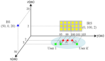
The simulation setup is shown in Fig. 3. It is assumed that BS, IRS (the central point), A1, A2 and A are located at (50, 0, 20), (0, 100, 2), (2, 99, 0), (2, 101, 0) and (2, 100, 0) in meter (m), respectively. We assume that the system operates on a carrier frequency of 750 MHz with the wavelength m and the path loss at the reference distance m is given by dB. Suppose that the IRS is equipped with a uniform planar array with 6 rows and 10 columns, and the element spacing is ; thus, we have . The noise power is set as 105 dBm. The channel from the BS to A1 is generated by , where denotes the distance from the BS to A1 and is the small-scale fading component. The same channel model is adopted for all other channels in general. Particularly, Rayleigh fading is assumed for the channels among the BS, IRS, A1, A2 and each User with the path loss exponents set as 3, whereas in the special channel case in Section IV, the channel between IRS and A is assumed to be LoS, with the path loss exponent set as 2. We also apply the scheme proposed in [13] for each of the users to estimate their channels consecutively, which serves as the benchmark.
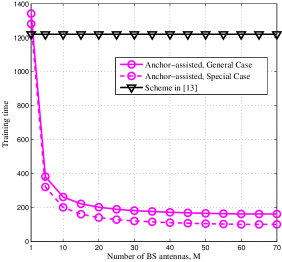
Fig. 4(a) shows the required training time (in terms of number of pilot symbols) versus the number of antennas, , at the BS. It is observed that as increases, the proposed scheme significantly reduce the training overhead as compared to that of the benchmark scheme (which is independent of ). This is because the proposed scheme exploits the multiple antennas at the BS for joint IRS channel estimation, whereas in the benchmark scheme the BS antennas estimate their associated channels independently in parallel. Note that when , the training overhead of the proposed scheme is even larger than that of the benchmark scheme. This is because additional pilot symbols are transmitted by anchors in Phase I, while the training efficiency in Phase II is not improved since in the case of . Moreover, it is observed that the proposed scheme under the special case of LoS IRS-anchor channel is more efficient as compared to the general channel case.
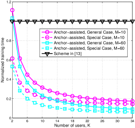
Fig. 4(b) shows the training time of the proposed scheme normalized by that of the benchmark scheme versus , with and 60, respectively. One can observe that the performance gap between the two schemes becomes larger as increases. This is because to accommodate one more user, the additional pilot overhead required by the benchmark scheme is , while that by the proposed scheme is . As a result, as increases, the pilot reduction by using the proposed scheme also increases. Also note that similar to Fig. 4(a), when is very small, the proposed scheme is even worse than the benchmark scheme. This reason is that additional / pilot symbols are required in Phase I, regardless of , while in the benchmark scheme, only pilot symbols are sufficient when .
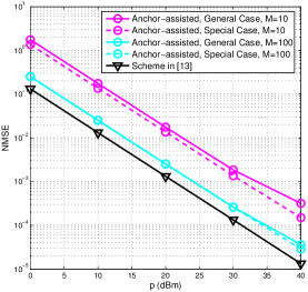
Fig. 4(c) shows the normalized mean-squared error (MSE) of the estimations of and versus the transmit power of pilot symbols in the on-line phase, with that of the off-line phase fixed as 40 dBm. It is observed that the MSE in the general channel case of the proposed scheme is highest, while that of the benchmark scheme is lowest. The reason is that although the proposed scheme significantly reduces the training overhead (see Figs. 4(a) and 4(b)), the estimation error in depends on both and . Specifically, in the general channel case, the error in comes from , and , while in the special channel case the error in comes from . In contrast, for the benchmark scheme, is estimated directly, which is thus less susceptible to noise/error. However, one can observe that the MSE of the proposed scheme is substantially reduced by increasing , and becomes even comparable when .
VI Conclusion
In this paper, we propose a new anchor-assisted channel estimation scheme for IRS-aided multiuser communications. By exploiting the fact that all BS-IRS-user cascaded channels share the same BS-IRS channel, the proposed scheme first estimates this common channel with only sign ambiguity via the anchor-assisted training. Then we show that the estimation of each cascaded BS-IRS-user channel is simplified to estimating each IRS-user channel with the number of unknowns significantly reduced from to , and the sign ambiguity in the estimated common channel does not affect the uniqueness of the recovered cascaded channels. Moreover, by exploring multi-antennas at the BS, the training overhead in estimating all users’ cascaded channels is reduced from to . Numerical results validate the effectiveness of the proposed scheme, especially when and/or is large. Considering the trend towards massive antenna arrays at the BS and massive connectivity with machine-type communications, our proposed scheme has the great potential of significantly improving the channel estimation efficiency in future IRS-aided wireless systems.
Appendix A
First, we show the following lemma.
Lemma 1: Given , can be estimated as , where , .
Proof: Because and , we have , which thus completes the proof.
Lemma 1 reveals that for given , there are rather than unknowns in and it can be rewritten as
Meanwhile, we can construct a candidate of as in Proposition 1, given by
| (24) |
Next, we consider the following two cases.
Case 1: . In this case, we have . Omitting the noise, we can express (18) as
| (25) |
Assuming that is full-rank, can be estimated as
| (26) |
Then, the cascaded BS-IRS-user channel is estimated as
| (27) |
Case 2: . Referring to (15), there must exist at least an such that . For illustration purpose, we assume that and for , while for all other possible ’s, the result can be similarly proved. Then we have
| (28) |
By omitting the noise, (18) can be written as
| (29) |
Accordingly, by using , is estimated as
| (30) |
Comparing in (28) with , we observe that the only difference lies in the sign of the elements in the first column and thus the following equality holds
| (31) |
Since we have
| (32) |
substituting (31) into (32) yields
| (33) |
Based on (30) and (33), the estimation of obtained by using can be written as
| (34) |
Though is not an exact estimation, the error only occurs in the sign of the first element of . Finally, the cascaded BS-IRS-user channel is recovered by
which is the same as (27).
Based on Cases 1 and 2, it is concluded that using constructed in Proposition 1 to estimate is always sufficient, regardless of whether is exactly the same as , which thus completes the proof of Proposition 1.
References
- [1] Q. Wu and R. Zhang, “Towards smart and reconfigurable environment: Intelligent reflecting surface aided wireless network,” IEEE Commun. Mag., vol. 58, no. 1, pp. 106-112, Jan. 2020.
- [2] S. Gong et al., “Towards smart radio environment for wireless communications via intelligent reflecting surfaces: A comprehensive survey,” 2019. [Online]. Available: https://arxiv.org/abs/1912.07794.
- [3] Q. Wu and R. Zhang, “Intelligent reflecting surface enhanced wireless network via joint active and passive beamforming,” IEEE Trans. Wireless Commun., vol. 18, no. 11, pp. 5394-5409, Nov. 2019.
- [4] B. Zheng, Q. Wu, and R. Zhang, “Intelligent reflecting surface-assisted multiple access with user pairing: NOMA or OMA?” IEEE Commun. Lett., vol. 24, no. 4, pp. 753-757, Apr. 2020.
- [5] Z. Ding and H. V. Poor, “A simple design of IRS-NOMA transmission,” IEEE Commun. Lett., vol. 24, no. 5, pp. 1119-1123, May 2020.
- [6] Q. Wu and R. Zhang, “Joint active and passive beamforming optimization for intelligent reflecting surface assisted SWIPT under QoS constraints,” IEEE J. Sel. Areas Commun., 2019, to appear. [Online]. Available: https://arxiv.org/abs/1910.06220.
- [7] C. Pan et al., “Intelligent reflecting surface enhanced MIMO broadcasting for simultaneous wireless information and power transfer,” 2019. [Online]. Available: http://arxiv.org/abs/1909.03272.
- [8] X. Guan, Q. Wu, and R. Zhang, “Intelligent reflecting surface assisted secrecy communication: Is artificial noise helpful or not?” IEEE Wireless Commun. Lett., Jan. 2020, DOI: 10.1109/LWC.2020.2969629.
- [9] H. Shen, W. Xu, S. Gong, Z. He, and C. Zhao, “Secrecy rate maximization for intelligent reflecting surface assisted multi-antenna communications,” IEEE Commun. Lett., vol. 23, no. 9, pp. 1488-1492, Sep. 2019.
- [10] Y. Yang, B. Zheng, S. Zhang, and R. Zhang, “Intelligent reflecting surface meets OFDM: Protocol design and rate maximization,” 2019. [Online]. Available: https://arxiv.org/abs/1906.09956.
- [11] D. Mishra and H. Johansson, “Channel estimation and low-complexity beamforming design for passive intelligent surface assisted MISO wireless energy transfer,” in Proc. IEEE ICASSP, May 2019.
- [12] C. You, B. Zheng, and R. Zhang, “Channel estimation and passive beamforming for intelligent reflecting surface: discrete phase shift and progressive refinement,” IEEE J. Sel. Areas Commun., 2019, to appear. [Online] Available: https://arxiv.org/abs/1912.10646.
- [13] B. Zheng and R. Zhang, “Intelligent reflecting surface enhanced OFDM: channel estimation and reflection optimization,” IEEE Wireless Commun. Lett., vol. 9, no. 4, pp. 518-522, Apr. 2020.