Analytical Study of the Non-Hermitian Semiclassical Rabi Model
Abstract
The symmetric semiclassical Rabi model explores the fundamental interaction between a two-level atom and a classical field, revealing novel phenomena in open systems through the inclusion of non-Hermitian terms. We propose a single similarity transformation that yields an effective Hamiltonian in rotating-wave approximation, enabling an analytical solution. The phase boundary of the -broken phase, derived from the analytical eigenvalues, closely matches the numerical exact one over a wide range of atomic frequencies, demonstrating the effectiveness of the analytical approach, especially at the main resonance. The Floquet parity operator is also introduced, providing a deeper physical understanding of the emergence of the -broken phase. Furthermore, by analyzing the dynamics of excited-state population, we observe several stable oscillations in the Fourier spectrum, demonstrating the applicability of the analytical method beyond the single-photon resonance region. The Bloch-Siegert shift is also discussed and, surprisingly, resembles its Hermitian counterpart, except for the higher-order terms in the coupling strength. The present analytical treatment provides a concise and accurate description of the main physics of this non-Hermitian atom-field interaction system.
I introduction
The Rabi model, describing the interaction between a two-level system and a classical driving field, is a cornerstone of quantum optics and atomic physics [1, 2, 3, 4, 5]. In recent years, there has been growing interest in extending the Rabi model to non-Hermitian systems, where the Hamiltonian is no longer self-adjoint [6, 7, 8, 9, 10, 11, 12]. The non-Hermitian systems, usually accompanied with complex eigenvalues, can exhibit rich and novel phenomena such as non-Hermitian phase transition [13, 14, 15], non-Hermitian quantum Hall effect [16, 17], non-reciprocal dynamics [18, 19], non-Hermitian quantum decoherence [20, 21], and so on. The non-Hermitian Hamiltonian provides a framework for investigating open systems and facilitates a deep understanding of the phenomena associated with non-Hermitian physics [22].
In particular, one of the most intriguing features of non-Hermitian systems is the concept of parity-time () symmetry, where the combined operation of parity (spatial inversion) and time-reversal symmetry allows for real eigenvalues even in the absence of Hermiticity [23, 24, 25, 26, 27]. When the system parameters cross certain critical values, the symmetry is broken, leading to the emergence of complex eigenvalues and the formation of exceptional points (EPs), where the eigenvalues and eigenstates coalesce [28]. The -symmetric non-Hermitian systems display numerous novel phenomena, such as -symmetric phase transition [29, 25], sensitivity enhancement [30, 31, 32], topological insulators [33, 34, 35, 36], and it thus offers some new physics which is absent in the Hermitian systems [37, 38, 39].
Although the time-independent non-Hermitian systems has been well developed, the question remains challenging when extended to time-dependent situations [40]. Several recent works have focused on time evolution and have uncovered a big amount of intriguing dynamical behaviors [41, 7, 8, 42, 43, 9, 44, 45, 11]. Some efforts have been made to investigate the nature of the non-Hermitian Rabi model (NHRM) [7, 8, 9, 46]. The NHRM can also be regarded as a periodically driven non-Hermitian two-level system [24]. The time-independent non-Hermitian two-level system [24] has been extensively studied in the literature and can be mapped to many important non-Hermitian systems. Hoverer, an exact analytical solution to the NHRM remains elusive, and the physical picture remains unclear. In this study, we aim to find a solvable analytical effective Hamiltonian and gain deeper understanding of the -symmetric NHRM.
The paper is structured as follows: In Sec. II, by using a similarity transformation, we transform the NHRM into the rotating-wave approximation (RWA) form with renormalized parameters, making the NHRM effectively solvable. In Sec. III, the analytical spectrum is obtained analytically from the effective solvable model. A comparison with the numerically exact results is performed. We introduce the Floquet parity operator and explain how the -broken phase emerges in Sec. IV. Section V is devoted to an analytical analysis of dynamics. The Fourier spectrum analysis is also presented in this section. The analytical Bloch-Siegert shift is presented and analyzed in Sec. VI. The last section contains some concluding remarks.
II Model and formalism
The Hamiltonian of the NHRM with the purely imaginary coupling strength [7] can be expressed as
| (1) |
where represents the atomic frequency, denotes the coupling strength between the atom and the external field, and stands for the field frequency. The operators represent the components of the Pauli matrix, where . Notably, this Hamiltonian exhibits symmetry, which can be demonstrated as
where the parity operator acts as , and the time-reversal operator transforms and . In the -unbroken phase, all quasi-energies are real, whereas in the -broken phase, the quasi-energies become complex.
In recent experiments, optical and radio-frequency fields provide an effective tool for manipulating atom loss, enabling the implementation of the NHRM Hamiltonian through time-periodic coupling between two spins in a dissipative system of ultracold atoms [46]. The two lowest hyperfine levels in a non-interacting Fermi gas of 6Li atoms are prepared. A resonant optical beam excites the atoms from the lower level to the excited state, generating atom loss in the lower level. This state-dependent, purely lossy system allows the lossy Hamiltonian to be mapped onto the -symmetric NHRM (1).
The structure of the phase diagram of the NHRM has been theoretically studied using perturbation theory [3], as discussed in Refs. [6, 7]. For the Hermitian semi-classical Rabi model, an analytically exact solution remains unavailable. However, some analytical studies based on perturbation theory [47] and unitary transformations [48, 49, 50] have been proposed, in addition to numerical solutions based on Floquet theory. For the NHRM, developing an accurate analytical scheme to bridge the gap between perturbation theory and the numerical exact solution would be valuable.
To facilitate the analytical study, we transform the above Hamiltonian in Eq. (1) into an effective RWA. Similar to the unitary transformation in the Hermitian semi-classical RM [48, 51], we introduce a similarity transformation with a generator in the present NHRM,
| (2) |
where is a coefficient to be determined later. We can then obtain the following transformed Hamiltonian
| (3) |
can be divided into three parts
| (4) | ||||
| (5) | ||||
| (6) |
where is the th-order Bessel function of the first kind, and the following identities have been used
| (7) | ||||
| (8) |
Note that is the time-independent component, while oscillates with a single-harmonic frequency. The term includes all higher-order harmonic terms and Bessel functions with orders . By neglecting , we can derive the effective Hamiltonian that retains only a single-harmonic frequency, which is .
At this point, the coefficient can be determined by solving the equation,
| (9) |
where is th-order modified Bessel function, and the identity has been used. The transformed Hamiltonian now takes an RWA-type form with a non-Hermitian coupling strength,
Applying a unitary transformation , we obtain a time-independent Hamiltonian as
| (10) |
where
Here, the renormalized atom characteristic frequency can be interpreted as an effective detuning, while the effective coupling strength is given by by Eq. (9). Thus, by performing a single similarity transformation and neglecting higher-order harmonic terms, we derive an effective non-Hermitian two-level atomic Hamiltonian, which forms the foundation of our subsequent work.
III phase diagram and quasi-eigenvalues spectrum
An essential characteristic of -symmetric models is their spectrum. Despite the non-Hermitian nature of the Hamiltonian, all eigenvalues become real under certain parameter conditions. We designate the system as being in a -unbroken phase when these parameters guarantee real eigenvalues. Conversely, when the parameters result in the appearance of imaginary parts in the eigenvalues, we characterize the system as being in a -broken phase.
In the time-periodic model, the eigenvalues of the instantaneous Hamiltonian do not have the same physical meaning as those in time-independent scenarios. Therefore, we must study the quasi-eigenvalues. Fortunately, we derived a solvable effective time-independent Hamiltonian in Eq. (10) in the previous section, allowing us to readily obtain its eigenvalues.
| (11) |
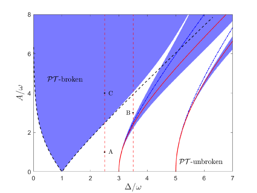
The exceptional points are given by , as derived from Eq. (11), which directly yield the phase diagram directly in Fig. 1. When , the model is in a -unbroken phase, characterized by real eigenvalues. Conversely, when , the eigenvalues become complex and conjugate in pairs. The black dashed line in Fig. 1 separates the two phases, which are just the EPs.
To solve the time-periodic NHRM numerically, we apply Floquet theory to obtain the quasi-eigenvalues. For the NHRM Hamiltonian (1), the Floquet Hamiltonian is given by . As detailed in Appendix A, we perform exact diagonalization (ED) on the matrix form of the Floquet Hamiltonian. Using the numerically obtained quasi-eigenvalues, we determine the boundary between the -broken and -unbroken phases, as shown in Fig. 1, marked by the blue-shaded region.
Interestingly, the present analytical phase boundary (black dashed lines) agrees excellently with with the exact numerical results over a wide atomic frequency range, up to (the three-photon resonance), which constitutes the primary region for the -broken phase. When , additional -broken phases intervene the -unbroken region. These secondary -broken phases, however, are not captured by the current analytical scheme. Is the present analytical scheme unable to provide any information about the secondary -broken phases? The answer is ”no”.
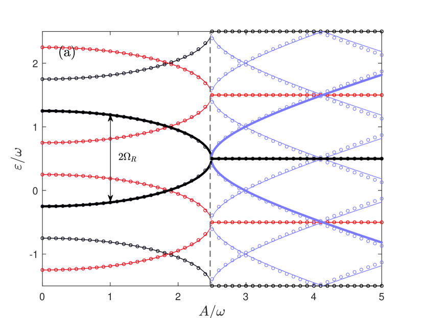
We present the eigenvalues from both the analytical scheme ( Eq. (11), open circles) and the Floquet theory (thick curves) in Fig. 2 for and . These two values are marked by two vertical red dashed lines in Fig. 1, both cross the primary -broken phase boundary, but line also crosses the secondary -broken phase boundary. According to the Floquet theorem, for a time-periodic Hamiltonian, the quasi-eigenvalues shifted by ( is an integer) do not change the physical state, similar to a generalized Brillouin zone in the Bloch band theory. For later reference, we also display some shifted quasi-eigenvalues for both the analytical scheme (Eq. (11)) and Floquet theory.
Figure 2 (a) shows that the analytical results closely agree with the numerical quasi-energies for the coupling strengths up to for . The analytical EPs, indicated by dashed lines, are nearly identical to the numerical ones.
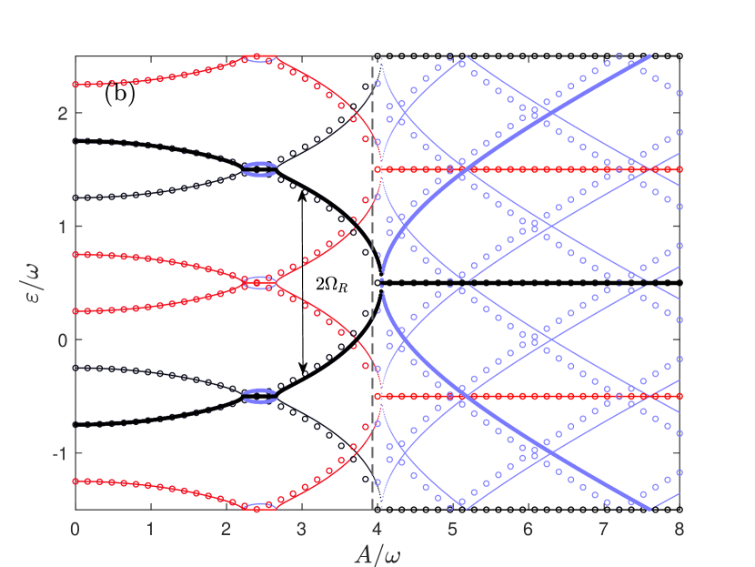
As shown in Fig. 2 (b) for, the analytical quasi-eigenvalues agree with the numerical results, except in the small, ellipse-shaped region around quasi-eigenvalues . In this region, the analytical scheme can only provide real quasi-eigenvalues, and level crossings occur, while the numerical results yield complex quasi-eigenvalues. Further analysis will be presented in the next section to explain these observations, based on the uncovered symmetry of the NHRM within the framework of Floquet theory.
IV Floquet parity operator and spectrum analysis
To explain the -symmetry breaking and the EPs discussed in the previous section, we introduce the Floquet parity operator
where is constructed using the state vector from an orthonormal, complete Fourier basis set in the Hilbert space of -periodic function. It can be shown that , where is the Floquet Hamiltonian. This implies that the Hilbert space of the Floquet Hamiltonian can be decomposed into two independent subspaces, corresponding to even and odd Floquet parity, with eigenvalues , respectively.
For odd (even) parity (), the subspace basis should be , so that the Floquet Hamiltonian can be expressed as
| (12) |
We can also numerically diagonalize this matrix for both even and odd parity to calculate the corresponding quasi-eigenvalues.
The quasi-eigenvalues, denoted by the thick curves in Fig. 2, correspond to the odd parity subspace. Quasi-eigenvalues shifted by , marked in black, also belong to this subspace. In contrast, the quasi-eigenvalues of even parity are shifted by , as marked in red. In principle, quasi-eigenvalues with different parities may cross. However, within the same parity subspace, they cannot intersect without an additional symmetry. Fortunately the present NHRM just possesses an alternative symmetry, which enables quasi-eigenvalues within the same parity subspace to intersect, leading to EPs. This phenomenon underlies the symmetry breaking and the emergence of EPs.
The picture above illustrating the symmetry breaking fully describes the features of the quasi-eigenvalue spectrum shown in Fig. 2. Two branches of the thick curve (representing real values), both with the same odd parity, approach each other as increases and intersect at the vertical dashed line, forming the primary EPs. These EPs can be accurately captured by in Eq. (11).
As mentioned above, the eigenvalue , shifted by , retains the same parity. If the shifted cross with , i.e., , then we have
| (13) |
This equation gives the coupling strength for a given , at which the real eigenvalues cross, thus corresponding to the -broken region. The primary EP corresponds to in this equation. We can also determine the crossing points where real eigenvalues with the same parity intersect, for any .
The lines representing the crossing points for and are shown as red solid lines in Fig. 1, both lying within the -broken region. Using perturbation theory, Lee et al. predicted a line of maximal symmetry breaking (where the imaginary eigenvalue is maximized) in Ref. [7], shown as a blue dash-dotted line in Fig.1 for comparison. The two lines agree well for small but begin to deviate as increases. Noticeably, their line for does not lie within the -broken region, while ours does. Therefore, our analytical scheme can more accurately predict the onset of symmetry breaking, beyond the primary -broken phase, particularly when exceeds .
If is very small, and higher-order terms in are neglected, we can derive a closed-form solution to Eq. (13),
| (14) |
Based on the similarity transformation in Sec. II, this result is exact in the limit as . Since , the crossing point occurs at . This indicates that the -broken line intersect the axis at these resonance points.
As shown in Fig. 1 and in Ref. [7], the second and third -broken phases, for and , are expected to be extremely narrow at small values of near 0, but they do not extend to the axis according to numerical calculations. This discrepancy arises from the numerical calculations, which require truncation, while the exact solution can only be obtained using an infinite basis. At the single-photon resonance for , Eq. (14) gives , consistent with the primary -broken region, which touches axis at , as shown in Fig. 1.
We now focus on the more complicated Floquet quasi-eigenvalues spectrum in Fig. 2 (b) for . Specifically, within the small, ellipse-shaped region around quasi-eigenvalues , the present analytical results from Eq. (11), denoted by the open circles, show real level crossings. The crossing point at can be calculated from Eq. (13) for . This is also the point where the first red solid line intersects the second vertical red dashed line in Fig.1. However, the two real quasi-eigenvalues with the same parity cannot cross. As a result, an imaginary part emerges to resolve this issue, signaling the new PT symmetry breaking. The analytical results in Eq. (11) cannot fully describe, but can predict this -broken region. In contrast, real spectrum lines with different parities can cross at .
When , i.e. -photon resonance, the two quasi-eigenvalues with the same parity coincide at , as proven in Eq. (14) for any . If increases slightly, the two quasi-eigenvalues will intersect. However, they cannot cross because they share the same parity. As a result, a complex quasi-eigenvalue must emerge to prevent the crossing of real quasi-eigenvalues, leading to the formation of EP points.
If , as demonstrated in Fig. 2 (b), the two adjacent quasi-eigenvalues obtained from the numerical diagonalization of the matrix (12), which share the same parity (both black or both red lines), should avoid crossing each other at a finite value of . Consequently, a -broken phase emerges, indicated by small, ellipse-shaped blue curves representing the imaginary part of the quasi-eigenvalues. This explains the origin of the second -broken region in Fig. 1. However, two adjacent real quasi-eigenvalues from the analytical scheme cross in the -broken region. In other words, the analytical scheme cannot fully describe this -broken region, but can predict its location. If we further increase to the range , both adjacent and next-adjacent numerical quasi-eigenvalues avoid the real quasi-eigenvalue crossing. Consequently, two -broken phases emerge, as illustrated in Fig. 1 by the second and third -broken regions. At large , the widths of the different -broken regions can become large enough to merge into a single, contiguous -broken region.
So far, we have explained the origin of the -broken phases and accounted for the phase diagram using the conserved Floquet parity operator. Additionally, the Floquet parity operator can be applied to the Hermitian semi-classical Rabi model. Within the same parity subspace, real quasi-energies cannot cross but instead exhibit an avoided-crossing feature [3]. As shown in Appendix A, quasi-energies with different parities can cross, whereas quasi-energies with the same parity can only avoid each other. The present non-Hermitian model exhibits richer and more complex properties than its Hermitian counterpart, due to the additional symmetry.
Our current analytical scheme, based on a single similarity transformation, accurately describes the phase diagram for and can also predict the new -broken region at . By combining the primary -broken region for , determined by Eq. (11), with the -broken line from Eq. (13) for , as shown in Fig. 1, our analytical scheme can produce a highly accurate, nearly exact phase diagram within for arbitrary , except for the small region of the second -broken phase. In the next section, we will examine whether it accurately captures the dynamics.
V Dynamics of the two-level system
In this section, We explore the time-evolution of the two-level system. The time dependent wavefunction can be represented as , where and denote the probability amplitudes of the upper and lower states, respectively, in a two-level atom. Using the Schrödinger equation, we can derive the following two coupled first-order differential equations:
| (15) | ||||
| (16) |
The exact dynamics can be determined by numerically solving two coupled dynamical equations, as an analytical solution is highly challenging. An effective approximation involves applying the RWA to decouple the probability amplitudes. This approach simplifies the calculation and provides the population evolution of the excited state as
| (17) |
where . The population grows exponentially when is imaginary and can exceed unity due to the non-conservation of probability in non-Hermitian systems.
The above quasi-eigenvalues in Eq. (11) allow us to analytically study the dynamical properties of the NHRM. Using the similarity transformation (2) and the unitary transformation , we can define the time evolution operator as
| (18) |
by which we can derive analytically the time-dependent wavefunction starting from an initial state . The time evolution operator in Eq. (18) applies a sequence of transformations to the initial state, moving it to a new gauge. The state evolves under the time-independent Hamiltonian until time . Finally, we arrive at the evolved state to the original frame using the transformation , yielding the final state .
The atom is initially prepared in the ground state, so . In our analysis, we focus on the atomic population of the excited state, denoted as , representing the probability of finding the atom in its excited state at time . This initial state has a definite parity, so its evolution involves only eigenstates in the same parity subspace. The analytical result can be written as:
| (19) |
where
Here, is the Rabi frequency from Eq. (11). measures the gap between the two branches of the quasi-eigenvalues for the same in the eigenvalue spectrum, as illustrated in Fig. 2 (b) by the black double arrow connecting the open circles. Adjacent quasi-eigenvalues with the same parity are shifted by . The quasi-eigenvalue differences dominating the dynamics can include , , as well as other combinations and multiples of and .
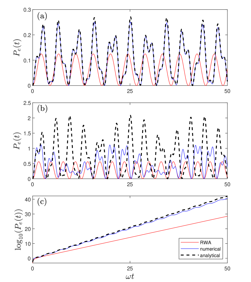
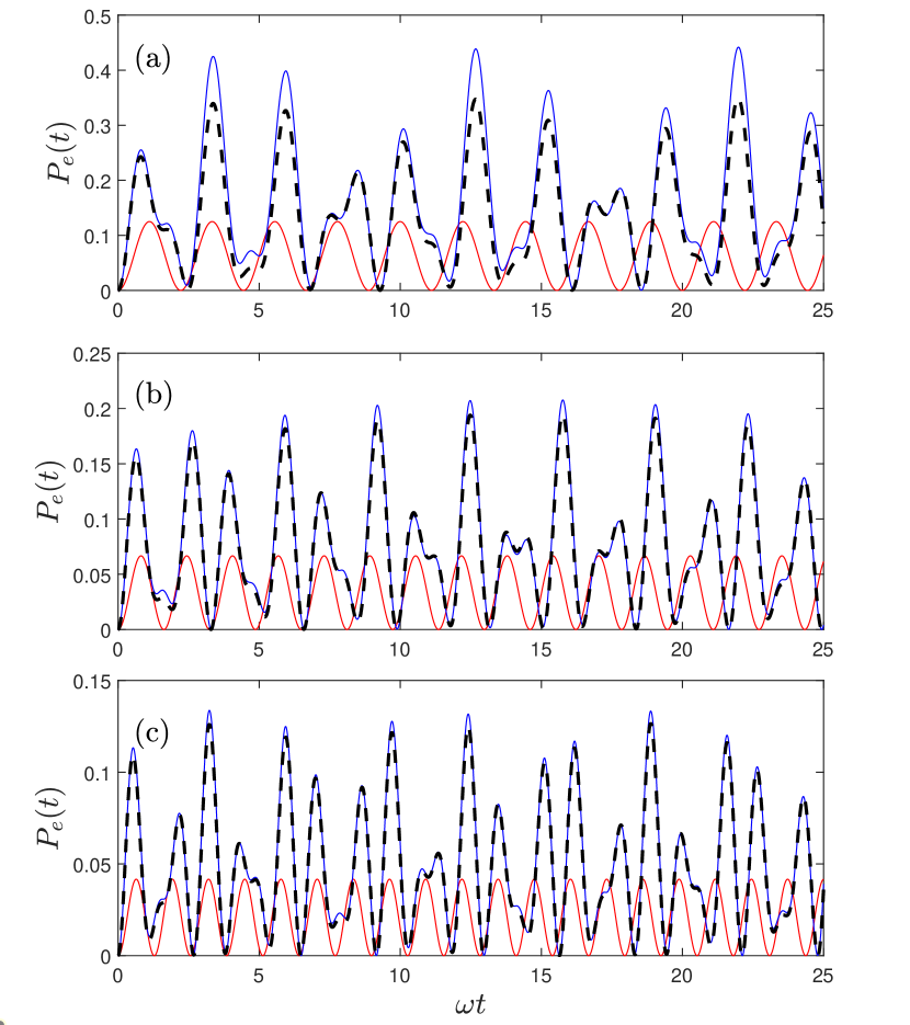
In Fig. 3, we show the time evolution of the atom at three representative points: A (, ), B (, ), and C (, ). These points lie in different regions of the phase diagram in Fig. 1, and we analyze them using the present analytical approach (19), numerical simulations, and the RWA (17). As illustrated in Fig. 3 (c), at point C in the -broken phase, dominated by single-photon resonance, the population in the excited state grows roughly exponentially, eventually surpassing unity. This feature is fully described by Eq. (19). This intriguing emergent phenomenon has significant implications for non-Hermitian dynamics. Unlike Hermitian systems, our model equivalently treats open systems, leading to a breakdown in probability conservation. Interestingly, the present analytical results for population evolution perfectly agree with the numerical results. The RWA can only accurately describe population evolution in the short-time regime. While the RWA can predict the dominant exponential behavior (cf. Eq. (17)), it underestimates the growth rate. Additionally, we find that the RWA yields a smoothed evolution without the oscillatory feature due to the neglect of counter-rotating terms.
In the -unbroken phase, represented in Fig. 3 (a) and (b), stable oscillations with multiple frequencies and varying amplitudes are observed, in contrast to the -broken phase, where exponential dynamics dominate. The present analytical results, given by Eq. (19), perfectly describe these oscillations at point A for . At point B, the analytical results match the exact dynamics only at the very early stage and deviate significantly throughout the rest of the process. Nevertheless, they qualitatively capture the multi-oscillation feature, including oscillations with multiple frequencies.
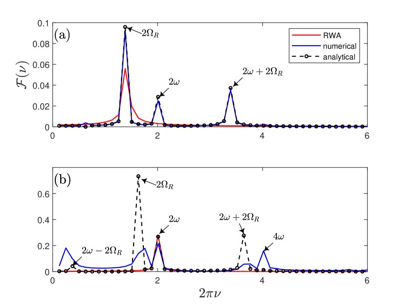
To analyze the dynamics and stable oscillations in the -unbroken phase in greater detail, we perform a Fourier spectral analysis of the population time evolution. The Fourier transform, a fundamental technique for frequency decomposition, is defined as follows:
where represents the spectrum as a function of frequency , and denotes the observed time evolution as a function of time .
The frequency spectrum of the atomic population time evolution is shown in Fig. 4. At the point A, as shown in Fig. 4 (a), the numerical frequency spectrum exhibits three peaks, precisely corresponding to , , and , all these three frequencies measure the gaps between the two quasi-eigenvalues within the same parity in the analytical scheme. These frequencies also correspond to the lowest three frequencies in Eq. (19), further demonstrating that our analytical method accurately describes the time evolution in the -unbroken phase for .
As shown in Fig. 4 (b) for point B, the exact frequency spectrum exhibits five peaks, while our analytical results yield four main peaks, missing only the last one. The analytical frequency peaks are marked with arrows, indicating the differences between two quasi-eigenvalues of the same parity. In both Fig. 4 (a) and (b), the main peaks corresponding to , , and also appear in the exact dynamics. In panel (b), however, the additional peaks around and in the numerically exact dynamics are only weakly captured in the analytical results. At point B, the atomic frequency lies beyond the three-photon resonance region, so additional higher-order frequency terms are required. Therefore, to obtain a more precise description, additional similarity transformations should be added in Eq. (2). For qualitative studies, the current analytical scheme, which uses a single similarity transformation, can capture the main features of the dynamics.
We have also extensively examine the dynamics for large atomic frequencies , in the -unbroken phase, as demonstrated in Appendix B. Our analytical results agree well with the exact ones as long as the coupling strength is not too strong. The RWA can only provide the primary oscillation frequency, known as the Rabi frequency, and thus cannot fully capture the complex features of the time evolution, as shown in Figs. 3, 4, and 7. The RWA Rabi frequency also deviates from the exact values at strong coupling, whereas the analytical Rabi frequency agrees well with the exact values in all cases.
VI Bloch-Siegert shift
In this section, we will discuss the Bloch-Siegert (BS) shift in the NHRM, which is a key issue in its Hermitian counterpart [3, 49, 52].
In the Hermitian system, the BS shift represents the offset of the resonance frequency from the original driven frequency, i.e., . The resonance frequency is determined by the maximum time-averaged transition probability, corresponding to the largest oscillation amplitude. However, in the non-Hermitian system, when the frequency reaches resonance, the probability diverges rapidly. In this case, the quasienergies exhibit the largest imaginary component. The condition of the resonance is
| (20) |
where can be obtained from Eq. (9) as
Solving Eq. (20) yields , allowing us to compute the BS shift in the present analytical scheme.
A simple analytical expression for the BS shift, expanded in powers of the coupling strength , can also be derived. In this process, we expand and up to the fourth order in ,
Using Eq. (9), we expand the coefficient up to second order in ,
The minus sign in the second term arises from the imaginary coupling , which changes the sign in the Hermitian counterpart [48]. Therefore, the modulated Rabi frequency, up to fourth order in , is given by
| (21) |
We can now obtain the resonance frequency,
| (22) |
Note that the term is consistent with the one found in perturbation theory [7]. Additionally, by applying the concise similarity transformation method, we can derive the higher-order solution for the BS shift.
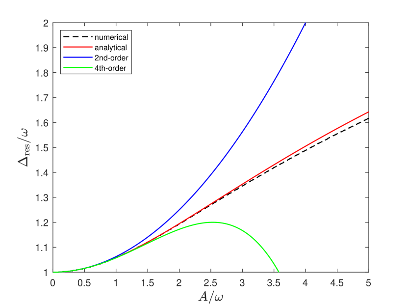
The analytical BS shift, based on Eq. (20), is shown by the red line in Fig. 5 . Interestingly, our results match the numerical data very well across a wide range of coupling strengths, up to . Note that the perturbation result for the BS in Ref. [7], marked in blue, begins to deviate from the exact values at . Surprisingly, the presence of the -broken phase in this non-Hermitian model does not significantly affect the BS shift across a broad range of coupling strengths, even when passing through multi-photon resonance. This may be due to the fact that the BS shift can be expressed as a function of .
VII conclusion
This work studies the NHRM analytically. First, we derive a transformed NHRM in the RWA form using a single similarity transformation. Next, we obtain an effective Hamiltonian for the non-Hermitian two-level system by applying a rotating operation, which explicitly yields two eigenvalues and an EP. Thus, the quasi-eigenvalues can thus be obtained from the two eigenvalues by shifting them by a multiple of the field frequency. The exact quasi-eigenvalues can be determined numerically using Floquet theory. Notably, our analytical results for the quasi-eigenvalues agree excellently with the numerical results in the single-photon resonance regime. The primary -broken phase boundary is also detected in a wide parameter regime, extending even beyond the multi-photon resonance region.
We also uncover a Floquet parity symmetry that commutes with the Floquet Hamiltonian of the NHRM. The conserved parity decomposes the entire Floquet space into two subspaces with different parity. The quasi-eigenvalues are associated with one of two parities. Quasi-eigenvalues shifted by even multiples of the field frequency, , belong to the same parity. When the atomic frequency exceeds an odd multiple of the field frequency, i.e., , two adjacent quasi-eigenvalues within the same parity will intersect. However, they cannot truly cross without an additional symmetry. Therefore, a complex quasi-eigenvalue emerges to resolve this issue, leading to the secondary -broken phase. Interestingly, in this region, our analytical real quasi-eigenvalues cross, predicting the -broken location, though it cannot describe the -broken.
The dynamics are also investigated within the analytical scheme. In the single-photon resonance regime, i.e., , the time evolution of the atomic population, starting from the atomic upper state, as predicted by the analytical scheme, closely matches the numerical results. Even in the higher-photon resonance regime, Fourier transform analysis shows that the analytical scheme can captures multi-oscillations, with the dominant frequencies aligning with those observed in the exact dynamics. Additionally, the BS shift, as derived analytically in the present scheme, agrees well with the exact result over a wide coupling regime. This further highlights that the simple analytical scheme effectively captures the main features of this non-Hermitian qubit-cavity coupling model.
To accurately describe the secondary -broken phase and dynamics in higher-order resonance regimes, additional similarity transformations are required. The research along this direction is in progressing. The proposed analytical method for the NHRM may offers a valuable alternative for exploring open systems and atom-field interactions. Its versatility extends to more complex models, including those with multiple cavity frequencies, higher-order interactions, or additional qubits.
Acknowledgements.
This work is supported by the National Key RD Program of China (Grant No. 2024YFA1408900) and the National Natural Science Foundation of China (Grant No. 12305032).Appendix A: Numerical method for quasi-energy spectrum

In this Appendix, we provide a brief description of the Floquet picture for the NHRM. A complete set of orthonormal basis states of space can be constructed by combining a complete set of orthogonal and normalized basis states of , , with the complete set of time-periodic functions labeled by the integer ,
Using the definition of the scalar product in the extended Floquet Hilbert space, the matrix elements can be obtained of the Floquet Hamiltonian with respect to the basis ,
| (23) |
where
In the matrix form, the Floquet Hamiltonian can be expressed as
| (24) |
The quasi-eigenvalues are the eigenvalues of this infinite matrix. The exact numerical diagonalization of the matrix (24) is performed using a large truncated space.
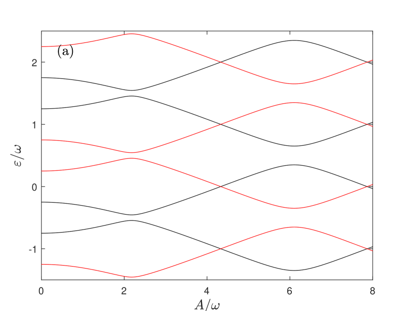
For comparison, we calculate the Floquet quasi-energies for the Hermitian counterpart using the same model parameters as in Fig. 2. The results are presented in Fig. 6. In the time-periodic Hermitian model, quasi-energies with the same parity exhibit only the avoided-crossing feature, in contrast to its non-Hermitian counterpart. Quasi-energies with different parities can cross. This is consistent with the Floquet parity symmetry.
Appendix B: Dynamics of more parameters
We can examine the dynamics using our analytic approach in -unbroken phase over a broader parameter regime. As shown in Fig. 7, we compare the dynamics for the different atomic frequencies: (a) , (b) , and (c) , all at the same coupling strength . We observe that the population of the excited state maintains stable oscillations, and our analytical method matches remarkably well with the numerical results.
As shown in Fig. 7 (c), even when the atomic frequency lies above the higher-order -broken regions, such as the five-photon resonance region, our analytical approach still accurately captures the dynamic behavior. This suggests that our analytic method is available for a wide range of coupling strengths and arbitrary atomic frequencies. Interestingly, as the frequency of atoms increases, the analytical results align more closely with the numerical ones.
References
- Rabi [1936] I. I. Rabi, Phys. Rev. 49, 324 (1936).
- Rabi [1937] I. I. Rabi, Phys. Rev. 51, 652 (1937).
- Shirley [1965] J. H. Shirley, Phys. Rev. 138, B979 (1965).
- Braak et al. [2016] D. Braak, Q.-H. Chen, M. T. Batchelor, and E. Solano, J. Phys. A: Math. Theor. 49, 300301 (2016).
- Gerry and Knight [2023] C. C. Gerry and P. L. Knight, Introductory quantum optics (Cambridge university press, 2023).
- Joglekar et al. [2014] Y. N. Joglekar, R. Marathe, P. Durganandini, and R. K. Pathak, Phys. Rev. A 90, 040101 (2014).
- Lee and Joglekar [2015] T. E. Lee and Y. N. Joglekar, Phys. Rev. A 92, 042103 (2015).
- Gong and Wang [2015] J. Gong and Q.-h. Wang, Phys. Rev. A 91, 042135 (2015).
- Xie et al. [2018] Q. Xie, S. Rong, and X. Liu, Phys. Rev. A 98, 052122 (2018).
- Quijandría et al. [2018] F. Quijandría, U. Naether, S. K. Özdemir, F. Nori, and D. Zueco, Phys. Rev. A 97, 053846 (2018).
- Wang et al. [2021] H. Wang, X. Zhang, J. Hua, D. Lei, M. Lu, and Y. Chen, Journal of Optics 23, 123001 (2021).
- Lu et al. [2023] X. Lu, H. Li, J.-K. Shi, L.-B. Fan, V. Mangazeev, Z.-M. Li, and M. T. Batchelor, Phys. Rev. A 108, 053712 (2023).
- Wei and Jin [2017] B.-B. Wei and L. Jin, Sci. Rep. 7, 7165 (2017).
- Longhi [2019] S. Longhi, Phys. Rev. Lett. 122, 237601 (2019).
- Öztürk et al. [2021] F. E. Öztürk, T. Lappe, G. Hellmann, J. Schmitt, J. Klaers, F. Vewinger, J. Kroha, and M. Weitz, Science 372, 88 (2021).
- Yoshida et al. [2019] T. Yoshida, K. Kudo, and Y. Hatsugai, Sci. Rep. 9, 16895 (2019).
- Ochkan et al. [2024] K. Ochkan, R. Chaturvedi, V. Könye, L. Veyrat, R. Giraud, D. Mailly, A. Cavanna, U. Gennser, E. M. Hankiewicz, B. Büchner, et al., Nat. Phys. 20, 395 (2024).
- Reisenbauer et al. [2024] M. Reisenbauer, H. Rudolph, L. Egyed, K. Hornberger, A. V. Zasedatelev, M. Abuzarli, B. A. Stickler, and U. Delić, Nat. Phys. 20, 1629 (2024).
- Brighi and Nunnenkamp [2024] P. Brighi and A. Nunnenkamp, Phys. Rev. A 110, L020201 (2024).
- Castagnino and Fortin [2012] M. Castagnino and S. Fortin, J. Phys. A: Math. Theor. 45, 444009 (2012).
- Dey et al. [2019] S. Dey, A. Raj, and S. K. Goyal, Phys. Lett. A 383, 125931 (2019).
- Yuto Ashida and Ueda [2020] Z. G. Yuto Ashida and M. Ueda, Adv. Phys. 69, 249 (2020).
- Leggett et al. [1987] A. J. Leggett, S. Chakravarty, A. T. Dorsey, M. P. A. Fisher, A. Garg, and W. Zwerger, Rev. Mod. Phys. 59, 1 (1987).
- Bender and Boettcher [1998] C. M. Bender and S. Boettcher, Phys. Rev. Lett. 80, 5243 (1998).
- Konotop et al. [2016] V. V. Konotop, J. Yang, and D. A. Zezyulin, Rev. Mod. Phys. 88, 035002 (2016).
- El-Ganainy et al. [2018] R. El-Ganainy, K. G. Makris, M. Khajavikhan, Z. H. Musslimani, S. Rotter, and D. N. Christodoulides, Nat. Phys. 14, 11 (2018).
- Bender [2023] C. M. Bender, in TIME AND SCIENCE: Volume 3: Physical Sciences and Cosmology (World Scientific, 2023) pp. 285–310.
- Moiseyev [2011] N. Moiseyev, Non-Hermitian quantum mechanics (Cambridge University Press, 2011).
- Bender et al. [2013] C. M. Bender, B. K. Berntson, D. Parker, and E. Samuel, American Journal of Physics 81, 173 (2013).
- Liu et al. [2016] Z.-P. Liu, J. Zhang, i. m. c. K. Özdemir, B. Peng, H. Jing, X.-Y. Lü, C.-W. Li, L. Yang, F. Nori, and Y.-x. Liu, Phys. Rev. Lett. 117, 110802 (2016).
- Li et al. [2016] J. Li, R. Yu, C. Ding, and Y. Wu, Phys. Rev. A 93, 023814 (2016).
- Farhat et al. [2020] M. Farhat, M. Yang, Z. Ye, and P.-Y. Chen, ACS Photonics 7, 2080 (2020).
- Hu and Hughes [2011] Y. C. Hu and T. L. Hughes, Phys. Rev. B 84, 153101 (2011).
- Ni et al. [2018] X. Ni, D. Smirnova, A. Poddubny, D. Leykam, Y. Chong, and A. B. Khanikaev, Phys. Rev. B 98, 165129 (2018).
- Ezawa [2021] M. Ezawa, Phys. Rev. Res. 3, 043006 (2021).
- Fritzsche et al. [2024] A. Fritzsche, T. Biesenthal, L. J. Maczewsky, K. Becker, M. Ehrhardt, M. Heinrich, R. Thomale, Y. N. Joglekar, and A. Szameit, Nat. Mater. 23, 377 (2024).
- Guo et al. [2009] A. Guo, G. J. Salamo, D. Duchesne, R. Morandotti, M. Volatier-Ravat, V. Aimez, G. A. Siviloglou, and D. N. Christodoulides, Phys. Rev. Lett. 103, 093902 (2009).
- Feng et al. [2017] L. Feng, R. El-Ganainy, and L. Ge, Nat. Photonics 11, 752 (2017).
- Kawabata et al. [2019] K. Kawabata, K. Shiozaki, M. Ueda, and M. Sato, Phys. Rev. X 9, 041015 (2019).
- Fring and Frith [2017] A. Fring and T. Frith, Phys. Rev. A 95, 010102 (2017).
- Luo et al. [2013] X. Luo, J. Huang, H. Zhong, X. Qin, Q. Xie, Y. S. Kivshar, and C. Lee, Phys. Rev. Lett. 110, 243902 (2013).
- Doppler et al. [2016] J. Doppler, A. A. Mailybaev, J. Böhm, U. Kuhl, A. Girschik, F. Libisch, T. J. Milburn, P. Rabl, N. Moiseyev, and S. Rotter, Nature 537, 76 (2016).
- Hassan et al. [2017] A. U. Hassan, B. Zhen, M. Soljačić, M. Khajavikhan, and D. N. Christodoulides, Phys. Rev. Lett. 118, 093002 (2017).
- Koutserimpas et al. [2018] T. T. Koutserimpas, A. Alù, and R. Fleury, Phys. Rev. A 97, 013839 (2018).
- Zhang et al. [2019] D.-J. Zhang, Q.-h. Wang, and J. Gong, Phys. Rev. A 100, 062121 (2019).
- Li et al. [2019] J. Li, A. K. Harter, J. Liu, L. de Melo, Y. N. Joglekar, and L. Luo, Nat. Commun. 10, 855 (2019).
- Hausinger [2010] J. Hausinger, Phys. Rev. A 81 (2010).
- Lü and Zheng [2012] Z. Lü and H. Zheng, Phys. Rev. A 86, 023831 (2012).
- Yan et al. [2015] Y. Yan, Z. Lü, and H. Zheng, Phys. Rev. A 91, 053834 (2015).
- Han et al. [2024] Y. Han, S. Zhang, M. Zhang, Q. Guan, W. Zhang, and W. Li, Phys. Rev. A 109, 053704 (2024).
- Twyeffort Irish and Armour [2022] E. K. Twyeffort Irish and A. D. Armour, Phys. Rev. Lett. 129, 183603 (2022).
- Bloch and Siegert [1940] F. Bloch and A. Siegert, Phys. Rev. 57, 522 (1940).