Analytical solution for an acoustic boundary layer around an oscillating rigid sphere
Abstract
Analytical solutions in fluid dynamics can be used to elucidate the physics of complex flows and to serve as test cases for numerical models. In this work, we present the analytical solution for the acoustic boundary layer that develops around a rigid sphere executing small amplitude harmonic rectilinear motion in a compressible fluid. The mathematical framework that describes the primary flow is identical to that of wave propagation in linearly elastic solids, the difference being the appearance of complex instead of real valued wave numbers. The solution reverts to well-known classical solutions in special limits: the potential flow solution in the thin boundary layer limit, the oscillatory flat plate solution in the limit of large sphere radius and the Stokes flow solutions in the incompressible limit of infinite sound speed. As a companion analytical result, the steady second order acoustic streaming flow is obtained. This streaming flow is driven by the Reynolds stress tensor that arises from the axisymmetric first order primary flow around such a rigid sphere. These results are obtained with a linearization of the non-linear Navier-Stokes equations valid for small amplitude oscillations of the sphere. The streaming flow obeys a time-averaged Stokes equation with a body force given by the Nyborg model in which the above mentioned primary flow in a compressible Newtonian fluid is used to estimate the time-averaged body force. Numerical results are presented to explore different regimes of the complex transverse and longitudinal wave numbers that characterize the primary flow.
I Introduction
Acoustic streaming is the steady flow generated by periodic small amplitude Rayleigh acoustic fields in compressible Newtonian fluids. In certain flow regimes, the streaming patterns are observed as intricate steady vortices or circulatory patterns near solid boundaries. The creation of a steady streaming flow due to a periodic acoustic wave is inherently a non-linear effect that arises from the time averaged velocity field governed by the time-dependent Navier-Stokes equations. The role of fluid viscosity and the generation of vorticity near solid boundaries are key to the streaming phenomenon so that details of such flow depend on the geometry of the system and on the hydrodynamic boundary conditions. Consequently, the flow characteristics will vary near solid or soft surfaces such as biological cell membranes, bubble surfaces or fluid interfaces and as such can provide very different modes of steady fluid transport. Recent advances in microfluidics and ultrasonic technologies stimulated resurgent interest in these phenomena [1, 2, 3, 4, 5, 6, 7, 8].
From the point of view of analytical and numerical analysis, acoustic streaming has also attracted renewed interest recently, for example around spheres, bubbles and drops [9, 10], including thermal effects [11, 12]. Previous studies of steady streaming around a stationary sphere considered an imposed external oscillatory flow field [13, 14], or streaming around bubbles and drops [15, 16]. The amplitude of the oscillations is also assumed to be small compared to the sphere radius. As the fluid is generally taken to be incompressible this is termed steady streaming rather than acoustic streaming [17]. Streaming around a stationary sphere in a compressible fluid has been considered by Lee and Wang [18]. However, they made a further assumption to only consider the flow outside the boundary layer to simplify the analysis.
To elucidate the physics of such complex flows, it is instructive to have available analytical solutions for special cases that can also serve as test cases for more complex numerical models. It turns out that the governing equations and boundary conditions for an oscillating rigid sphere in an infinite but otherwise quiescent compressible Newtonian fluid is very similar to a rigid sphere undergoing oscillatory motion in an infinite linear elastic material for which a analytical solution has been given recently by Klaseboer et al. [19].
This oscillatory motion of a sphere in a compressible Newtonian fluid generates both an acoustic field due to compressibility of the fluid and an acoustic boundary layer in the fluid near the sphere due to viscosity. Without further approximations, we can construct an analytic solution that accounts for the transition from viscous boundary layer dominated flow near interfaces to near potential flow far from boundaries. The known limits of negligible viscosity, negligible compressiblity or zero frequency can be recovered as special cases. In the geometric limit of a large sphere, results for both normal and tangential flows at a planar surface are obtained at different parts of the sphere. To the best knowledge of the authors, such a theoretical solution has not appeared in the literature before. Taking this analytical solution to be the primary solution, we then obtain an expression for the secondary flow or acoustic streaming that originates from small non-linear inertial effects.
At low amplitudes of oscillation [20], the streaming flow can be obtained as a non-linear steady secondary correction to the linear time-dependent primary flow. In this paper, we present a general analytic solution of the model [21] for streaming flow in a compressible Newtonian fluid around a rigid sphere with radius, that is executing rectilinear oscillatory motion with angular frequency, and velocity amplitude, . We focus on the Rayleigh [22] or acoustic limit in which the magnitude of the sphere displacement, is small compared to the sphere radius, and also on the low Reynolds number regime where the non-linear inertial term in the Navier-Stokes equation is small.
In Section II we recapitulate the Nyborg formulation for the steady acoustic streaming flow as a second order effect driven by a linear primary flow. In Section III, symmetry arguments pertaining to the periodic primary flow due to a rigid sphere executing rectilinear oscillations are used to construct the time-averaged Reynolds stress that results in a steady body force in a Stokes equation that governs the steady streaming velocity field. Possible acoustic waves inside the rigid sphere are not taken into account. An explicit analytic solution for periodic primary flow is given in Section III.2. Corresponding general solutions for the steady acoustic streaming flow (using the theory of electrophoresis of a charged spherical colloidal particle [23, 24]) are outlined in Section III.4 and are further worked out in Appendix A. The solutions for the streaming vorticity and velocity are expressed explicitly as integrals of the body force. Analytic and numerical results for the primary flow around a rigid sphere are given in Section IV. The reduction of this general solution to special cases and geometric limits, together with numerical comparisons are detailed in Section V, and the concluding remarks are given in Section VI.
II The Nyborg framework
The Nyborg framework [21], based on the earlier Eckart theory [25], describes the transmission of an acoustic wave in a compressible Newtonian fluid with constant shear viscosity, and bulk viscosity, . The governing equations for the space and time dependent density, , velocity field, and pressure, are the continuity and momentum equations
| (1a) | ||||
| (1b) | ||||
At small vibrating amplitudes, for which all physical quantities can be linearised about their equilibrium values in terms of the small parameters: , and the Reynolds number, , all quantities in (1) are expanded in powers of about the constant reference density , and pressure, and noting that the reference velocity is zero
| (2) |
To order , we have the equations that govern the primary flow
| (3a) | ||||
| (3b) | ||||
For the case of the primary velocity field that is driven by a sphere of radius, executing rectilinear oscillatory motion with a centre of mass velocity: , along the -direction in a compressible Newtonian fluid, we now show that this primary flow can be obtained analytically because of axial symmetry. We assume harmonic time dependence in all primary flow quantities: , and so that the order equations (3) become
| (4a) | ||||
| (4b) | ||||
For small amplitude acoustic waves, we can assume the equation of state: where is the constant speed of sound in the fluid. This assumes adiabatic conditions hold [26]. The pressure, can thus be eliminated from (4) to give [27]
| (5) |
with (complex) transverse, and longitudinal, wave numbers defined by
| (6) |
Note that and that the viscous penetration depth defined as [28] is closely related to the Womersley number [14, 29] as . In Sec. III, Eq. (5) will be solved for a rigid sphere executing periodic rectilinear motion with no-slip fluid boundary conditions, such that boundary layers are specifically taken into account.
III Formal solution for axisymmetric flow
In this section we exploit the axial symmetry condition of the primary flow driven by the rectilinear motion of a rigid sphere to construct a general formal solution of the problem. We draw on a previously obtained solution for a rigid sphere oscillating in an infinite linearly elastic (solid mechanics) domain.
III.1 Symmetry of the first order primary flow
The solution of the order equation (5) due to the oscillatory motion of a rigid sphere along the -direction with velocity amplitude, can only depend on the vector and the position vector with the origin at the centre of the sphere. Symmetry consideration implies that the solution to (5) has the general form
| (7) | ||||
where and are only functions of the radial distance, from the centre of the sphere and and are unit vectors in the direction of increasing radial and polar coordinates relative to the -direction. In general, a vector field, can be expressed as the sum of a divergence free component, with and an irrotational component, with , as shown in Landau and Lifshitz [30, p. 101–106, §22]. Since is independent of the azimuthal angle and has no components in the direction, the irrotational longitudinal component of can be represented as , where satisfies . Similarly, the divergence free transverse component of the velocity can be represented as with . The representation (7) then follows.
The introduction of and simplifies the expression for the pressure and the vorticity of the primary flow. From the continuity equation and the equation of state of the compressible fluid, the pressure is:
| (8) |
The pressure in the incompressible limit where and the speed of sound, , reduces to the familiar acoustic result: . From (7), we find for the vorticity:
| (9) |
The order equation (5) that governs the primary flow, has the same mathematical form as the equation for elastic waves in linear elasticity if the longitudinal and transverse velocity of the elastic waves are identified formally as: and , respectively. This analogy is explored further in Sec. III.2.
III.2 The analogy with dynamic linear elasticity
In a linear dynamic elastic system, equilibrium of forces requires , with the stress tensor, the displacement, the density and time. Assuming harmonic motion with angular frequency , one can write and , then (in the frequency domain) the equation of motion becomes . Linear isotropic homogeneous materials satisfy Hooke’s law as:
| (10) |
with the shear modulus, the identity matrix and superscript indicating the transpose. The longitudinal () and transverse () wave numbers in linear elasticity are defined as and , ( is one of the Lamé constants) and are real valued quantities. When Hooke’s law is substituted into the equation of motion, one gets:
| (11) |
This equation is identical to (5). Since the boundary conditions are also identical being , then these two systems should have identical mathematical solutions. In Klaseboer et al. [19], an analytical solution was given for the elastic waves emitted by a rigid sphere oscillating in an infinite elastic medium. The solution of the elastic wave problem can be represented as a combination of the Green’s function and a dipole field and explicit solutions for the velocity components were given in Klaseboer et al [19] as:
| (12) | |||
with the functions , and the position vector with respect to the center of the sphere. This solution will also be valid in the acoustic boundary layer context. Note however that in linear elasticity and are real parameters, while in the current case of acoustic streaming they are complex parameters as given in Eq. (6).
III.3 Solution for the primary flow
When an axial symmetric coordinate system is used, using , and , Eq. (12) becomes:
| (13a) | ||||
| (13b) | ||||
It is more convenient, instead of the constants and of Eq. (12), to introduce new constants and in (13). The functions and defined in (7) can now seen to be:
| (14) |
From the no-slip boundary conditions at the surface : and we find:
| (15) |
The complex valued and are taken to have positive imaginary parts to ensure a finite solution at infinity. We can now also identify terms in and to be the longitudinal, and transverse, components of respectively.
The solutions (13) and (14) reduce to potential flow solutions when , as shown in Section V.1. When the radius, is large, at the Stokes solution for an oscillating plate is recovered and at a plane sound wave is recovered, as illustrated in Section V.2. In the incompressible limit we recover the result given by Landau and Lifshitz [31, p. 89, §24 Problem 5] and Stokes flow if the frequency tends to zero, as demonstrated in Section V.3. The recovery of these classical solutions gives us further confidence that the constructed solution is indeed correct.
If the sphere has a zero tangential stress boundary condition, the vanishing of the tangential stress due to the primary flow will determine different constants and .
III.4 Solution procedure for the secondary flow
The secondary ‘streaming’ flow will now be obtained, assuming the primary flow is as given in Sec. III.3. The streaming velocity is determined by the order terms of the momentum equation (Eq. 1b):
| (16) |
For harmonic time dependence of all quantities: , we define the corresponding steady, time-independent streaming quantities by taking the time average: over one period of oscillation: .
By time-averaging the order momentum equation (16), we obtain the desired Stokes equation relating the time-averaged body force, to the time-average pressure, , and the streaming velocity, :
| (17) |
Since and are periodic, their time average is zero. The time averaging also removes the periodic part of , and . Furthermore, the streaming velocity, is divergence free, [21, 18], based on a physical argument that there are no steady sources or sinks. However, a formal proof of this result is not that straightforward. The secondary velocity satisfies . Thus it appears that both sides of this equation are of order . While Nyborg [21] assumed a solenoidal secondary flow from the onset, Lee and Wang [18] proved more rigorously that using a low viscosity argument.
Accepting that the streaming velocity, is divergence free, its governing equation (17) is identical to a Stokes flow in the presence of a non-conservative body force, due to the time-averaged Reynolds stress tensor, that is given in terms of the first order velocity field, .
This is the starting point for the general small amplitude theory of the streaming velocity by calculating from the solution of the primary flow. The desired physical solution is where is in general complex with real and imaginary parts and and the time-averaged body force in (17) becomes, .
Drawing on the mathematical concepts used in electrophoresis of a spherical particle, explicit solutions for the streaming vorticity and velocity fields can be given in terms of the body force. The derivation is rather tedious but otherwise relatively straightforward and is provided in Appendix A.
IV Examples of the primary velocity field
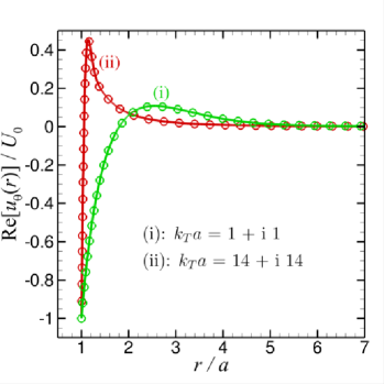
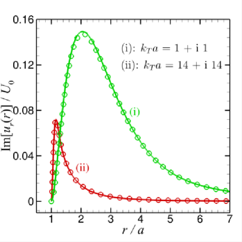
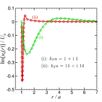
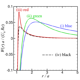
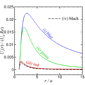
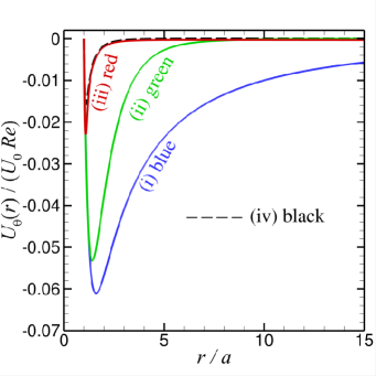
Some representative results will be shown next. In Fig. 1(a-d), we present the real and imaginary parts of the radial and tangential components of the primary velocity from the surface of the sphere at to the far field at . Values of the parameters, and are chosen to reflect the main differences in physical behaviour which are expected to occur if and are larger or smaller compared to unity in different combinations, but subject to the constraint that . The primary flow velocity components are scaled as and ,
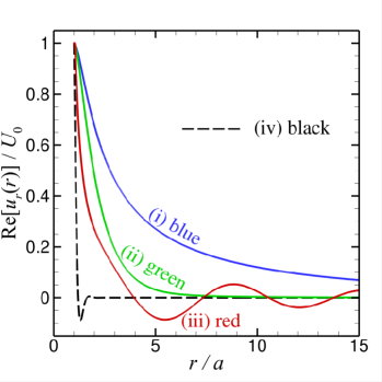
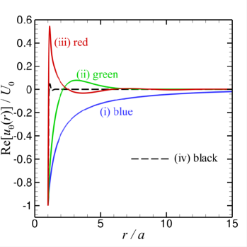
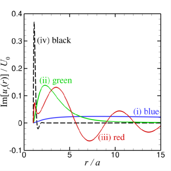
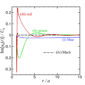
Results for the primary velocity field in Fig. 1(a-d) are given for the following 4 cases:
-
(i)
both , with and (blue curves). The real parts of and have large magnitudes and long range, varying monotonically with . The imaginary parts are also monotonic with but the magnitudes are much smaller than the real parts.
-
(ii)
and with and (green curves). The real and imaginary parts of and have comparable magnitude but only the real part of is monotonic.
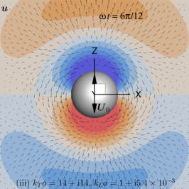
-
(iii)
and the real part of but the imaginary part of is small with and (red curves). The real and imaginary part of and all change sign as increases from the sphere surface.
-
(iv)
both , and has a large imaginary part with and (black curves). In this case, viscous effects dominate and all flow is confined to within a thin boundary layer adjacent to the sphere surface.
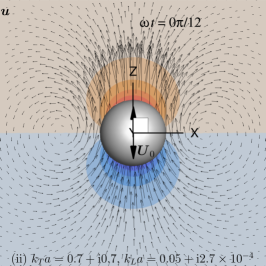
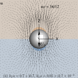
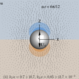
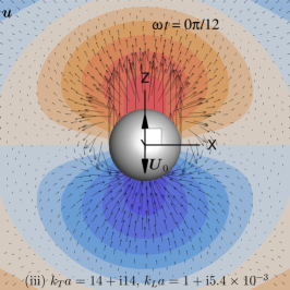
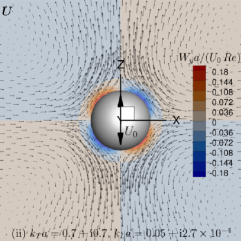
Plots of the primary velocity, , (Eq. 13) and pressure, , (Eq. 8), fields at selected time instants are shown in Fig. 2 for Case (ii) and in Fig. 3 for Case (iii). These images correspond to snapshots of the animation movie that can be found in the supplementary material. Of special interest are the ‘vortex-alike’ structures appearing to the left and right of Fig. 2(a) and (b) in the primary flow patterns.

V Recovery of classical solutions for the primary flow
In this section we will investigate several limits for the primary flow field, namely the small viscosity limit which will lead to potential flow, the large radius limit leading to the flat plate solution and the infinite sound speed that together with large viscosity leads to the classical Stokes flow solution.
V.1 Small viscosity limit, thin boundary layer: potential flow
If viscous effects are small, we expect a very thin boundary layer. From (6), a vanishing viscosity corresponds to the limit and hence for due to the imaginary part of . From (15) we find
and (13) becomes:
| (18) |
This solution is consistent with Landau and Lifshitz [31, p. 286, §74 Problem 1].
If in addition, , we recover the potential flow solution for the fluid velocity around a sphere moving at a constant velocity:
| (19) |
This solution is consistent with Landau and Lifshitz [31, p. 21–22, §10 Problem 2].
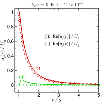
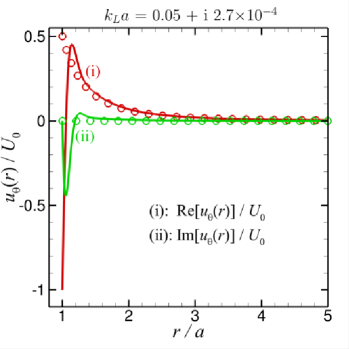
Fig. 4 shows the flow patterns with a carefully selected set of and values, and since it is close to the thin boundary layer limit as and . As demonstrated in Fig. 4, when , outside the thin boundary layer, the results obtained with (13) for the primary velocity field are in good agreement with the results using (18) for the thin boundary layer potential flow limit. Also, for this particular case, as the imaginary part of is close to zero, the imaginary parts of the primary flow velocity components calculated by (18) almost vanish, as displayed by the green circles in Fig. 4. Note that closely follows the potential flow results for , but, in order to satisfy the no-slip condition, bends over sharply in the region to to satisfy the no slip condition . In contrast, the potential flow solution is .
V.2 Large radius: flat plate limit
If the radius of the sphere, , is very large, there are two locations of special interest: the front of the sphere at and the side of the sphere at .
Consider first the side at which and . From (7) we then find since . And setting in (13), we find
| (20) |
For a large sphere, , so and and the velocity becomes:
| (21) |
In the time domain, this is equivalent to the well-known Stokes oscillatory boundary thickness equation [32, 28, 33]: , with , the real part of , and being the distance from the flat surface. Thus, the solution at the side of the sphere tends towards the Stokes vibrating boundary layer theory for a flat plate when the radius of the sphere is large enough.
For the solution in front of the sphere at , in the large or flat plate limit with , the velocity in (7) becomes and with , we have:
| (22) |
Again with for a large sphere, , we have the limiting solution
| (23) |
which represents a plane sound wave propagating out of an oscillating plate.
V.3 Infinite sound speed: (oscillatory) incompressible Stokes flow limit
The incompressibility of the fluid implies that . In this case, we can take the limit of while keeping finite. As such, with the help of the Maclaurin series expansion of , we have
| (24a) | ||||
| (24b) | ||||
Introducing (24) into (13) we have
| (25a) | ||||
| (25b) | ||||
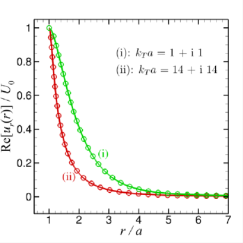
This solution is identical to the solution given by Landau and Lifshitz [31, p. 89, §24 Problem 5], where the velocity was written as , then and . They showed that . This corresponds to our solution with and . It is also consistent with the solution of Eq. (9) from [14]. As shown in Fig. 5, the results obtained by (13) for the primary velocity fields at when (i) and (ii) are in good agreement with the results using (25) for the incompressible Stokes flow limit.
In order to get back the Stokes limit, we have to take the limit as well. By using the Maclaurin series expansions of and , we have
| (26a) | ||||
| (26b) | ||||
| (26c) | ||||
Then the velocity components become:
| (27a) | ||||
| (27b) | ||||
which is the velocity field for a sphere moving in Stokes flow Landau and Lifshitz [31, p. 50–60, §20]. Note that in the above results, terms with cancel each other exactly out.
VI Conclusion
The analytical solution of the flow field around a rigid sphere executing small amplitude rectilinear motion in an compressible fluid was investigated. Both the primary flow, where second order inertial effects were neglected, and the secondary flow were studied. The mathematical form of the equation that governs the primary velocity field is identical to that for the propagation of elastic waves in solids. This allows us to draw on earlier work [19] to obtain analytic solutions. The primary flow field was shown to adhere to all the classical analytical expressions in the small or large viscosity and/or radius limits and is valid for very thin all the way to very thick boundary layers.
The equation that governs the (secondary) streaming flow is analogous to the problem of the flow phenomenon associated with the electrophoretic mobility of a spherical charged particle [23, 24] that enables the streaming velocity field to be expressed readily in terms of the body force and the vorticity.
To the best knowledge of the authors, this is one of the few analytic results in the theory of acoustic boundary layer flow and can serve as benchmark of numerical solution schemes for more complex problems.
Acknowledgements.
This work is supported in part by a Discovery Project Grant (DP170100376) to DYCC. QS is supported by a Discovery Early Career Researcher Award (DE150100169) and a Centre of Excellence Grant (CE140100003) funded by the Australian Research Council.Data Availability
The data that support the findings of this study are available from the corresponding author upon reasonable request.
Appendix A Derivation of the secondary flow field
In this appendix the theoretical solution for the secondary flow field is derived as outlined in Section III.4.
A.1 Symmetry of the streaming equation
From the symmetry condition of the primary velocity field in (7), it follows from (17) that the body force per unit volume that drives the streaming flow must be of the form
| (28) | ||||
where the superscript ‘∗’ denotes the complex conjugate. Explicit expressions for the functions , and in (28) for are
| (29a) | ||||
| (29b) | ||||
| (29c) | ||||
Using this general form for in (17), the streaming velocity must have the following angular and radial dependency
| (30) | ||||
The condition (see Nyborg [21] and Lee and Wang [18]) ensures that the streaming velocity is determined by the single function in (30). The form for the pressure can be inferred from (17)
| (31) |
Instead of solving for the three functions , and , it is more convenient to work in terms of the vorticity field, to eliminate the pressure, . We hereby follow very closely the theory used for electrophoresis of a moving sphere, in particular that of the PhD thesis of Overbeek [23] and although the theory is not identical, many of the mathematical concepts, such as vector manipulation in spherical coordinates and double integration techniques can still be utilised here. Taking the curl of (17) gives . Since both the body force, and the streaming velocity, are independent of the azimuthal angle and have no azimuthal -component, their curl will only have a non-zero component in the -direction along the unit vector, . This then ensures that also points in the direction. From (28) and (30) they are characterised by two functions, and , that are only functions of the radial distance, from the centre of the sphere:
| (32) |
| (33) |
with that characterises the body force in (32) given by
| (34) |
This completes the framework of the axisymmetric streaming flow around a sphere.
A.2 Formal solution of the streaming equation
The method of solution involves deriving an ordinary differential equation for defined in (33) in terms of defined in (32). Then the velocity function, given by (30) can be expressed in terms of to give the solution for the velocity field.
Expressing in spherical polar coordinates, the curl of (17) becomes
| (35) |
that can be integrated immediately to give the vorticity function, , noting that as ,
| (36) |
The integration constant, from the homogeneous solution can be determined from the boundary conditions at the sphere surface, .
In a similar way, the streaming velocity function, can be found by combining (30) and (33) to give
| (37) |
that can be integrated to give , noting that as ,
| (38) |
If the boundary condition of the general problem is that the fluid velocity is prescribed on the sphere surface, this will be satisfied by the primary flow so that the boundary condition of the streaming velocity is . Using (30), this gives and at . From (38), we obtain
| (39) |
The pressure functions, and of the secondary flow in (31) can be readily obtained: can be found by taking the divergence of (17) to eliminate the velocity and can be obtained from the component of (17) to give
| (40) |
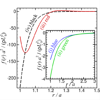
In Fig. 6(a-b), we show results for the function that characterises the curl of the body force that drives the streaming flow, see (32) and the vorticity, of the streaming flow for the set of and values of Cases (i) to (iv) defined in Section IV. Although the body force is derived from the primary velocity field, it has a much shorter range than the primary velocity field. The streaming vorticity, has a much shorter range of at most 3 radii from the sphere surface than the streaming velocity components and given in Fig. 6(c-d). These velocities are scaled as and with the Reynolds number defined as . Thus the time-averaged body force, is significant only within a thin boundary layer from the sphere surface and this is reflected in the observation that the vorticity, is non-zero only within about 5 radii from the surface. However, the streaming velocity field can extend well beyond the range of the streaming vorticity with the typical long ranged characteristics of Stokes flow around a sphere.
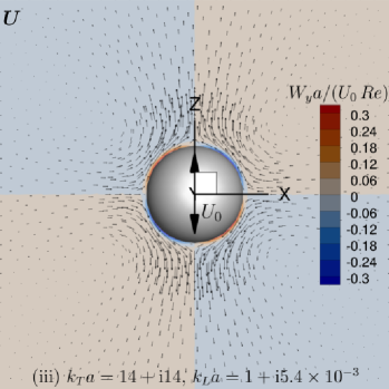
Plots of the secondary velocity, , and vorticity, , are shown in Fig. 7 for Cases (ii) and (iii). The four-lobed velocity profile is clearly visible in Fig. 7 for the secondary streaming flow. Also clearly visible are the eight regions of the secondary streaming flow vorticity in Fig. 7. Even though the vorticity changes sign in each quadrant, the secondary streaming flow velocity does not reverse direction in an individual quadrant. Near the sphere, the axially symmetric steady acoustic streaming flow, due to oscillatory motion of the sphere in the -direction draws fluid towards the sphere in the -plane and re-directs the fluid away from the sphere symmetrically along the directions.
References
- Laurell and Lenshof [2015] T. Laurell and A. Lenshof, Microscale Acoustofluidics (The Royal Society of Chemistry, Cambridge UK, 2015).
- Muller and Bruus [2015] P. Muller and H. Bruus, “Theoretical study of time-dependent, ultrasound-induced acoustic streaming in microchannels,” Phys. Rev. E 92, 063018 (2015).
- Lei, Glynne-Jones, and Hill [2016] J. Lei, P. Glynne-Jones, and M. Hill, “Modal Rayleigh-like streaming in layered acoustofluidic devices,” Physics of Fluids 28, 012004 (2016).
- Doinikov, Thibault, and Marmottant [2018] A. A. Doinikov, P. Thibault, and P. Marmottant, “Acoustic streaming induced by two orthogonal ultrasound standing waves in a microfluidic channel,” Ultrasonics 87, 7–19 (2018).
- Karlsen et al. [2018] J. T. Karlsen, W. Qiu, P. Augustsson, and H. Bruus, “Acoustic streaming and its suppression in inhomogeneous fluids,” Phys. Rev. Lett. 120, 054501 (2018).
- Bach and Bruus [2020] J. S. Bach and H. Bruus, “Suppression of acoustic streaming in shape-optimized channels,” Phys. Rev. Lett. 124, 214501 (2020).
- Subbotin, Kozlov, and Shiryaeva [2019] S. Subbotin, V. Kozlov, and M. Shiryaeva, “Effect of dimensionless frequency on steady flows excited by fluid oscillation in wavy channel,” Physics of Fluids 31, 103604 (2019).
- Pandey, Prabhakaran, and Basu [2019] K. Pandey, D. Prabhakaran, and S. Basu, “Review of transport processes and particle self-assembly in acoustically levitated nanofluid droplets,” Physics of Fluids 31, 112102 (2019).
- Baasch, Doinikov, and Dual [2020] T. Baasch, A. A. Doinikov, and J. Dual, “Acoustic streaming outside and inside a fluid particle undergoing monopole and dipole oscillations,” Physical Review E 101, 013108 (2020).
- Otto, Riegler, and Voth [2008] F. Otto, E. K. Riegler, and G. A. Voth, “Measurements of the steady streaming flow around oscillating spheres using three dimensional particle tracking velocimetry,” Physics of Fluids 20, 093304 (2008).
- Karlsen and Bruus [2015] J. Karlsen and H. Bruus, “Forces acting on a small particle in an acoustical field in a thermoviscous fluid,” Physical Review E 92, 043010 (2015).
- Marshall and Wu [2015] J. S. Marshall and J. Wu, “Acoustic streaming, fluid mixing, and particle transport by a Gaussian ultrasound beam in a cylindrical container,” Physics of Fluids 27, 103601 (2015).
- Lane [1955] C. A. Lane, “Acoustical streaming in the vicinity of a sphere,” The Journal of the Acoustical Society of America 27, 1082–1086 (1955).
- Riley [1966] N. Riley, “On a sphere oscillating in a viscous fluid,” Quart. Journ. Mech. and Applied Math. XIX, 461–472 (1966).
- Davidson and Riley [1971] B. J. Davidson and N. Riley, “Cavitation microstreaming,” Journal of Sound and Vibration 15, 217–233 (1971).
- Longuet-Higgins [1998] M. S. Longuet-Higgins, “Viscous streaming from an oscillating spherical bubble,” Proceedings of the Royal Society of London. Series A: Mathematical, Physical and Engineering Sciences 454, 725–742 (1998).
- Riley [2001] N. Riley, “Steady streaming,” Annu. Rev. Fluid Mech 33, 43–65 (2001).
- Lee and Wang [1990] C. P. Lee and T. G. Wang, “Outer acoustic streaming,” The Journal of the Acoustical Society of America 88, 2367–2375 (1990).
- Klaseboer, Sun, and Chan [2019] E. Klaseboer, Q. Sun, and D. Y. C. Chan, “Helmholtz decomposition and boundary element method applied to dynamic linear elastic problems,” Journal of Elasticity 137, 83–100 (2019).
- Stuart [1966] J. T. Stuart, “Double boundary layers in oscillatory viscous flow,” J. Fluid Mech. 24, 673–687 (1966).
- Nyborg [1953] W. L. Nyborg, “Acoustic streaming due to attenuated plane waves,” The Journal of the Acoustical Society of America 25, 68–75 (1953).
- Strutt (1877) [Lord Rayleigh] J. W. Strutt (Lord Rayleigh), The theory of sound, Volume 1, 1945 reprint (Dover Publications, New York, 1877).
- Overbeek [1941] J. T. G. Overbeek, Theorie der electrophorese, Ph.D. thesis, Utrecht University, H.J. Paris, Amsterdam (1941), English translation http://arxiv.org/abs/1907.05542.
- Jayaraman, Klaseboer, and Chan [2019] A. S. Jayaraman, E. Klaseboer, and D. Y. C. Chan, “The unusual fluid dynamics of particle electrophoresis,” Journal of Colloid and Interface Science 553, 845–863 (2019).
- Eckart [1948] C. Eckart, “Vortices and streams caused by sound waves,” Phys. Rev. 73, 68–76 (1948).
- Gopinath and Trinh [2000] A. Gopinath and E. H. Trinh, “Compressibility effects on steady streaming from a noncompact rigid sphere,” The Journal of the Acoustical Society of America 108, 1514–1520 (2000).
- Hahn, Wang, and Dual [2013] P. Hahn, J. Wang, and J. Dual, “A parallel boundary element algorithm for the computation of the acoustic radiation forces on particles in viscous fluids,” in Proceedings of the 2013 International Conference on Ultrasonics (ICU 2013) May 2-5, 2013 (Singapore, 2013).
- Schlichting [1955] H. Schlichting, Boundary-Layer Theory (McGraw-Hill, 1955).
- Sadhal [2015] S. S. Sadhal, Microscale Acoustofluidics (The Royal Society of Chemistry, 2015) Chap. 12, pp. 256–311.
- Landau and Lifshitz [1970] L. D. Landau and E. M. Lifshitz, Theory of Elasticity, Second (revised) English ed. (Pergamon Press, Great Britain, 1970).
- Landau and Lifshitz [1987] L. D. Landau and E. M. Lifshitz, Fluid Mechanics, Second (revised) English ed. (Pergamon Press, Great Britain, 1987).
- Stokes [2009] G. G. Stokes, “On the effect of the internal friction of fluids on the motion of pendulums,” in Mathematical and Physical Papers (Cambridge University Press, 2009) pp. 1–10.
- Ramos, Cuevas, and Huelsz [2001] E. Ramos, S. Cuevas, and G. Huelsz, “Interaction of Stokes boundary layer flow with a sound wave,” Physics of Fluids 13, 3709–3713 (2001).