Analytical estimation of the signal to noise ratio efficiency in axion dark matter searches using a Savitzky-Golay filter

According to cosmological measurements and the standard model of Big Bang cosmology PLANCK , cold dark matter (CDM) is responsible for about 85% of the total matter in our Universe. CDM does not belong to the Standard Model of particle physics (SM), and as of today the nature of CDM is unknown in spite of the strong evidence of its existence CDM-EVIDENCE . The axion AXION is one of the iconic CDM candidates and originally stems from a breakdown of a new symmetry proposed by Peccei and Quinn PQ , as a very natural solution to the strong $CP$ problem in the SM strongCP . In light of the current galaxy formation dark matter has to be massive, stable, and nonrelativistic, and the axion is predicted to meet all of these conditions. The axion haloscope search proposed by Sikivie utilizes axion-photon coupling and a microwave resonant cavity, which results in the resonant conversion of axions to photons sikivie . This enhances the detected axion signal power drastically. Making the axion haloscope the most promising method for axion dark matter searches in the microwave region. Recent experimental efforts have reached the Dine-Fischler-Srednicki-Zhitnitskii (DFSZ) axion sensitivity ADMX-DFSZ ; 12TB-PRL , where the DFSZ axion can be implemented in grand unified theories (GUT) GUT . If DFSZ cold axion dark matter turns out to constitute 100% of the local dark matter density, that would not only explain the total matter in our Universe, but also support GUT.

Since the resonated axion signal power is only sensitive to the resonant frequency region, and information about axion mass is absent, the most significant and practical figure of merit in axion haloscope searches is the scanning rate scanrate . One of the experimental parameters determining the scanning rate is the signal to noise ratio (SNR) efficiency squared $\epsilon^{2}_{\rm SNR}$ JINST , where the ${\rm SNR}=P^{a\gamma\gamma}_{a}/\sigma_{P_{n}}$ according to the radiometer equation DICKE and we define $\epsilon_{\rm SNR}$ later in equation (2). In the SNR equation, $P^{a\gamma\gamma}_{a}$ is the expected axion signal power for an axion-photon coupling strength sikivie ; scanrate and $\sigma_{P_{n}}$ is the fluctuation in the noise power $P_{n}$. Estimates of the $\epsilon_{\rm SNR}$ have relied on large-statistic simulation data that usually require a lot of computation time and storage resources ADMX ; HAYSTAC ; JHEP . With hints reported in refs. HAYSTAC ; JHEP , in this study we have developed an analytical method to estimate the $\epsilon_{\rm SNR}$ for axion dark matter searches. The $\epsilon_{\rm SNR}$ for axion haloscope searches is frequency-independent or, equivalently, background-independent with the relevant scale factor $\xi$, as demonstrated by refs. HAYSTAC ; JHEP , where $\xi$ is necessary and affected by the combination of power excess bins that are correlated with each other due to background subtraction. In addition, one of our previous works showed that $\epsilon_{\rm SNR}$ is practically the signal power efficiency due to background subtraction JHEP . In another one of our recent works 12TB-PRD , however, we found a subtle effect to the background fluctuation due to background subtraction with a specific condition, which was considered as well.

Inspired by that information, we calculated the signal power efficiency $\epsilon_{P^{a\gamma\gamma}_{a}}=\epsilon_{\rm sig}$ whose effects can first be seen in Fig. 1 and $\xi$ independently using only an arbitrary axion mass and the relevant signal shape information. They showed good agreement with those obtained from large-statistic simulation data. In the end, axion haloscope searches have been observing the coincidence that the frequency independent scale factor $\xi$ is approximately consistent with the $\epsilon_{\rm SNR}$. This was confirmed analytically in this work, if the window length of our background estimator is reasonably wide enough, i.e., at least 5 times the signal window.

The general data analysis procedure for axion haloscope searches studied in this work aims to maximize the significance of an axion signal by weighting and combining data points HAYSTAC . Raw data is acquired through power spectra in the frequency domain. The digitized power spectrum data will have the background noise power stored in frequency bins that are spaced at intervals of the resolution bandwidth (RBW) $\Delta\nu$. The background will feature a baseline characterized by the system noise and its fluctuations. If an axion signal exists amidst the background, it will appear as a lineshape which is distributed to multiple frequency bins. In the case of the standard halo model, the lineshape is a boosted Maxwellian TURNER

This lineshape depends on the axion frequency $\nu_{a}$, $r=v_{E}/v_{\mathrm{rms}}$, and $\expectationvalue{\beta^{2}}=1.5v_{\mathrm{rms}}^{2}/c^{2}$, where $v_{E}$ is the velocity of Earth with respect to the galaxy halos, $v_{\mathrm{rms}}$ is the local circular velocity of the galaxy, and $c$ is the speed of light. In the analysis stage an axion signal window $\Delta\nu_{a}$ is used where the integral of $f(\nu)$ from $\nu_{a}$ to $\nu_{a}+\Delta\nu_{a}$ nears unity. The axion signal power is weak; for instance in the CAPP-12TB experiment it was on the order of tens of yoctowatts 12TB-PRL , making it difficult to distinguish from noise fluctuations. Therefore the data is further processed in a way that increases the SNR of an expected signal.

Following the conventional methods of haloscope data analysis, an axion signal, should it exist, will appear as a sharp peak on the background as shown in Fig. 1. This is also replicable by inserting a software-injected axion signal into an experiment’s background. Then the SNR of an input signal, which will have its background perfectly removed, can be compared with the SNR of signal which has its background removed by a fit. Examples of a fit estimator are a $\chi^{2}$ fit such as in refs. 12TB-PRL ; CAPP-8TB-PRL or a Savitzky-Golay (SG) filter SGFILTER as seen in refs. 12TB-PRD ; HAYSTAC . In this work we will be focusing on the latter as it does not require a functional form of the background structure, can handle zero-fluctuation data like the axion signal power considered in axion dark matter searches, and its estimates are fully predictable.

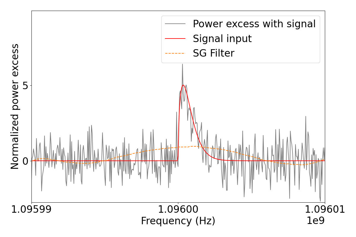
Typically any estimate of the background will be affected by a signal such as the one shown in Fig. 1 and due to this the output SNR will not recover 100% of the input. The difference in the input and output SNR can be expressed through an efficiency term $\epsilon_{\rm SNR}$

where we define $\epsilon_{\rm sig}=\delta_{\rm output}/\delta_{\rm input}$ for input and output signal powers $\delta_{\rm input}$ and $\delta_{\rm output}$. $\epsilon_{\rm sig}$ is approximately equal to $\mathrm{SNR}_{\mathrm{output}}/\mathrm{SNR}_{\mathrm{input}}$ as $\sigma_{P_{n}}$ for input and output are practically equal JHEP . The frequency-independent scale factor $\xi$ is used to offset the bin-to-bin correlations that are introduced from background subtraction HAYSTAC ; JHEP . This value is set to the width of the Gaussian fit for the normalized power excess of the output. In terms of input, the normalized power excess’ Gaussian width should be equal to one.

We will first proceed to discuss how to obtain the value of $\epsilon_{\rm sig}$. Using an SG filter as a background estimate, it is possible to construct a signal following equation (1) on a flat background that does not include any noise fluctuations. The input signal in units of arbitrary power excess will be distributed into $n_{c}=\Delta\nu_{a}/\Delta\nu$ frequency bins that have a resolution bandwidth $\Delta\nu$, assuming that the first bin’s frequency is equal to $\nu_{a}$. The input signal power in the $k$th bin is

where $\delta_{a}$ is a multiplicative constant that represents $P_{a}^{a\gamma\gamma}$ and $L_{k}$ are the fractions of axion signal power stored into the $k$th bin. While our SG filter is designed to describe the background only, it will be applied to the set of $\delta_{k}$ (the red line in the left panel of Fig. 2) to parametrize the spectrum containing the signal as well as the flat background. As also seen in the left panel of Fig. 2, the smoothing from the filter, shown as orange dashed lines, does not fit the background properly around the signal region when one is present. The exact response of the SG filter is

with $\sum_{k}c_{k}=1$. $\hat{\delta}_{k}$ is the SG filter’s estimate of the background for the cases considered in this work. What is considered to be the signal power after background subtraction will be $\delta^{\prime}_{k}=\delta_{k}-\hat{\delta}_{k}$ (the blue line in the left panel of Fig. 2). The coefficients $c_{k}$ only depend on the SG filter parameters, window length $2W+1$ and polynomial order $d$. As $\sum_{k}c_{k}=1$, an estimation done with the SG filter acts like a weighted average. The same $2W+1$ values are applied to the coefficients when obtaining each separate $\hat{\delta}_{k}$ with different $k$. A few examples of SG filter coefficients depending on the parameters can be seen in the right panel of Fig. 2. The coefficients can be obtained from its definition in the original paper SGFILTER , and it can be fit using a $d$th-order polynomial (for even $d$). It is also easy to obtain $c_{k}$ in SG filter packages in programming languages PYTHON .

$\delta_{k}$ and $\delta_{k}^{\prime}$ are combined according to the analysis procedure HAYSTAC . Following this all further combination processes use inverse-variance weighting. For any stage of combination, this means that a combined power $\delta^{\mathrm{combined}}$ and its error $\sigma^{\mathrm{combined}}$ will follow

for all relevant powers $\delta_{k}^{\mathrm{before}}$ and their errors $\sigma_{k}^{\mathrm{before}}$ used for the combination. In the presence of $\sigma_{k}^{\mathrm{before}}$, the weights $w_{k}=(\sigma_{k}^{\mathrm{before}})^{-2}$, except during the coadding process to obtain the grand spectrum. In this case $w_{k}=(\sigma_{k}^{\mathrm{before}})^{-2}L_{k}$.

Now we will obtain the SNR ratio through the axion signal power ratio: $\epsilon_{\rm sig}=\delta_{\rm output}/\delta_{\rm input}$. As the SG filter response of each $\delta_{k}$ is up to the multiplicative constant $\delta_{a}$, its effects cancel out in the value of $\epsilon_{\rm sig}$. Therefore the value of $\epsilon_{\rm sig}$ will not change when signal power is added in a way that changes $\delta_{a}$ by the same ratio for both input and output, such as vertical combination. This was confirmed to be in agreement with large-statistic simulations which do include vertical combination and will be further discussed in Sec. 4. Rebinning, or equivalently RBW reduction, however, does affect the results and will be discussed in Sec. 3. If this process is not used, the only leftover contribution to the analysis process is coadding bins. We can now use equation (5) with $\delta_{k}^{\rm before}=\delta_{k}$ or $\delta^{\prime}_{k}$ and $w_{k}=L_{k}$. For the particular bin that coincides with the axion frequency, the signal power after coadding $n_{c}$ bins is

and

resulting in

where if $\absolutevalue{i-j}>W$, $c_{i-j}=0$. As $\epsilon_{\rm sig}$ does not take any noise fluctuations into account it does not carry any error. Hence, this can be used as an exact value instead of an estimate. The value of $\epsilon_{\rm sig}$ depending on $W$ is shown in the right panel of Fig. 3.

The remaining factor in $\epsilon_{\rm SNR}$, $\xi$, will be obtained next. For this calculation there will be no axion signal, and only the background is considered. This time the inputs will be multiple independent random variables $x_{k}$ that follow a Gaussian distribution $\mathcal{N}\left(\bar{x}_{k},\sigma_{x_{k}}^{2}\right)$. The normalized power is

making $\sigma_{X_{k}}$ one. The estimated background using the SG filter for $X_{k}$ is

The power excess is $X^{\prime}_{k}=X_{k}-\hat{X}_{k}$. Ideally the estimate $\hat{X}_{k}$ is equal to $\bar{X}_{k}=\bar{x}_{k}/\sigma_{x_{k}}$ as $X_{k}$ follows an $\mathcal{N}\left(\bar{X}_{k},\sigma_{X_{k}}^{2}\right)$ distribution. It was observed 12TB-PRD and is known that the standard deviation of $X^{\prime}_{k}$ depends on $W$ and is reduced by

where $b=9/8$ for $d=2$ and $b=225/128$ for $d=4$ if $W$ is large enough SGFILTER-PROPERTIES . Therefore $X^{\prime}_{k}$ must be further divided by $\xi_{\rm SG}$ to make it follow an $\mathcal{N}\left(0,\sigma_{X^{\prime}_{k}}^{2}\right)$ distribution with $\sigma_{X^{\prime}_{k}}=1$. The normalized power excess for SG filter estimated data is

The use of normalized power excess to obtain $\xi$ is valid as it is independent of the background HAYSTAC ; JHEP and so are the coefficients $c_{k}$. The exception to this would be when background subtraction is done poorly or is biased, which will be explored in Sec. 4. Here we will continue with the assumption that $\hat{X}_{k}$ is an unbiased estimate of $\bar{X}_{k}$. Similar to the discussion from before, a vertical combination combines different raw spectra, so the random variables that are combined must be independent, and therefore it does not affect the distribution of $X_{k}$ nor $X^{\prime}_{k}$.

Now equation (5) is used again with $\delta_{k}^{\rm before}=X_{k}$ or $X^{\prime}_{k}$ and $w_{k}=L_{k}$ with $\sigma_{k}^{\rm before}=\sigma_{X_{k}}$ or $\sigma_{X^{\prime}_{k}}$. The normalized input noise at the axion frequency corresponding to $k=0$ after coadding is

which has a standard deviation of one as expected from $n_{c}$ independent random variables. Coadding the set of $X^{\prime}_{k}$ we have

$X^{\prime}_{k}$ are no longer independent to each other since each can include overlapping terms that can range from $X_{-W}$ to $X_{W+n_{c}-1}$ according to equation (12). Therefore this equation is used to decouple $X_{\rm coadded}^{\prime}$ into independent random variables $X_{i}$. The coefficient value in front of $X_{i}$ is

with the constraints $L_{i}=0$ for $i<0$ or $i\geq n_{c}$, $c_{k}=0$ for $k<-W$ or $k>W$. The standard deviation of $X_{\rm coadded}^{\prime}$, which corresponds to the frequency independent scale factor $\xi$, is

The value of $\xi$ for an SG filter with varying $W$ can be seen in Fig. 4.

It can be observed that both $\epsilon_{\rm sig}$ and $\xi$ become closer to unity as $W$ increases. This can be understood intuitively since the SG filter is an estimate for a background in the context of this raw spectrum. As $W$ becomes larger, the SG filter will tend to “ignore” the signal and therefore retain more of its power, without being too biased. On the other hand, for noise fluctuations when more points are taken into consideration, the bin-to-bin correlations are smaller as $W$ increases since the sum of all $c_{k}$ is one, meaning that the contribution of each bin is smaller, as seen from the right panel of Fig. 2. This also tends to average out to $\bar{X}_{k}$.

By merging $n_{m}$ bins and increasing the RBW value to $\Delta\nu^{\rm merged}=n_{m}\Delta\nu$, the power spectrum undergoes a process called rebinning. This process combines the $n_{m}$ bins according to equation (5). For the calculation of $\epsilon_{\rm sig}$, the signal powers after rebinning with $w_{k}=1$ and $\delta^{\rm before}_{k}=\delta_{k}$ are

which are the averages of the signal powers over $n_{m}$ bins.

A coadded bin after rebinning will coadd $n_{c}/n_{m}$ bins, with the weights used for coadding $w_{k}=L_{k}^{\rm merged}$ following

Obtaining $\epsilon_{\rm sig}$ is straightforward in the sense that the rebinning is applied to each $\delta_{k}$, then the rebinned bins are coadded.

and $\epsilon^{\rm merged}_{\rm sig}=\delta^{\rm merged}_{\rm output}/\delta^{\rm merged}_{\rm input}$. For both signal input and output the resulting SNR values have been shown to decrease, as seen in ref. 12TB-PRL . While this is a drawback of rebinning, the number of rescan candidates is also reduced, which is an advantage that could be considered as a tradeoff 12TB-PRL ; 12TB-PRD .

Now the rebinned counterpart for noise, $X_{k}^{\rm merged}$ and $X_{k}^{\prime\mathrm{merged}}$, will yield a modified $\xi^{\rm merged}$. Using equation (16) and the fact $X_{k}$ and $X_{k}^{\prime}$ are combined in a linear fashion, the only part of the equation that needs modification is $L_{k}$, which must be expressed in terms of $L_{k}^{\rm merged}$. For any $n_{m}$ bins merged, $X_{k}^{\rm merged}$ and $\sigma_{X_{k}^{\rm merged}}$ are as follows

where the total number of $i$ is $n_{m}$. The same applies for $X_{k}^{\prime\rm merged}$. All $n_{m}$ merged bins will now be coadded with the same $L_{k}^{\rm merged}$ value instead of the $n_{m}$ different $L_{k}$ values (e.g., $L_{0}$, $L_{1}$, $\cdots$, $L_{n_{m}-1}$) from before. The coadded and normalized values are

where the floor function $\lfloor{x}\rfloor$ returns the largest integer smaller or equal to $x$. $\mathcal{X}_{\rm coadded}$ has a standard deviation of one as expected. For $\mathcal{X}^{\prime}_{\rm coadded}$, the standard deviation, or equivalently, the frequency independent scale factor after rebinning $\xi^{\rm merged}$ is obtained as

and the relevant results are shown in table 1. $C_{i}^{\rm merged}$ is also different from $C_{i}$ since it also includes $L^{\rm merged}_{k}$ as

As shown in equation (21), the rebinned set of $X^{\prime\rm merged}_{k}$ in equation (21) is separable into $X^{\prime}_{k}$ using equation (20) and ultimately $X_{k}$ via equation (12). By unpacking the merged variables fully into independent random variables, the calculation of $\xi^{\rm merged}$ in equation (22) becomes as straightforward as $\xi$ in equation (16).

Putting the effects of rebinning from both sides together, the SNR efficiency $\epsilon_{\rm SNR}^{\rm merged}=\epsilon^{\rm merged}_{\rm sig}/\xi^{\rm merged}$ is smaller than $\epsilon_{\rm SNR}$, which is a separate effect from the aforementioned SNR decrease reported in ref. 12TB-PRL . This is later shown in table 1 ($\epsilon_{\rm SNR}$ and $\epsilon_{\rm SNR}^{\rm merged}$) and Fig. 6 (blue and orange lines), although the difference is smaller for large $W$. While $\epsilon^{\rm merged}_{\rm sig}<\epsilon_{\rm sig}$ and $\xi^{\rm merged}<\xi$, the difference between $\epsilon_{\rm sig}$ and its rebinned counterpart is larger than the change in $\xi$, leading to a decrease in SNR efficiency after rebinning.

So far the value of $\epsilon_{\rm SNR}$ has been obtained given $\nu_{a}$, $\Delta\nu_{a}$, and $\Delta\nu$. In order to see if this agrees with previously used large-statistic simulations, an axion signal was inserted by software using realistic CAPP-12TB background data. The input CAPP-12TB background shapes use the function and its parameters that were obtained from the $\chi^{2}$ fit in the original data analysis 12TB-PRL . Another background was constructed for comparison as well, which used the same parameters except for one that described the cavity bandwidth, which was multiplied by 20. This ensured that the structure of the cavity was not seen in this background, and instead was a “smooth” one. Both backgrounds are compared in Fig. 5. Each simulation was done 10000 times with pseudo-random-generated noise to obtain a sufficient amount of statistics, with an axion signal injected near 1.096 GHz. We will denote the results for the two types of backgrounds as “12TB” and “smooth,” respectively, e.g., $\epsilon_{\rm SNR}^{\rm 12TB}$ or $\xi^{\rm smooth}$. Since the simulations follow the CAPP-12TB analysis parameters, there is rebinning. Hence the relevant values should be compared with $\epsilon_{\rm SNR}^{\rm merged}$ and $\xi^{\rm merged}$.

Compared to the time and disk space needed for large-statistic simulations, obtaining the values analytically for the same parameters is practically interactive, taking less than a minute while using only computer memory. The results can be compared in table 1 and Fig. 6.

As seen from the simulation results, a smooth background matches the rebinned analytical calculations well, but the 12TB background does not. This is expected from ref. SGFILTER-PROPERTIES , i.e., as $W$ increases the background estimation begins to show bias for the 12TB background shown in Fig. 5, similar to the SG filter’s tendency to “ignore” the axion signal, as mentioned earlier. Looking at $\xi^{\rm 12TB}$, $\xi^{\rm smooth}$, and $\xi^{\rm merged}$ in table 1, this bias propagates to the grand spectrum and becomes evident from $2W+1=801$. Furthermore, the bias even shows a positive correlation when $2W+1=1001$, which has also been noted in HAYSTAC . In terms of $\epsilon_{\rm SNR}$ in Fig. 6, which combines the effects of $\epsilon_{\rm sig}$ and $\xi$, we can see the bias become evident from $2W+1=601$.

The bias shown in the normalized power excess in the CAPP-12TB background suggests that there is a limit to using larger $W$ for SG filters and this can affect both $\epsilon_{\rm SNR}$ and $\xi$ in an undesirable manner. Using the analytical calculations can work as a time-efficient way to obtain the SNR efficiency and a predictor for $\xi$ during data analysis. If the resulting $\xi$ from data analysis is noticeably different compared to its predicted value, this could indicate that there is bias in background subtraction. As seen in Fig. 7, there is a pattern in the bias that comes from the cavity response in the CAPP-12TB background. The bias is not always obvious as even the $2W+1=401$ estimate shows a slight bump near the center of the normalized power excess, but only after one hundred different power spectra have been averaged. While this ultimately did not dramatically affect the results in table 1, there is a certain upper limit in $W$ which could be used before it becomes inaccurate. This, however, does not suggest a limitation of this analytical method but rather acts as a confidence check for background subtraction to look out for instances such as the one shown in Fig. 7. The verification of proper background subtraction is necessary in the analysis procedure not only for the correct estimation of SNR but also for obtaining unbiased power excesses.

In table 2, as further validation, two other experiments that used the SG filter for background subtraction and provided the required parameters ($\nu_{a}$, $\Delta\nu$, $W$, $d$, $n_{m}$) have their $\xi$ and $\epsilon_{\rm SNR}$ values compared with the analytical method.

We report a fully analytical estimation of the signal to noise ratio efficiency $\epsilon_{\rm SNR}$ in axion dark matter searches employing an SG filter for a background estimate. Provided the background estimation is properly done with appropriate SG filter parameters like the blue colored data shown in Fig. 7, this approach provides us with the $\epsilon_{\rm SNR}$ interactively, using only an arbitrary axion mass and the relevant shape information, without relying on large-statistic simulation data, reflecting the background information and the expected axion signal power obtained from a real experiment. By comparing our $\xi$ or $\xi^{\rm merged}$ with the width of the normalized grand power spectrum from the experimental data, one can also quickly cross check the reasonableness of the error estimation as well as contamination of non-Gaussian components in the experimental data. Axion haloscope searches have been observing the coincidence that the frequency independent scale factor $\xi$ is approximately consistent with $\epsilon_{\rm SNR}$. This was confirmed analytically in this work, when the window length of the SG filter is reasonably wide enough, i.e., at least 5 times the signal window.