Analytical bounds on the local Lipschitz constants of affine-ReLU functions

The huge successes of deep neural networks have been accompanied by the unfavorable property of high sensitivity. As a result, for many networks a small perturbation of the input can produce a huge change in the output [13]. These sensitivity properties are still not completely theoretically understood, and raise significant concerns when applying neural networks to safety-critical and other applications. This establishes a strong motivation to obtain a better theoretical understanding sensitivity.

One of the main tools in analyzing the sensitivity of neural networks is the Lipschitz constant, which is a measure of how much the output of a function can change with respect to changes in the input. Analytically computing the exact Lipschitz constant of neural networks has so far been unattainable due to the complexity and high-dimensionality of most networks. As feedforward neural networks consist of a composition of functions, a conservative upper bound on the Lipschitz constant can be determined by calculating the product of each individual function’s Lipschitz constant [13]. Unfortunately, this method usually results in a very conservative bound.

Calculating or estimating tighter bounds on Lipschitz constants has recently been approached using optimization-based methods [11, 8, 3, 17, 6]. The downside to these approaches is that they usually can only be applied to small networks, and also often have to be relaxed, which invalidates any guarantee on the bound.

In summary, the current state of Lipschitz analysis of neural networks is that the function-by-function approach yields bounds which are too loose, and holistic approaches are too expensive for larger networks. In this paper, we explore a middle ground between these two approaches by analyzing the composite of two functions, the affine-ReLU function, which represents a common layer used in modern neural networks. This function is simple enough to obtain analytical results, but complex enough to provide tighter bounds than the function-by-function analysis. We can also combine the constants between layers to compute a Lipschitz constant for the entire network. Furthermore, our analytical approach leads us to develop intuition behind the structure of neural network layers, and shows how the different components of the layer (e.g. the linear operator, bias, nominal input, and size of the perturbation) contribute to sensitivity.

The high sensitivity of deep neural networks has been noted as early as [13]. This work conceived the idea of adversarial examples, which have since become a popular area of research [4]. One tool that has been used to study the sensitivity of networks is the input-output Jacobian [9, 12], which gives a local estimate of sensitivity but generally provides no guarantees.

Lipschitz constants are also a common tool to study sensitivity. Recently, several studies have explored using optimization-based approaches to compute the Lipschitz constant of neural networks. The work of [11] presents two algorithms, AutoLip and SeqLip, to compute the Lipschitz constant. AutoLip reduces to the standard conservative approach, while SeqLip is an optimization which requires a greedy approximation for larger networks. The work of [8] presents a sparse polynomial optimization (LiPopt) method which relies on the network being sparse. To apply this technique to larger networks, the authors have to first prune the network to increase sparsity. A semidefinite programming technique (LipSDP) is used in [3], but in order to apply the results to larger networks, a relaxation must be used which invalidates the guarantee. Another approach is that of [17], in which linear programming is used to estimate Lipschitz constants. Finally, [6] proposes exactly computing the Lipschitz constant using mixed integer programming, which is very expensive and can only be applied to very small networks.

Other work has considered computing Lipschitz constants in the context of adversarial examples [10, 15, 16]. While these works use Lipschitz constants and similar mathematical analysis, their focus is on classification, and it is not clear how or if these techniques can be adapted to provide guaranteed upper Lipschitz bounds for larger networks. Additionally, other work has considered constraining the Lipschitz constant as a means to regularize a network [5, 14, 1]. Finally, we note that in this work we study affine-ReLU functions which are commonly used in neural networks, but we are not aware of any work that has directly analyzed these functions except for [2].

Our main contributions are that develop analytical upper bounds on the local Lipschitz constant of affine-ReLU function. We show how these bounds can be combined to create a bound on an entire feedforward network, and also how we can compute our bounds even for large layers.

In this paper, we use non-bold lowercase and capital ($a$ and $A$) to denote scalars, bold lowercase ($\boldsymbol{\mathbf{a}}$) to denote vectors, and bold uppercase ($\boldsymbol{\mathbf{A}}$) to denote matrices. Similarly, we use non-bold to denote scalar-valued functions ($f(\cdot)$) and bold to denote vector-valued functions ($\boldsymbol{\mathbf{f}}(\cdot)$). We will use inequalities to compare vectors, and say that $\boldsymbol{\mathbf{a}}>\boldsymbol{\mathbf{b}}$ holds if all corresponding pairs of elements satisfy the inequality. Additionally, unless otherwise specified, we let $\lVert\cdot\rVert$ denote the 2-norm.

Affine functions are ubiquitous in deep neural networks, as convolutional, fully-connected, and normalization functions are all affine. An affine function can be written as $\boldsymbol{\mathbf{f}}(\boldsymbol{\mathbf{x}})=\boldsymbol{\mathbf{A}}\boldsymbol{\mathbf{x}}+\boldsymbol{\mathbf{b}}$ where $\boldsymbol{\mathbf{A}}\in\mathbb{R}^{m\times n}$, $\boldsymbol{\mathbf{x}}\in\mathbb{R}^{n}$, and $\boldsymbol{\mathbf{b}}\in\mathbb{R}^{m}$. Note that since we are considering neural networks, without loss of generality we can define $\boldsymbol{\mathbf{x}}$ to be a tensor that has been reshaped into a 1D vector. We note that we can redefine the origin of the domain of an affine function to correspond to any point $\boldsymbol{\mathbf{x}}_{0}$. More specifically, if we consider the system $\boldsymbol{\mathbf{A}}\boldsymbol{\mathbf{x}}{+}\boldsymbol{\mathbf{b}}_{0}$ and nominal input $\boldsymbol{\mathbf{x}}_{0}$, we can redefine $\boldsymbol{\mathbf{x}}$ as $\boldsymbol{\mathbf{x}}_{0}{+}\boldsymbol{\mathbf{x}}$ in which case the affine function becomes $\boldsymbol{\mathbf{A}}\boldsymbol{\mathbf{x}}{+}\boldsymbol{\mathbf{A}}\boldsymbol{\mathbf{x}}_{0}{+}\boldsymbol{\mathbf{b}}_{0}$. We then redefine the bias as $\boldsymbol{\mathbf{b}}\coloneqq\boldsymbol{\mathbf{b}}_{0}{+}\boldsymbol{\mathbf{A}}\boldsymbol{\mathbf{x}}_{0}$, which gives us the affine function $\boldsymbol{\mathbf{A}}\boldsymbol{\mathbf{x}}{+}\boldsymbol{\mathbf{b}}$. In this paper, we will use the form $\boldsymbol{\mathbf{A}}\boldsymbol{\mathbf{x}}{+}\boldsymbol{\mathbf{b}}$ to represent an affine function that has been shifted so that the origin is at $\boldsymbol{\mathbf{x}}_{0}$, and $\boldsymbol{\mathbf{x}}$ represents a perturbation from $\boldsymbol{\mathbf{x}}_{0}$.

The rectified linear unit (ReLU) is widely used as an activation function in deep neural networks. The ReLU is simply the elementwise maximum of an input and zero: $\boldsymbol{\mathbf{relu}}(\boldsymbol{\mathbf{y}})=\max(\boldsymbol{\mathbf{0}},\boldsymbol{\mathbf{y}})$. The ReLU is piecewise linear, and can therefore be represented by a piecewise linear matrix. To define this matrix, we will first define the following function which indicates if a value is non-negative: $\text{ind}(y)=\{1~{}\text{if}~{}y<0,~{}~{}0~{}\text{if}~{}y\leq 0\}$. We will define the elementwise version of this function as $\boldsymbol{\mathbf{ind}}:\mathbb{R}^{m}\rightarrow\{0,1\}^{m}$. By defining $\boldsymbol{\mathbf{diag}}:\mathbb{R}^{m}\rightarrow\mathbb{R}^{m\times m}$ as the function which creates a diagonal matrix from a vector, we define the ReLU matrix $\boldsymbol{\mathbf{R}}_{\boldsymbol{\mathbf{y}}}$ and ReLU function $\boldsymbol{\mathbf{relu}}$ as follows

$$\boldsymbol{\mathbf{R}}_{\boldsymbol{\mathbf{y}}}=\boldsymbol{\mathbf{diag}}(\boldsymbol{\mathbf{ind}}(\boldsymbol{\mathbf{y}})),~{}~{}~{}~{}~{}~{}~{}~{}~{}~{}~{}~{}~{}~{}\boldsymbol{\mathbf{relu}}(\boldsymbol{\mathbf{y}})=\boldsymbol{\mathbf{R}}_{\boldsymbol{\mathbf{y}}}\boldsymbol{\mathbf{y}}.$$

(1)

Note that $\boldsymbol{\mathbf{R}}_{\boldsymbol{\mathbf{y}}}$ is a function of $\boldsymbol{\mathbf{y}}$, but to make our notation clear we choose to denote the dependence on $\boldsymbol{\mathbf{y}}$ using a subscript rather than parentheses.

Note that ReLUs are naturally related to the geometric concept of orthants, which are a higher dimensional generalization of quadrants in $\mathbb{R}^{2}$ and octants in $\mathbb{R}^{3}$. The $m$-dimensional space $\mathbb{R}^{m}$ has $2^{m}$ orthants. Furthermore, the matrix $\boldsymbol{\mathbf{R}}$ can be interpreted as an orthogonal projection matrix, which projects $\boldsymbol{\mathbf{y}}$ onto a lower-dimensional space of $\mathbb{R}^{m}$. In $\mathbb{R}^{3}$ for example, $\boldsymbol{\mathbf{R}}$ will represent a projection onto either the origin (when $\boldsymbol{\mathbf{R}}=\boldsymbol{\mathbf{0}}$), a coordinate axis, a coordinate plane, or all of $\mathbb{R}^{3}$ (when $\boldsymbol{\mathbf{R}}=\boldsymbol{\mathbf{I}}$). Each orthant in $\mathbb{R}^{m}$ corresponds to a linear region of the ReLU function, so since there are $2^{m}$ orthants there are $2^{m}$ linear regions.

We define an affine-ReLU function as a ReLU composed with an affine function. In a neural network, these represent one layer, e.g. a convolution or fully-connected function with a ReLU activation. Using the notation in (1), we can write an affine-ReLU function as

$$\boldsymbol{\mathbf{relu}}(\boldsymbol{\mathbf{A}}\boldsymbol{\mathbf{x}}+\boldsymbol{\mathbf{b}})=\boldsymbol{\mathbf{R}}_{\boldsymbol{\mathbf{A}}\boldsymbol{\mathbf{x}}+\boldsymbol{\mathbf{b}}}(\boldsymbol{\mathbf{A}}\boldsymbol{\mathbf{x}}+\boldsymbol{\mathbf{b}}).$$

(2)

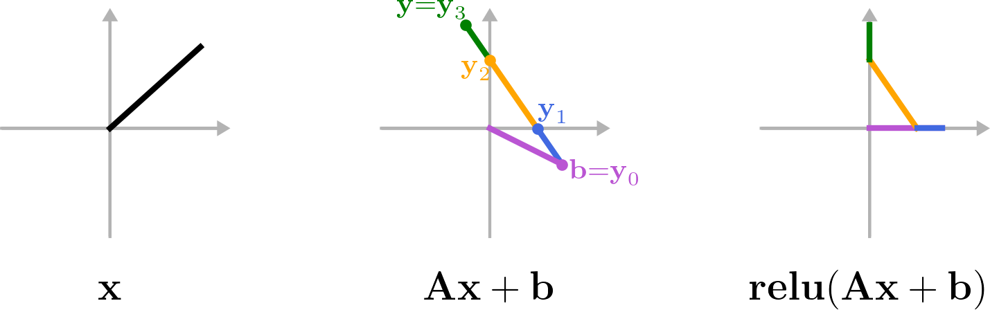
Using Fig. 2 as a reference, we note that the vector $\boldsymbol{\mathbf{y}}=\boldsymbol{\mathbf{A}}\boldsymbol{\mathbf{x}}+\boldsymbol{\mathbf{b}}$ will lie in several different orthants of $\mathbb{R}^{m}$, which are the linear regions of the ReLU function. As a result, $\boldsymbol{\mathbf{relu}}(\boldsymbol{\mathbf{A}}\boldsymbol{\mathbf{x}}+\boldsymbol{\mathbf{b}})$ can be represented as a sum across the linear regions (i.e. orthants) of the function. For each $\boldsymbol{\mathbf{x}}$, there will be some number $p$ of linear regions, and we define the points at which $\boldsymbol{\mathbf{y}}$ transitions between linear regions as $\boldsymbol{\mathbf{y}}_{i}=\alpha_{i}\boldsymbol{\mathbf{A}}\boldsymbol{\mathbf{x}}+\boldsymbol{\mathbf{b}}$ for $i=1,...,p-1$ and where $0<\alpha_{i}<1$ and $\alpha_{i}>\alpha_{i-1}$. We also define $\alpha_{0}=0$ and $\alpha_{p}=1$ so that $\boldsymbol{\mathbf{y}}_{0}=\boldsymbol{\mathbf{b}}$ and $\boldsymbol{\mathbf{y}}_{p}=\boldsymbol{\mathbf{y}}$. The transition vectors $\boldsymbol{\mathbf{y}}_{i}$ can be determined for a given $\boldsymbol{\mathbf{x}}$ by determining the value of $\alpha_{i}$ for which elements of $\boldsymbol{\mathbf{y}}_{i}=\alpha_{i}\boldsymbol{\mathbf{A}}\boldsymbol{\mathbf{x}}+\boldsymbol{\mathbf{b}}$ equal zero. With these vectors defined, we note that any vectors $\boldsymbol{\mathbf{y}}_{i-1}$ and $\boldsymbol{\mathbf{y}}_{i}$ will lie in or at the boundary of the same orthant, and we define $\boldsymbol{\mathbf{R}}_{i}$ as the ReLU matrix corresponding to that orthant. Therefore, we can write the net change of the affine-ReLU function across the orthant adjacent to $\boldsymbol{\mathbf{y}}_{i-1}$ and $\boldsymbol{\mathbf{y}}_{i}$ as

$\displaystyle\boldsymbol{\mathbf{R}}_{i}(\boldsymbol{\mathbf{y}}_{i}-\boldsymbol{\mathbf{y}}_{i-1})=\boldsymbol{\mathbf{R}}_{i}(\alpha_{i}\boldsymbol{\mathbf{A}}\boldsymbol{\mathbf{x}}+\boldsymbol{\mathbf{b}}-(\alpha_{i-1}\boldsymbol{\mathbf{A}}\boldsymbol{\mathbf{x}}+\boldsymbol{\mathbf{b}}))=(\alpha_{i}-\alpha_{i-1})\boldsymbol{\mathbf{R}}_{i}\boldsymbol{\mathbf{A}}\boldsymbol{\mathbf{x}}.$

(3)

Next, we define $\Delta\alpha_{i}\coloneqq\alpha_{i}-\alpha_{i-1}$ and note that $\sum_{i=1}^{p}\Delta\alpha_{i}=1$. Noting that the change from the $\boldsymbol{\mathbf{0}}$ to $\boldsymbol{\mathbf{b}}$ segment of $\boldsymbol{\mathbf{y}}$ is $\boldsymbol{\mathbf{R}}_{\boldsymbol{\mathbf{b}}}(\boldsymbol{\mathbf{b}}-\boldsymbol{\mathbf{0}})=\boldsymbol{\mathbf{R}}_{\boldsymbol{\mathbf{b}}}\boldsymbol{\mathbf{b}}$ (see Fig. 2), we can write the affine-ReLU function as

$\displaystyle\boldsymbol{\mathbf{relu}}(\boldsymbol{\mathbf{A}}\boldsymbol{\mathbf{x}}+\boldsymbol{\mathbf{b}})$

$\displaystyle=\boldsymbol{\mathbf{R}}_{\boldsymbol{\mathbf{b}}}\boldsymbol{\mathbf{b}}+\sum_{i=1}^{p}\Delta\alpha_{i}\boldsymbol{\mathbf{R}}_{i}\boldsymbol{\mathbf{A}}\boldsymbol{\mathbf{x}}.$

(4)

We will analyze the sensitivity of the affine-ReLU functions using a Lipschitz constant, which measures how much the output of a function can change with respect to changes in the input. The Lipschitz constant of a function $\boldsymbol{\mathbf{f}}:\mathbb{R}^{n}\rightarrow\mathbb{R}^{m}$ is $L=\sup_{\boldsymbol{\mathbf{x}}_{0}\neq\boldsymbol{\mathbf{x}}_{1}}\lVert\boldsymbol{\mathbf{f}}(\boldsymbol{\mathbf{x}}_{1})-\boldsymbol{\mathbf{f}}(\boldsymbol{\mathbf{x}}_{0})\rVert/\lVert\boldsymbol{\mathbf{x}}_{1}-\boldsymbol{\mathbf{x}}_{0}\rVert$. Our goal is to analyze the sensitivity of the affine-ReLU function by considering a nominal input and perturbation. As mentioned in Section 2.1, we consider the affine function $\boldsymbol{\mathbf{A}}\boldsymbol{\mathbf{x}}+\boldsymbol{\mathbf{b}}$ to be shifted so that the origin $\boldsymbol{\mathbf{x}}=\boldsymbol{\mathbf{0}}$ corresponds to the nominal input $\boldsymbol{\mathbf{x}}_{0}$, and $\boldsymbol{\mathbf{x}}$ corresponds to a perturbation. We define the local Lipschitz constant as a modified version of the standard Lipschitz constant:

$\displaystyle L(\boldsymbol{\mathbf{x}}_{0},\mathcal{X})$

$\displaystyle\coloneqq\max_{\boldsymbol{\mathbf{x}}\in\mathcal{X}}\frac{\lVert\boldsymbol{\mathbf{f}}(\boldsymbol{\mathbf{x}})-\boldsymbol{\mathbf{f}}(\boldsymbol{\mathbf{0}})\rVert}{\lVert\boldsymbol{\mathbf{x}}\rVert}.$

(5)

The set $\mathcal{X}\subseteq\mathbb{R}^{n}$ represents the set of all permissible perturbations. In this paper, we will be most interested in the case that $\mathcal{X}$ is the Euclidean ball ($\mathcal{X}=\{\boldsymbol{\mathbf{x}}~{}~{}|~{}~{}\lVert\boldsymbol{\mathbf{x}}\rVert\leq\epsilon\}$) or the positive part of the Euclidean ball ($\mathcal{X}=\{\boldsymbol{\mathbf{x}}~{}~{}|~{}~{}\lVert\boldsymbol{\mathbf{x}}\rVert\leq\epsilon,~{}~{}\boldsymbol{\mathbf{x}}\geq\boldsymbol{\mathbf{0}}\}$). See Appendix A.2 for more information. As $\mathcal{X}$ denotes the domain of affine function (and affine-ReLU function), we will define the range of the affine function similarly as

$\displaystyle\mathcal{Y}=\{\boldsymbol{\mathbf{A}}\boldsymbol{\mathbf{x}}+\boldsymbol{\mathbf{b}}~{}~{}|~{}~{}\boldsymbol{\mathbf{x}}\in\mathcal{X}\}.$

(6)

Applying the local Lipschitz constant to the affine-ReLU function we have

$\displaystyle L\left(\boldsymbol{\mathbf{x}}_{0},\mathcal{X}\right)$

$\displaystyle=\max_{\boldsymbol{\mathbf{x}}\in\mathcal{X}}\frac{\lVert\boldsymbol{\mathbf{relu}}(\boldsymbol{\mathbf{A}}\boldsymbol{\mathbf{x}}+\boldsymbol{\mathbf{b}})-\boldsymbol{\mathbf{relu}}(\boldsymbol{\mathbf{b}})\rVert}{\lVert\boldsymbol{\mathbf{x}}\rVert}.$

(7)

Determining the Lipschitz constant above is a difficult problem due to the piecewise nature of the ReLU. We are not aware of a way to do this computation for high dimensional spaces, which prohibits us from exactly computing the Lipschitz constant. Instead, we will try to come up with a conservative bound. In this paper, we will present several bounds on the Lipschitz constant. The following lemma will serve as a starting point for several of our bounds.

The proof is shown in Appendix A.1.

We will now approach the task of deriving an analytical upper bound on the local Lipschitz constant of the affine-ReLU function. We start by presenting a standard naive bound.

The proof is shown in Appendix A.1. This is a standard conservative bound that is often used in determining the Lipschitz constants of a full neural network. Next, we will attempt to create a tighter bound. Consider the term $\lVert\boldsymbol{\mathbf{R}}_{i}\boldsymbol{\mathbf{A}}\rVert$ in the inequality in Lemma 1. The ReLU matrices $\boldsymbol{\mathbf{R}}_{i}$ are those that correspond to the vectors $\boldsymbol{\mathbf{y}}\in\mathcal{Y}$. So if we can determine all possible ReLU matrices for the vectors in $\mathcal{Y}$, then we can determine a tighter bound on the Lipschitz constant. We start by defining the matrix $\boldsymbol{\mathbf{R}}_{max}$ as

$$\boldsymbol{\mathbf{R}}_{max}\coloneqq\{\boldsymbol{\mathbf{R}}_{\boldsymbol{\mathbf{y}}}~{}~{}|~{}~{}\lVert\boldsymbol{\mathbf{R}}_{\boldsymbol{\mathbf{y}}}\boldsymbol{\mathbf{A}}\rVert\geq\lVert\boldsymbol{\mathbf{R}}_{\boldsymbol{\mathbf{w}}}\boldsymbol{\mathbf{A}}\rVert,~{}~{}\boldsymbol{\mathbf{y}}\in\mathcal{Y},~{}~{}\forall\boldsymbol{\mathbf{w}}\in\mathcal{Y}\}.$$

(8)

While this proposition would provide an upper bound on the Lipschitz constant, in practice it requires determining all possible ReLU matrices $\boldsymbol{\mathbf{R}}_{i}$ corresponding to all vectors $\boldsymbol{\mathbf{y}}\in\mathcal{Y}$. Since $\mathbb{R}^{m}$ has $2^{m}$ orthants, this method would most likely be intractable except for very small $m$ (due to the large number of matrices we would need to compare). As we do not know of a way that avoids computing a large number of spectral norms, this motivates us to look for an even more conservative bound that is more easily computable.

Our approach in determining a more easily computable bound is based on the idea that we can find a ReLU matrix $\overline{\boldsymbol{\mathbf{R}}}$ such that $\lVert\overline{\boldsymbol{\mathbf{R}}}\boldsymbol{\mathbf{A}}\rVert\geq\lVert\boldsymbol{\mathbf{R}}_{\boldsymbol{\mathbf{y}}}\boldsymbol{\mathbf{A}}\rVert$ for all $\boldsymbol{\mathbf{y}}\in\mathcal{Y}$. To find this matrix, we will create a coordinate-axis-aligned bounding region around the set $\mathcal{Y}$ (see the left side of Fig. 3 for a diagram). We define the upper bounding vertex of this region as $\overline{\boldsymbol{\mathbf{y}}}$, its associated ReLU matrix as $\overline{\boldsymbol{\mathbf{R}}}$, and the upper bounding region as $\mathcal{H}$:

$\displaystyle\overline{\boldsymbol{\mathbf{y}}}\coloneqq\{\boldsymbol{\mathbf{y}}~{}~{}|~{}~{}\boldsymbol{\mathbf{y}}\geq\boldsymbol{\mathbf{A}}\boldsymbol{\mathbf{x}}+\boldsymbol{\mathbf{b}},~{}~{}\forall\boldsymbol{\mathbf{x}}\in\mathcal{X}\},~{}~{}~{}~{}~{}~{}~{}\overline{\boldsymbol{\mathbf{R}}}$

$\displaystyle\coloneqq\boldsymbol{\mathbf{R}}_{\overline{\boldsymbol{\mathbf{y}}}},~{}~{}~{}~{}~{}~{}~{}\mathcal{H}\coloneqq\{\boldsymbol{\mathbf{y}}~{}~{}|~{}~{}\boldsymbol{\mathbf{y}}\leq\overline{\boldsymbol{\mathbf{y}}}\}.$

(9)

We define $\boldsymbol{l}\coloneqq\overline{\boldsymbol{\mathbf{y}}}-\boldsymbol{\mathbf{b}}$, which represents the distance in each coordinate direction from $\boldsymbol{\mathbf{b}}$ to the border of the bounding region (see Fig. 3). This region will function as a conservative estimate around $\mathcal{Y}$ in regards to the ReLU operation. For information about how $\overline{\boldsymbol{\mathbf{y}}}$ and $\boldsymbol{l}$ can be computed for various domains $\mathcal{X}$, see Appendix A.2.

Recalling the definition of $\boldsymbol{\mathbf{R}}$ in (1), we note that $\boldsymbol{\mathbf{R}}$ is a diagonal matrix of 0’s and 1’s. Since the matrix $\overline{\boldsymbol{\mathbf{R}}}$ is computed with respect to $\overline{\boldsymbol{\mathbf{y}}}$, it is a reflection of the “most positive” orthant in $\mathcal{H}$, and will have a 1 anywhere any matrix $\boldsymbol{\mathbf{R}}_{\boldsymbol{\mathbf{y}}}$ for $\boldsymbol{\mathbf{y}}\in\mathcal{H}$ has a 1. The matrix $\overline{\boldsymbol{\mathbf{R}}}$ can also be interpreted as the logical disjunction of all matrices $\boldsymbol{\mathbf{R}}_{\boldsymbol{\mathbf{y}}}$ for $\boldsymbol{\mathbf{y}}\in\mathcal{H}$.

We have described the concept of an upper bounding region $\mathcal{H}$, which will lead us to develop an upper bound on the local Lipschitz constant. However, we will be able to develop an even tighter bound by noting that within a bounding region there will be some number of smaller, “nested” bounding regions, each with its own matrix $\overline{\boldsymbol{\mathbf{R}}}$ (see the right side of Fig. 3). We then note that the vector $\boldsymbol{\mathbf{y}}$ can be described using a piecewise representation, in which pieces of $\boldsymbol{\mathbf{y}}$ closer to $\boldsymbol{\mathbf{b}}$ are contained in smaller bounding regions. We consider some number $q$ of the these bounding regions, which we will index by $i=1,...,q$. We define these bounding regions using scalars $0\leq\beta_{i}\leq 1$ where $\beta_{i}>\beta_{i-1}$. For a given $\boldsymbol{\mathbf{x}}\in\mathcal{X}$, we define the affine transformation of $\beta_{i}\boldsymbol{\mathbf{x}}$ as $\boldsymbol{\mathbf{y}}_{i}\coloneqq\beta_{i}\boldsymbol{\mathbf{A}}\boldsymbol{\mathbf{x}}+\boldsymbol{\mathbf{b}}$. Furthermore, we define $\beta_{0}=0$ and $\beta_{q}=1$ so that $\boldsymbol{\mathbf{y}}_{0}=\boldsymbol{\mathbf{b}}$ and $\boldsymbol{\mathbf{y}}_{q}=\boldsymbol{\mathbf{y}}$. We define the scaled bounding region to be the region that bounds $\boldsymbol{\mathbf{y}}_{i}$ for all $\boldsymbol{\mathbf{x}}\in\mathcal{X}$. As in (9), we define the scaled bounding region as $\beta_{i}\mathcal{H}$, the bounding vertex as $\overline{\boldsymbol{\mathbf{y}}}_{i}$, and its corresponding ReLU matrix as $\overline{\boldsymbol{\mathbf{R}}}_{i}$:

$\displaystyle\overline{\boldsymbol{\mathbf{y}}}_{i}\coloneqq\{\boldsymbol{\mathbf{y}}~{}~{}|~{}~{}\boldsymbol{\mathbf{y}}\geq\beta_{i}\boldsymbol{\mathbf{A}}\boldsymbol{\mathbf{x}}+\boldsymbol{\mathbf{b}},~{}~{}\forall\boldsymbol{\mathbf{x}}\in\mathcal{X}\},~{}~{}~{}~{}~{}~{}~{}\overline{\boldsymbol{\mathbf{R}}}_{i}$

$\displaystyle\coloneqq\boldsymbol{\mathbf{R}}_{\overline{\boldsymbol{\mathbf{y}}}_{i}},~{}~{}~{}~{}~{}~{}~{}\beta_{i}\mathcal{H}\coloneqq\{\boldsymbol{\mathbf{y}}~{}~{}|~{}~{}\boldsymbol{\mathbf{y}}\leq\overline{\boldsymbol{\mathbf{y}}}_{i}\}.$

(10)

Note that the distance from $\boldsymbol{\mathbf{b}}$ to $\overline{\boldsymbol{\mathbf{y}}}$ is $\boldsymbol{l}$ for $\mathcal{H}$, and the distance from $\boldsymbol{\mathbf{b}}$ to $\overline{\boldsymbol{\mathbf{y}}}_{i}$ is $\beta_{i}\boldsymbol{l}$ for $\beta_{i}\mathcal{H}$. It will be most sensible to define the scalars $\beta_{i}$ to occur at the points for which the scaled region enters positive space for each coordinate, which are the locations at which $\overline{\boldsymbol{\mathbf{R}}}_{i}$ changes. These values can be found by determining when $\boldsymbol{\mathbf{b}}+\beta_{i}\boldsymbol{l}$ equals zero for each coordinate. Also, we define the difference in $\beta_{i}$ values as $\Delta\beta_{i}\coloneqq\beta_{i}-\beta_{i-1}$ for $i=1,...,q$. Lastly, we define the following lemma which we will use later to create our bound.

The proof is shown in Appendix A.1.

We are now ready to present the main mathematical results of the paper.

Computing this bound for a given domain $\mathcal{X}$ will be quick if we can quickly compute $\overline{\boldsymbol{\mathbf{R}}}$ and $\lVert\overline{\boldsymbol{\mathbf{R}}}\boldsymbol{\mathbf{A}}\rVert$. However, we can create an even tighter bound by using the idea of nested regions in Section 4.2.

The proof is shown in Appendix A.1. This is the last bound we will derive. To summarize the bounds from Proposition 1 and Theorems 1 & 2, we have

$$\lVert\boldsymbol{\mathbf{A}}\rVert\geq\lVert\overline{\boldsymbol{\mathbf{R}}}\boldsymbol{\mathbf{A}}\rVert\geq\sum_{i=1}^{q}\Delta\beta_{i}\lVert\overline{\boldsymbol{\mathbf{R}}}_{i}\boldsymbol{\mathbf{A}}\rVert\geq L(\boldsymbol{\mathbf{x}}_{0},\mathcal{X}).$$

(11)

Note that the bound in Proposition 2 may be less than or greater than the bound in Theorem 2 so we cannot include it in the inequality above.

So far, our analysis has applied to a single affine-ReLU function, which would represents one layer (e.g. convolution-ReLU) of a network. We now describe how these bounds can be combined for multiple layers. First, assume that we have a bound $\epsilon$ on the size of the perturbation $\boldsymbol{\mathbf{x}}$, i.e. $\lVert\boldsymbol{\mathbf{x}}\rVert\leq\epsilon,~{}~{}\forall\boldsymbol{\mathbf{x}}\in\mathcal{X}$. We can rearrange the local Lipschitz constant equation in (5) by moving the denominator to the LHS and applying the $\epsilon$ bound as follows

$\displaystyle\epsilon L(\boldsymbol{\mathbf{x}}_{0},\mathcal{X})$

$\displaystyle\geq\lVert\boldsymbol{\mathbf{f}}(\boldsymbol{\mathbf{x}})-\boldsymbol{\mathbf{f}}(\boldsymbol{\mathbf{0}})\rVert,~{}~{}\forall\boldsymbol{\mathbf{x}}\in\mathcal{X}.$

(12)

Recall that $\boldsymbol{\mathbf{f}}(\boldsymbol{\mathbf{0}})$ represents the nominal input of the next layer, so $\boldsymbol{\mathbf{f}}(\boldsymbol{\mathbf{x}})-\boldsymbol{\mathbf{f}}(\boldsymbol{\mathbf{0}})$ represents the perturbation with respect to the next layer. Defining this perturbation as $\boldsymbol{\mathbf{z}}\coloneqq\boldsymbol{\mathbf{f}}(\boldsymbol{\mathbf{x}})-\boldsymbol{\mathbf{f}}(\boldsymbol{\mathbf{0}})$, we have

$\displaystyle\epsilon L(\boldsymbol{\mathbf{x}}_{0},\mathcal{X})\geq\lVert\boldsymbol{\mathbf{z}}\rVert.$

(13)

This gives us a bound on perturbations of the nominal input of the next layer. We can therefore compute the local Lipschitz bounds in an iterative fashion, by propagating the perturbation bounds through each layer of the network. More specifically, if we start with $\epsilon$, we can compute the Lipschitz constant of the current layer and then determine the bound for the next layer. We can continue this process for subsequent layers. Using these perturbation bounds, we will consider the domains for each layer of the network to be of the form $\mathcal{X}=\{\boldsymbol{\mathbf{x}}~{}~{}|~{}~{}\lVert\boldsymbol{\mathbf{x}}\rVert\leq\epsilon\}$ or $\mathcal{X}=\{\boldsymbol{\mathbf{x}}~{}~{}|~{}~{}\lVert\boldsymbol{\mathbf{x}}\rVert\leq\epsilon,~{}~{}\boldsymbol{\mathbf{x}}\geq\boldsymbol{\mathbf{0}}\}$ when the layer is preceded by a ReLU. Also note that for other types of layers such as max pooling, if we can’t compute a local bound, we can use the global bound, which is what we will do in our simulations.

Our results rely on computing the spectral norm $\boldsymbol{\mathbf{R}}\boldsymbol{\mathbf{A}}$ for various ReLU matrices $\boldsymbol{\mathbf{R}}$. The $\boldsymbol{\mathbf{A}}$ matrix will correspond to either a convolution or fully-connected function. For larger convolution functions, the $\boldsymbol{\mathbf{A}}$ matrices are often too large to define explicitly. The only way we can compute $\lVert\boldsymbol{\mathbf{R}}\boldsymbol{\mathbf{A}}\rVert$ for larger layers is by using a power iteration method.

To compute the spectral norm of a matrix $\boldsymbol{\mathbf{M}}$, we can note that the largest singular value of $\boldsymbol{\mathbf{M}}$ is the square root of the largest eigenvalue of $\boldsymbol{\mathbf{M}}^{T}\boldsymbol{\mathbf{M}}$. So, we can find the spectral norm of $\boldsymbol{\mathbf{M}}$ by applying a power iteration to the operator $\boldsymbol{\mathbf{M}}^{T}\boldsymbol{\mathbf{M}}$. In our case, $\boldsymbol{\mathbf{M}}=\boldsymbol{\mathbf{R}}\boldsymbol{\mathbf{A}}$ and $\boldsymbol{\mathbf{M}}^{T}\boldsymbol{\mathbf{M}}=\boldsymbol{\mathbf{A}}^{T}\boldsymbol{\mathbf{R}}^{T}\boldsymbol{\mathbf{R}}\boldsymbol{\mathbf{A}}=\boldsymbol{\mathbf{A}}^{T}\boldsymbol{\mathbf{R}}\boldsymbol{\mathbf{A}}$ (for various $\boldsymbol{\mathbf{R}}$ matrices). We can compute the operations corresponding to the $\boldsymbol{\mathbf{A}}$, $\boldsymbol{\mathbf{A}}^{T}$, and $\boldsymbol{\mathbf{R}}$ matrices in code using convolution to apply $\boldsymbol{\mathbf{A}}$, transposed convolution to apply $\boldsymbol{\mathbf{A}}^{T}$, and zeroing appropriate elements to apply $\boldsymbol{\mathbf{R}}$. In all of our simulations, we used 100 iterations, which we verified to be accurate for smaller systems for which an SVD can be computed for comparison.

In our simulations, we compared three different networks: a 7-layer network trained on MNIST, an 8-layer network trained on CIFAR-10, and AlexNet [7] (11-layers, trained on ImageNet). See Appendix A.3 for the exact architectures we used. We trained the MNIST and CIFAR-10 networks ourselves while we used the trained version of AlexNet from Pytorch’s torchvision package. For all of our simulations, we used nominal input images which achieved good classification. However, we noticed that we obtained similar trends using random images. We compared the upper bounds of Proposition 1, Theorem 1, Theorem 2, as well as naive lower bound based on randomly sampling 10,000 perturbation vectors from an $\epsilon$-sized sphere. Figure 4 shows the results for different layers of the MNIST network. Figure 5 shows the full-network local Lipschitz constants using the method discussed in Section 5.2. Table 1 shows the computation times.

The results show that our Lipschitz bounds increase with the size of the perturbation $\epsilon$, and approach the spectral norm of $\boldsymbol{\mathbf{A}}$ for large $\epsilon$. For small perturbations, the bound is significantly lower than the naive bound.

References

- [1] Peter L Bartlett, Dylan J Foster, and Matus J Telgarsky. Spectrally-normalized margin bounds for neural networks. In I. Guyon, U. V. Luxburg, S. Bengio, H. Wallach, R. Fergus, S. Vishwanathan, and R. Garnett, editors, Advances in Neural Information Processing Systems 30, pages 6240–6249. Curran Associates, Inc., 2017.
- [2] Sören Dittmer, Emily J. King, and Peter Maass. Singular values for ReLU layers. CoRR, abs/1812.02566, 2018.
- [3] Mahyar Fazlyab, Alexander Robey, Hamed Hassani, Manfred Morari, and George Pappas. Efficient and accurate estimation of Lipschitz constants for deep neural networks. In H. Wallach, H. Larochelle, A. Beygelzimer, F. d'Alché-Buc, E. Fox, and R. Garnett, editors, Advances in Neural Information Processing Systems 32, pages 11427–11438. Curran Associates, Inc., 2019.
- [4] Ian J. Goodfellow, Jonathon Shlens, and Christian Szegedy. Explaining and harnessing adversarial examples, 2014.
- [5] Henry Gouk, Eibe Frank, Bernhard Pfahringer, and Michael Cree. Regularisation of neural networks by enforcing Lipschitz continuity, 2018.
- [6] Matt Jordan and Alexandros G. Dimakis. Exactly computing the local Lipschitz constant of ReLU networks, 2020.
- [7] Alex Krizhevsky. One weird trick for parallelizing convolutional neural networks. CoRR, abs/1404.5997, 2014.
- [8] Fabian Latorre, Paul Rolland, and Volkan Cevher. Lipschitz constant estimation of neural networks via sparse polynomial optimization. In International Conference on Learning Representations, 2020.
- [9] Roman Novak, Yasaman Bahri, Daniel A. Abolafia, Jeffrey Pennington, and Jascha Sohl-Dickstein. Sensitivity and generalization in neural networks: an empirical study. In International Conference on Learning Representations, 2018.
- [10] Jonathan Peck, Joris Roels, Bart Goossens, and Yvan Saeys. Lower bounds on the robustness to adversarial perturbations. In I. Guyon, U. V. Luxburg, S. Bengio, H. Wallach, R. Fergus, S. Vishwanathan, and R. Garnett, editors, Advances in Neural Information Processing Systems 30, pages 804–813. Curran Associates, Inc., 2017.
- [11] Kevin Scaman and Aladin Virmaux. Lipschitz regularity of deep neural networks: analysis and efficient estimation. In S. Bengio, H. Wallach, H. Larochelle, K. Grauman, N. Cesa-Bianchi, and R. Garnett, editors, Advances in Neural Information Processing Systems 31, pages 3835–3844. Curran Associates, Inc., 2018.
- [12] J. Sokolić, R. Giryes, G. Sapiro, and M. R. D. Rodrigues. Robust large margin deep neural networks. IEEE Transactions on Signal Processing, 65(16):4265–4280, Aug 2017.
- [13] Christian Szegedy, Wojciech Zaremba, Ilya Sutskever, Joan Bruna, Dumitru Erhan, Ian Goodfellow, and Rob Fergus. Intriguing properties of neural networks, 2013.
- [14] Dávid Terjék. Adversarial Lipschitz regularization. In International Conference on Learning Representations, 2020.
- [15] Yusuke Tsuzuku, Issei Sato, and Masashi Sugiyama. Lipschitz-margin training: Scalable certification of perturbation invariance for deep neural networks. In S. Bengio, H. Wallach, H. Larochelle, K. Grauman, N. Cesa-Bianchi, and R. Garnett, editors, Advances in Neural Information Processing Systems 31, pages 6541–6550. Curran Associates, Inc., 2018.
- [16] Tsui-Wei Weng, Huan Zhang, Pin-Yu Chen, Jinfeng Yi, Dong Su, Yupeng Gao, Cho-Jui Hsieh, and Luca Daniel. Evaluating the robustness of neural networks: An extreme value theory approach. In International Conference on Learning Representations, 2018.
- [17] D. Zou, R. Balan, and M. Singh. On Lipschitz bounds of general convolutional neural networks. IEEE Transactions on Information Theory, 66(3):1738–1759, 2020.
Appendix A Appendix
A.1 Proofs
Lemma 1.
Consider the affine function , its domain , and the piecewise representation of the affine-ReLU function in (4). We have the following upper bound on the affine-ReLU function’s local Lipschitz constant: .
Proof.
We can start with (7) and plug in (4):
∎
Proposition 1.
Consider the affine function and its domain . The spectral norm of is an upper bound on the affine-ReLU function’s local Lipschitz constant: .
Consider the inequality from Lemma 1: . Note that the ReLU matrix is a diagonal matrix of 0’s and 1’s, so for any , the non-zero elements of will be a subset of the non-zero elements of . Therefore, for all and all , and we can rearrange the inequality from Lemma 1 as follows:
Where in the last step we have used the fact that . ∎
Lemma 2.
Consider a bounding region and its bounding ReLU matrix . For any two points , the following inequality holds: .
Since the matrices are diagonal, we can consider this problem on an element-by-element basis, and show that each element of is greater in magnitude than its counterpart in . For a given , let and denote the entry of and , respectively, and let , , and denote the entries of , , and , respectively. We can write the element of as and the corresponding element of as .
Since or imply , there are five possible cases we have to consider, which are shown in the table below.