\cspreto

equation\cspretoequation*\csapptoendequation\csapptoendequation* \cspretogather\linenomathAMS\cspretogather*\linenomathAMS\csapptoendgather\csapptoendgather* \cspretomultline\linenomathAMS\cspretomultline*\linenomathAMS\csapptoendmultline\csapptoendmultline* \cspretoalign\linenomathAMS\cspretoalign*\linenomathAMS\csapptoendalign\csapptoendalign* \cspretoalignat\linenomathAMS\cspretoalignat*\linenomathAMS\csapptoendalignat\csapptoendalignat* \cspretoflalign\linenomathAMS\cspretoflalign*\linenomathAMS\csapptoendflalign\csapptoendflalign* \patchcmd\savecounters@\row@\tag@true\restorecounters@

Analytic shock-fronted solutions to a reaction–diffusion equation with negative diffusivity

Thomas Miller UniSA STEM, The University of South Australia, Mawson Lakes SA 5095, Australia Alexander K. Y. Tam UniSA STEM, The University of South Australia, Mawson Lakes SA 5095, Australia Robert Marangell School of Mathematics and Statistics, The University of Sydney, Sydney NSW 2006, Australia Martin Wechselberger School of Mathematics and Statistics, The University of Sydney, Sydney NSW 2006, Australia Bronwyn H. Bradshaw-Hajek UniSA STEM, The University of South Australia, Mawson Lakes SA 5095, Australia Corresponding author: Bronwyn H. Bradshaw-Hajek, [email protected]

Abstract

Reaction–diffusion equations (RDEs) model the spatiotemporal evolution of a density field $u(\mathvec{x},t)$ according to diffusion and net local changes. Usually, the diffusivity is positive for all values of $u,$ which causes the density to disperse. However, RDEs with partially negative diffusivity can model aggregation, which is the preferred behaviour in some circumstances. In this paper, we consider a nonlinear RDE with quadratic diffusivity $D(u)=(u-a)(u-b)$ that is negative for $u\in(a,b)$ . We use a nonclassical symmetry to construct analytic receding time-dependent, colliding wave, and receding travelling wave solutions. These solutions are multi-valued, and we convert them to single-valued solutions by inserting a shock. We examine properties of these analytic solutions including their Stefan-like boundary condition, and perform a phase plane analysis. We also investigate the spectral stability of the $u=0$ and $u=1$ constant solutions, and prove for certain $a$ and $b$ that receding travelling waves are spectrally stable. Additionally, we introduce a new shock condition where the diffusivity and flux are continuous across the shock. For diffusivity symmetric about the midpoint of its zeros, this condition recovers the well-known equal-area rule, but for non-symmetric diffusivity it results in a different shock position.

Keywords:

nonclassical symmetry, spectral stability, phase plane analysis, aggregation, travelling wave, equal-area rule

1 Introduction

Reaction–diffusion equations (RDEs) are partial differential equation (PDE) models that have countless applications, including in wound healing [35], biological invasion [24], and movement through porous media [30]. The simplest reaction–diffusion models consider the evolution of one population in one spatial dimension. Mathematically, these models have the general form

\frac{\text{\rotatebox[origin={t}]{20.0}{\scalebox{0.95}[1.0]{$\partial$}}}u}{\text{\rotatebox[origin={t}]{20.0}{\scalebox{0.95}[1.0]{$\partial$}}}t}=\frac{\text{\rotatebox[origin={t}]{20.0}{\scalebox{0.95}[1.0]{$\partial$}}}}{\text{\rotatebox[origin={t}]{20.0}{\scalebox{0.95}[1.0]{$\partial$}}}x}\left(D(u)\frac{\text{\rotatebox[origin={t}]{20.0}{\scalebox{0.95}[1.0]{$\partial$}}}u}{\text{\rotatebox[origin={t}]{20.0}{\scalebox{0.95}[1.0]{$\partial$}}}x}\right)+R(u),

(1)

where $u(x,t)$ is the density as a function of space, $x,$ and time, $t.$ In 1, the symbol $D(u)$ is the diffusivity and the function $R(u)$ is the reaction term capturing local changes in density. In standard linear Fickian diffusion, $D(u)=D,$ where $D>0$ is a constant. However, many systems do not undergo linear diffusion, and in these scenarios, $D(u)$ is non-constant. In general, we refer to non-constant $D(u)$ as nonlinear diffusion.

Reaction–diffusion models with nonlinear diffusion commonly have $D(u)\geq 0$ for all feasible values of $u.$ Positive diffusivity results in the population dispersing from regions of high density to regions of low density. However, many natural processes involve aggregation, whereby members of the population move up density gradients from regions of low density to regions of high density. For example, a near-universal phenomenon in ecology is animal populations aggregating for social reasons including mating, prey detection, or predator avoidance [17]. Typical models for aggregation involve members of the population responding to chemical stimuli [22]. However, another way to model aggregation is to allow the diffusivity $D(u)$ to become negative for some values of $u$ . Negative diffusivity can arise in the continuum limit of discrete models with social aggregation [34, 37]. In [34], the strength of inter-particle attraction influences the regions in which the diffusion is negative. In [37], by considering a random walk with attraction among individuals Turchin [37] derived a model with a diffusivity that could become negative. Johnston et al. [20] showed that an agent-based model containing both isolated and group-associated individuals which can have different rates of birth, death and movement gives rise to an RDE model with a region of negative diffusivity. In this work, we focus on models with $D(a)=D(b)=0,$ with $D(u)<0$ for $a<u<b,$ where $a$ and $b$ are constants such that $0<a<b<1,$ with $D(u)\geq 0$ otherwise. Although it remains to be demonstrated that negative diffusivity can describe aggregation in a real system, negative diffusivity provides a way to generate aggregation using a single PDE, without requiring chemotaxis.

Allowing negative diffusivity $D(u)$ causes ill-posedness in Cauchy initial-value problems involving the nonlinear diffusion equation $u_{t}=\left(D(u)u_{x}\right)_{x}$ [1, 2]. It also causes solutions for $u$ to have very steep gradients [37], and solutions can even become multi-valued. Inserting a jump discontinuity (or shock) in a multi-valued solution enables a single-valued solution to be obtained. A shock involves an instantaneous (with respect to $x$ ) jump from one density, $u_{r}$ , to another, $u_{l}$ , such that $u$ never takes the values between $u_{r}\geq b$ and $u_{l}\leq a$ . Consequently, both the region of negative diffusivity $u\in(a,b)$ , and the region where the solution is multi-valued are avoided altogether. Inserting a shock is an established technique for obtaining single-valued solutions to hyperbolic equations of the form $\rho_{t}+c(\rho)\rho_{x}=0$ [39]. Witelski [40] expanded this technique to construct a solution for a diffusion equation with a region of negative diffusivity. Furthermore, some reaction–diffusion models with a region of negative diffusivity admit travelling wave solutions where the density profile moves at constant speed while maintaining its shape [14, 23, 25, 26, 29]. Of particular interest to this work, Li et al. [26] proved the existence of shock-fronted travelling waves for one such reaction–diffusion model.

We use a nonclassical Lie symmetry to construct a multi-valued analytic solution to the RDE 1 with a region of negative diffusivity. Lie symmetry analysis was first proposed by Sophus Lie in the late 19th century [27] and involves finding invariant quantities in an equation and using them to construct solutions (see [19, 31] for more detail). The nonclassical (or Q-conditional) method is an extension to Lie symmetry analysis introduced by Bluman and Cole [4], where in addition to requiring invariance of the PDE the invariant surface condition must also be satisfied. Nonclassical symmetry analysis can sometimes uncover symmetries not found by the classical method. While boundary and initial conditions are important for determining the behaviour of a system, they are often not included in the initial analysis because calculation of the symmetries becomes overly restrictive [15]. We follow this strategy here and apply the symmetry method to the governing equation only, revisiting the initial and boundary conditions after a solution has been found.

Here we use a special nonclassical symmetry found independently by Arrigo and Hill [3] and Goard and Broadbridge [16] to construct analytic solutions for an arbitrary diffusivity provided that the reaction and diffusion terms satisfy the relationship

R(u)=\left(\frac{A}{D(u)}+\kappa\right)\int_{u^{*}}^{u}D(u^{\prime})\,\mathrm{d}u^{\prime},

(2)

where $u^{*}$ is a zero of the reaction term, and $A$ and $\kappa$ are free parameters that arise from the symmetry analysis. Generally this reaction term contains singularities (simple poles) when $D(u)=0$ (that is, at $u=a$ and $u=b$ ), however inserting a shock avoids these singularities. For the applications considered here, the case that $u^{*}$ is a zero of $D(u)$ as well as a zero of $R(u),$ is not considered. This symmetry transforms the RDE 1 to the one-dimensional spatial Helmholtz equation [7],

\frac{\mathrm{d}^{2}\Psi}{\mathrm{d}x^{2}}+\kappa\Psi=0.

(3)

The new dependent variable $\Psi(x)$ is related to the density $u(x,t)$ via the Kirchhoff transformation

\Phi(u)=\int_{u^{*}}^{u}D(\bar{u})\,\mathrm{d}\bar{u}=e^{At}\Psi(x),

(4)

where $\Phi(u)$ is the Kirchhoff variable, sometimes known as the diffusive flux or potential. After solving the Helmholtz equation 3, inverting the Kirchhoff transformation 4 recovers the solution for $u(x,t)$ . We restrict our attention to the choice $\kappa=-k^{2}<0$ , so that the solution to the Helmholtz equation 3 is in terms of exponential functions,

\Psi(x)=c_{1}e^{kx}+c_{2}e^{-kx}.

(5)

In summary, we will specify a diffusivity with a region of negative diffusion and calculate the related reaction term 2. We then construct analytic solutions by inverting the transformation 4 using the exact form of $\Psi(x)$ (5).

In Section 2, we investigate a model where $D(u)$ is a quadratic function with two zeros on $u\in(0,1),$ such that there is a region $u\in(a,b),$ where $0<a<b<1,$ with $D(u)<0.$ We consider three types of analytic solutions. The first two are time-dependent solutions, which can represent both a receding front with non-constant speed and a pair of colliding waves. The third is a receding sharp-fronted travelling wave, where the solution moves leftward at constant speed. All three solution types are sharp-fronted and satisfy a Stefan-like moving boundary condition due to the requirement that the density remains non-negative [10, 11]. Since the solutions with negative diffusivity are multi-valued, we create shock-fronted solutions by inserting a jump in $u$ around values for which $D(u)<0$ , so that the shock conserves $\Phi^{\prime}(u)=D(u)$ across the shock or $\Phi^{\prime}(u)$ is continuous rule. After developing the shock-fronted solutions, we analyse the stability of the constant and travelling wave solutions. Section 3 examines the relationship between the $\Phi^{\prime}(u)$ is continuous rule and the more common equal area in $\Phi(u)$ rule [32, 40]. We provide discussion and concluding remarks in Section 4. The existence of an analytic solution obtained using nonclassical symmetry analysis underpins the analysis in each section of the paper.

2 Analytic travelling wave and time-dependent solutions for quadratic diffusivity

We consider three analytic solutions for the RDE 1 with a quadratic diffusivity that is negative only for values of $u$ between the two roots of the quadratic. This diffusivity takes the form

D(u)=\left(u-a\right)\left(u-b\right),

(6)

where $a,b\in(0,1)$ and we impose $a<b$ . Johnston et al. [20] derived a reaction–diffusion model with diffusivity 6 in the continuum limit of a discrete model where isolated and group-associated individuals had different rates of birth, death and movement. Turchin [37] also derived a diffusion equation with a negative diffusivity from a discrete model where individuals move towards regions of higher population density [37]. Li et al. [25, 26] then showed that travelling wave solutions exist for the RDE with quadratic diffusivity 6. We extend these works by using a nonclassical symmetry to construct solutions with shocks, and analyse the spectral stability of travelling wave solutions.

Figure 1(a) shows an example quadratic diffusivity of the form 6, with $a=0.2$ and $b=0.4$ . To use the special nonclassical symmetry, we obtain the corresponding reaction term using 2. By choosing $u^{*}=1,$ we fix one of the zeros of the reaction term to be at $u=1,$ that is, $\Phi(1)=0,$ and so $R(1)=0.$ Since $A$ is a free parameter, we choose $A=-\kappa D(0),$ to enforce $R(0)=0.$ The reaction term $R(u)$ 2 has a third zero at $u=a+b$ . Therefore, there are two types of reaction terms possible for this quadratic diffusivity. If $a+b\geq 1,$ the reaction term is typically negative for all values of $u$ in the range of interest. Since a negative reaction term would cause a decrease in population for all densities, we do not investigate this case further. If $a+b<1$ , the reaction term is typically negative for lower densities and positive for higher densities. This scenario is loosely analogous to cubic reaction term commonly used to model changes in gene frequencies [6], or population dynamics due to the Allee effect [8, 36]. Figure 1(b) shows the shape of this reaction term. The reaction term has singularities at $a$ and $b$ , as the solid vertical lines in Figure 1(b) indicate. Between the vertical lines the reaction term becomes large and positive. However, the shock solutions we construct avoid the $u$ values in this region.

We construct an analytic solution to 1 with diffusivity 6 and reaction term 2 by solving the Helmholtz equation 3 for $\Psi(x)$ , and inverting the Kirchhoff transformation 4 to find $u(x,t)$ . Since the diffusivity is quadratic, the Kirchhoff variable $\Phi(u)$ will be cubic in $u(x,t)$ . The Kirchhoff transformation 4 then determines the solution implicitly. That is,

\Phi(u)=\frac{1}{6}\left(u-1\right)\left(2u^{2}+\left(2-3a-3b\right)u+2-3a-3b+6ab\right)=e^{At}\left(c_{1}\mathrm{e}^{kx}+c_{2}\mathrm{e}^{-kx}\right),

(7)

where $c_{1}$ and $c_{2}$ are constants of integration whose values will be governed by the boundary conditions, and where we have chosen $\kappa=-k^{2}<0$ . Some sections of the solution for $u(x,t)$ are multi-valued, because $\Phi(u)$ is a cubic function. Since $A=-\kappa D(0)>0$ , we require $\Psi(x)<0$ so that the solution does not approach infinity as $t\to\infty$ . As a consequence, we require $\Phi(u)<0$ for $u\in[0,1)$ , so that we must have $b<(a+2)/3$ . Figure 1(c) shows $\Phi(u)$ which is increasing except where $u\in(a,b)$ where the diffusivity is negative. Consequently the solution is multi-valued for values of $u$ surrounding this region.

2.1 Constructing single-valued solutions by inserting shock discontinuities

With quadratic diffusivity (6), the solutions 7 obtained using the nonclassical symmetry solutions described here are multi-valued with three branches in a region centred about the points where the diffusivity is zero, i.e. where $u=a$ and $u=b.$ That is, the solution is multi-valued when $u(x,t)\in\left[(3a-b)/2,(3b-a)/2\right]$ . To recover a single-valued solution, we insert a shock discontinuity. Due to the form of transformation 4, the flux potential $\Phi(u)$ always conserved across the shock so that in principle, a shock could be inserted anywhere in the multi-valued region. As a result of the symmetry $\Phi(u)_{x}$ is always conserved across the shock. To specify a second condition, we notice that equation (1) can be rewritten in the form

\frac{\text{\rotatebox[origin={t}]{20.0}{\scalebox{0.95}[1.0]{$\partial$}}}u}{\text{\rotatebox[origin={t}]{20.0}{\scalebox{0.95}[1.0]{$\partial$}}}t}=\frac{\text{\rotatebox[origin={t}]{20.0}{\scalebox{0.95}[1.0]{$\partial$}}}^{2}}{\text{\rotatebox[origin={t}]{20.0}{\scalebox{0.95}[1.0]{$\partial$}}}x^{2}}\Phi(u)+R(u),

(8)

and consequently we impose that $\Phi^{\prime}(u)=D(u)$ is also continuous across the shock. That is, the shock position is determined by the following two conditions

\Phi(u_{l})=\Phi(u_{r}),\quad\text{ and }\quad\Phi^{\prime}(u_{l})=D(u_{l})=D(u_{r})=\Phi^{\prime}(u_{r}),

(9)

where $u_{l}$ and $u_{r}$ are the left (lower) and right (upper) endpoints of the shock. For quadratic diffusivity 6, these points are

u_{l}=\frac{a+b-\sqrt{3(a-b)^{2}}}{2}\quad\text{ and }\quad u_{r}=\frac{a+b+\sqrt{3(a-b)^{2}}}{2},

(10)

where we also assume that $b<a(2+\sqrt{3})$ so that $u_{l}>0$ . Due to the relationship between the diffusivity and the reaction term 2, $R(u)$ is also preserved across the shock. In addition, both $u_{x}$ and $u_{t}$ are preserved across the shock. Figure 2 shows the behaviour of both the diffusivity and the reaction across the shock. In Figure 2(a), the dashed horizontal line shows that the solution jumps over both the zeros of the diffusivity, $u=a,b$ and the region where $D(u)<0$ demonstrating that $\Phi^{\prime}(u)=D(u)$ is conserved. Likewise, in Figure 2(b) the solution jumps over the locations where the reaction term is singular, and the region between the vertical lines where the reaction term is positive. Figure 2(c) shows the flux potential around the shock, demonstrating that $\Phi(u)$ is conserved across the shock.

2.2 Examples of analytic time-dependent solutions

We obtain different analytic solutions by adjusting the constants $c_{1}$ and $c_{2}$ in 7. For example, setting $c_{1}<0$ and $c_{2}=-c_{1}$ gives rise to a receding solution that satisfies $u(0,t)=1$ for all $t$ . Although the receding solution $u(x,t)$ gets steeper as the front approaches $x=0$ , the shock persists because the underlying analytic solution remains multi-valued. This solution is shown in Figure 3(a). Alternatively, if we remove the relationship between $c_{1}$ and $c_{2}$ and instead merely impose $c_{1}<0$ and $c_{2}<0,$ we obtain the colliding wave solution shown in Figure 3(b). In the colliding wave case, there is a time where the solution lies completely below the values of $u$ for which $D(u)<0$ and becomes smooth; at later times the solution becomes zero everywhere.

Given that the density $u(x,t)$ typically represents a biological or chemical concentration, we usually require $u(x,t)\geq 0$ in feasible solutions to reaction–diffusion equations. The nonclassical symmetry solutions presented in Figure 3 do not have $u\geq 0$ for all values of $x.$ However, we can obtain solutions with non-negative $u$ by restricting the domain [10]. For example, the time-dependent receding solution in Figure 3(a) has non-negative density for $x\in[0,L(t)],$ where $x=L(t)$ is a moving boundary. When viewed on these restricted domains, the solutions are sharp-fronted. That is, at the boundary $x=L(t)$ where the density $u(L(t),t)=0,$ the gradient is non-zero, $u_{x}(L(t),t)\neq 0.$ The region on which $u$ is non-negative evolves with time, such that the function $L(t)$ describes the position of the sharp front. An important comment is that we did not impose a condition on $u_{x}$ at the moving boundary at the outset of the nonclassical symmetry analysis. Instead, we infer the condition from our analytic solution (see below), and it arises as a consequence of the non-negative $u$ requirement.

Viewing the solution to the PDE as one obtained from a moving-boundary problem would involve replacing a far-field boundary condition with a condition at $x=L(t).$ A well-known moving-boundary problem in this spirit is the classical Stefan problem. This problem involves solving the linear heat equation on $x\in[0,L(t)],$ where the boundary evolves according to the Stefan condition 11

\left.\frac{\mathrm{d}u}{\mathrm{d}x}\right\rvert_{x=L(t)}=-\beta\frac{\mathrm{d}L}{\mathrm{d}t},

(11)

where $\beta$ is the Stefan parameter. We can calculate both the speed of the moving boundary and the flux at the moving boundary exactly using our analytic solutions. Doing so reveals that our solutions do not satisfy the regular Stefan condition (11), but instead satisfy an alternate condition whereby the speed is inversely proportional to the gradient,

\left.\frac{\text{\rotatebox[origin={t}]{20.0}{\scalebox{0.95}[1.0]{$\partial$}}}u}{\text{\rotatebox[origin={t}]{20.0}{\scalebox{0.95}[1.0]{$\partial$}}}x}\right\rvert_{x=L(t)}=\frac{\kappa\Phi(0)}{L^{\prime}(t)}.

(12)

Both the time-dependent and colliding wave solutions in Figure 3 satisfy this condition (in the case of colliding waves, both boundaries satisfy the condition). Although the physical or biological interpretation of this Stefan-like condition 12 remains to be determined, moving boundary conditions with boundary speed proportional to the reciprocal of the density gradient have been reported in the literature [28].

One consequence of our Stefan-like condition 12 is that $L^{\prime}(t)<0$ in travelling wave and time-dependent solution. This is because the gradient $u^{\prime}(x)$ is negative at $x=L(t)$ (see Figures 3(a) and 4(a)), and $\kappa$ and $\Phi(0)$ are both negative constants so that $\kappa\Phi(0)$ is positive. This gives rise to receding density profiles. Although receding fronts are uncommon in reaction–diffusion models, the receding behaviour is similar to that seen in recent works that adapt the classical Stefan problem to solve reaction–diffusion (Fisher-KPP) equations on moving boundaries [9, 11, 12, 13]. Due to the inverse relationship between the gradient and the speed of the boundary 12, steeper density gradients lead to slow-moving fronts, whereas shallower gradients increase front speed. Large flux at the boundary $(D(u)u_{x})|_{x=L(t)}$ thus corresponds to slow fronts, and small flux corresponds to fast fronts.

2.3 Analysis of a receding travelling wave solution

While the time-dependent solutions in Section 2 involve non-zero $c_{1}$ and $c_{2},$ we can obtain a travelling wave solution by choosing $c_{1}<0$ , $c_{2}=0.$ The implicit solution 7 for $\Phi(u)$ then becomes

\Phi(u)=c_{1}\mathrm{e}^{kx+At}.

(13)

We can write Equation 13 in terms of the travelling wave coordinate $z=x-ct$ , where $c=-A/k=-kD(0)$ . The travelling wave solution then has an implicit form, expressed in terms of $z$ as

z=x-ct=\frac{1}{k}\log{\left(\frac{\Phi(u)}{c_{1}}\right)}.

(14)

As described above, the travelling wave solution 14 obtained using the nonclassical symmetry is multi-valued around the region where the diffusivity takes negative values. Figure 4 shows a shock inserted so that the diffusion is constant across the shock, that is, according to conditions (9). The start and end of the shock are marked by stars (red) while the horizontal lines (red) show the zeros of the diffusivity; between these lines, the diffusivity is negative. The arrow shows that this travelling wave solution moves leftward ( $c<0$ ), and is a receding front. This is a consequence of requiring $R(0)=0,$ which means that $A=-\kappa D(0)>0.$ The shock avoids both the region of negative diffusivity and the singularities in the reaction term, and both the diffusivity and reaction terms are continuous across the shock. The behaviour of $D(u)$ and $R(u)$ across the shock corresponds to the horizontal dashed lines in Figure 2(a) and Figure 2(b) respectively.

Like the time-dependent solutions in Figure 3, the travelling wave solution in Figure 4 also satisfies the Stefan-like condition 12 at the location where $u=0.$ Choosing $c_{1}=\Phi(0)$ means that the sharp front in $u$ coincides with $z=0$ (that is, $u(0)=0$ ). Figure 5(a) shows the location of the boundary and Figure 5(b) shows the flux at the boundary. For the travelling wave solution, the speed at the moving boundary and the flux at the boundary are both constant. In contrast, time-dependent solutions have an inverse relationship between the speed of the moving boundary and the flux. In the receding time-dependent solution, as the moving boundary approaches zero its speed decreases while the flux grows. For the colliding wave solution, the dash-dot curves (green) in Figure 5 are multi-valued because of the two contact lines; as the two boundaries approach zero the speed of the moving boundaries starts to increase and the flux at both boundaries approaches zero.

The time-dependent and travelling wave solutions are both left-moving (receding) solutions. Li et al. [26] derive a necessary condition for the existence of left-moving travelling waves satisfying the usual far-field boundary conditions (that is, $u\to 0,1$ and $u_{z}\to 0$ as $z\to\pm\infty$ respectively). For a sharp-fronted wave, the condition of Li et al. [26] changes from

\int_{0}^{u_{a}}D(u)R(u)\,\mathrm{d}u<-\frac{1}{2}\left(g(u_{a})\right)^{2}<0,\quad\text{for all }u_{a}\in(0,u_{l}),

(15)

\int_{0}^{u_{a}}D(u)R(u)\,\mathrm{d}u<-\frac{1}{2}\left(g(u_{a})\right)^{2}+\frac{1}{2}\left(g(0)\right)^{2},\quad\text{for all }u_{a}\in(0,u_{l}),

(16)

where $g(u)=D(u)u_{z}$ . Consequently, while a model with a reaction term that is positive in $(0,u_{a})$ cannot support a smooth-fronted receding travelling wave (that is, a solution where $u_{z}\to 0$ as $z\to\infty$ ), a compactly-supported sharp-fronted receding travelling wave (for which $g(0)\neq 0$ ) can be supported.

To analyse the receding travelling wave solution further, we apply the transformation $z=x-ct$ to the RDE 1 to obtain the ordinary differential equation

\frac{\mathrm{d}}{\mathrm{d}z}\left(D(u)\frac{\mathrm{d}u}{\mathrm{d}z}\right)+c\frac{\mathrm{d}u}{\mathrm{d}z}+R(u)=0.

(17)

The implicit solution 14 with $c_{2}=0$ is a travelling wave solution $u(z)$ that satisfies 17. Following Li et al. [25], we write 17 as the system


$\displaystyle D(u)\frac{\mathrm{d}u}{\mathrm{d}z}$	$\displaystyle=q,$	(18a)
$\displaystyle D(u)\frac{\mathrm{d}q}{\mathrm{d}z}$	$\displaystyle=-cq-D(u)R(u).$	(18b)

The left-hand sides of 18 vanish when $D(u)=0,$ giving rise to a wall of singularities at $u=a$ and $u=b$ [18, 25, 33, 38], i.e., solutions of 18 will, in general, cease to exist when reaching these walls of singularities due to a finite-time blow-up. Possible exceptions are points known as holes in the walls [18, 25, 33, 38] where the left-hand and right-hand sides of 18 both vanish. However, the conditions $D(u)=0$ and $q=0$ do not correspond to holes in the wall; although the right-hand side of 18a vanishes when $q=0$ , the right-hand side of 18b does not vanish when $D(u)=0$ since the product

D(u)R(u)=\left(A+\kappa D(u)\right)\int_{u^{*}}^{u}D(u^{\prime})\,\mathrm{d}u^{\prime}=\left(A+\kappa D(u)\right)\Phi(u),

is non-zero at the walls of singularities, i.e., $A\int_{u^{*}}^{u=a,b}D(u^{\prime})\,\mathrm{d}u^{\prime}\neq 0$ . Thus, smooth solutions between $u=0$ and $u=1$ are not possible in system 18 and shocks are a necessary ingredient.

Nevertheless, we can use our analytic multi-valued solution to calculate solution trajectories in the phase space. Figure 6 shows a phase plane portrait of 18 with the trajectory of our multi-valued solution. The phase plane also shows why a shock is required: between the walls the diffusivity is negative and the direction of the flow switches. As a consequence, our solution cannot be represented by a single trajectory and instead is a combination of two solution branches. The phase portrait in Figure 6 also demonstrates that the sharp-fronted receding travelling wave has non-zero flux at the moving boundary (where $u=0$ ).

2.4 Stability analysis

We analyse the spectral stability of the constant and travelling wave solutions to 1, relative to perturbations in an appropriately chosen space. To that end, we first derive the linearised equation, linearised about a solution $\bar{u}$ , which we write in the form $p_{t}=\mathcal{L}(\bar{u})p$ , where $p$ is a perturbation to the solution $\bar{u}$ and $\mathcal{L}(\bar{u})$ is the linearised operator. To derive the linearised equation, we consider solutions to 1 of the form $u=\bar{u}+\varepsilon p(x,t),$ where $\varepsilon\ll 1.$ Collecting terms of $\mathcal{O}(\varepsilon)$ as $\varepsilon\to 0,$ we arrive at a PDE for the perturbation $p$ ,

p_{t}=\left(D(\bar{u})p\right)_{xx}+R^{\prime}(\bar{u})p=:\mathcal{L}(\bar{u})p.

(19)

For a general solution of 1, the right hand side of 19, and in particular the operator $\mathcal{L}(\bar{u})$ will depend on both $x$ and $t$ . However, for the special solutions we consider, $\mathcal{L}$ will either be a constant coefficient operator, or depend on a single variable only.

2.4.1 Linear stability analysis of the constant solutions

We suppose first that our solution $\bar{u}$ is a constant solution, either $0$ or $1$ . Then, 19 becomes a constant-coefficient second-order PDE, which is solvable via separation of variables. Supposing that $p(x,t)$ takes the form $p(x,t)=e^{\lambda t}p(x)$ we obtain the ordinary differential equation

\lambda p=D(\bar{u})p_{xx}+R^{\prime}(\bar{u})p.

(20)

We choose the domain of our perturbations to be $p\in L^{2}(\mathbb{R})$ , which provides the boundary conditions $\lim_{x\to\pm\infty}p=0$ , and enables us to solve 20 via the Fourier transform. We are led to the dispersion relation,

\lambda=-\alpha^{2}D(\bar{u})+R^{\prime}(\bar{u}),

(21)

where $\alpha$ is the Fourier variable in space. If $\operatorname{Re}(\lambda)<0$ then, to first order, the perturbation will decay to the constant solution $\bar{u}$ , indicating that $u=0$ , or $u=1$ is linearly stable to $L^{2}(\mathbb{R})$ perturbations. In contrast, if $\operatorname{Re}(\lambda)>0$ the perturbation to the constant solution $\bar{u}$ will grow with time.

For $u=0$ , the quadratic diffusivity satisfies $D(0)>0,$ so $-\alpha^{2}D(0)<0$ for all real wave numbers $\alpha.$ Stability of the constant solution $u=0$ then depends on the sign of $R^{\prime}(0)$ . The derivative of the reaction term (with $A=-\kappa D(0)$ ) is

R^{\prime}(u)=\left(\frac{\kappa D(0)D^{\prime}(u)}{D(u)^{2}}\right)\Phi(u)+\left(\frac{-\kappa D(0)}{D(u)}+\kappa\right)D(u).

(22)

At $u=0$ we have

R^{\prime}(0)=\left(\frac{\kappa D^{\prime}(0)}{D(0)}\right)\Phi(0).

(23)

Since $\kappa<0$ , $\Phi(0)<0$ , and $D(0)>0$ , the derivative $R^{\prime}(0)$ has the same sign as $D^{\prime}(0)=-a-b$ , which is always negative as $0<a<b$ . Therefore, small perturbations around the constant solution $u=0$ will decay, and the constant solution $u=0$ is (linearly) stable.

Likewise, we can consider the stability of the constant solution $u=1$ . Since $D(1)>0$ , stability depends on the value of $R^{\prime}(1)$ , which is

R^{\prime}(1)=-\kappa D(1)\left(\frac{D(0)}{D(1)}-1\right).

(24)

Since $-\kappa D(1)>0$ for quadratic diffusivity, the sign of $R^{\prime}(1)$ depends on the sign of $\left(D(0)/D(1)-1\right).$ This term is positive if $D(1)<D(0)$ , negative if $D(0)<D(1)$ , and is zero if $D(1)=D(0)$ . Therefore, $R^{\prime}(1)$ is positive if $a+b>1$ , is negative if $a+b<1$ and is zero when $a+b=1$ . Quadratic diffusivity with $a+b>1$ thus admits long-wavelength instabilities for sufficiently small $\alpha.$ The solutions presented in Figure 4 are for $a+b<1$ , for which so $u=1$ is stable relative to perturbations in $L^{2}(\mathbb{R})$ .

2.4.2 Stability analysis of the receding travelling wave solution

Having considered constant $\bar{u}$ , we now address the linearisation of 1 in the moving frame $(z,t)=(x-ct,t)$ , about the receding travelling wave solution described in Section 2.3. Again, we subject the solution to perturbations of the form $p(z)e^{\lambda t}$ , where $p(z)$ will be in an appropriate space. Our equation for the perturbation is

\lambda p=\mathcal{L}(\bar{u})p:=\left(D(\bar{u})p\right)_{zz}+cp_{z}+R^{\prime}(\bar{u})p.

(25)

The right hand side of 25 depends only on $z$ . We require that $p(z)$ be a solution to 25 which is square integrable on $(-\infty,0)$ which also vanishes at $z=0$ (i.e. in $L_{0}^{2}((-\infty,0))$ ). This means that we impose the boundary conditions $p(0)=0$ and $\lim_{z\to-\infty}p(z)=0$ .

To uniquely solve the linearised ODE 25, we need to impose conditions across the shock. To this end, we ask that $p$ be $C^{1}$ across the shock. We note that this means that the coefficient of the highest derivative of $D(\bar{u})$ will be continuous across the shock, but the lower order coefficients may not be. We remark that since the shock occurs at a single point, the set of functions which are $C^{1}$ across the shock is still a densely defined subset of $L_{0}^{2}((-\infty,0))$ , so imposing this condition will not affect the spectrum of $\mathcal{L}(\bar{u})$ .

For our discussion on spectral stability of the receding travelling wave solution, we use the language and notation outlined in Chapters 2 and 3 of the textbook by Kapitula and Promislow [21]. The set of $\lambda\in\mathbb{C}$ such that $\mathcal{L}(\bar{u})-\lambda$ does not have a bounded inverse on $L_{0}^{2}((-\infty,0))$ , will be called the spectrum of $\mathcal{L}(\bar{u})$ , and denoted $\sigma(\mathcal{L}(\bar{u}))$ . We note that the spectrum of a closed linear operator on a Hilbert space is a (topologically) closed set, so if we can find an open set which is in the spectrum, then its closure must be as well. We will call the wave $\bar{u}$ spectrally stable, if $\lambda\in\sigma(\mathcal{L}(\bar{u}))$ means that $\operatorname{Re}(\lambda)<0$ .

Theorem 2.1.

The travelling wave solution found in Section 2.3 is spectrally stable, provided $a$ and $b$ are such that $\frac{1}{2}D(\bar{u})_{zz}+R^{\prime}(\bar{u})<0$ for $u\in[0,u_{l}]\cup[u_{r},1].$

Remark.

Due to the condition $\frac{1}{2}D(\bar{u})_{zz}+R^{\prime}(\bar{u})<0,$ we require $R^{\prime}(1)<0$ .

Remark.

Sometimes waves are referred to as spectrally stable if they have spectrum in the left-half plane, and perhaps a simple eigenvalue associated with translation invariance at the origin. As our perturbations are in $L^{2}_{0}((-\infty,0))$ , the eigenvalue associated with translation invariance $\lambda=0$ will not be an eigenvalue of the linearised operator.

Proof.

We begin with an analysis of the so-called far-field operator of 25. Letting $z\to-\infty$ , we have that solutions to 25 will asymptotically behave like solutions to the constant coefficient ordinary differential equation

\lambda p=D(1)p_{zz}-kD(0)p_{z}+R^{\prime}(1)p,

(26)

where we recall that $c=-kD(0)$ . The characteristic equation of ODE 26 is

\lambda=D(1)r^{2}-kD(0)r+R^{\prime}(1),

(27)

with characteristic exponents given as the roots

r_{\pm}:=\frac{kD(0)\pm\sqrt{k^{2}D(0)^{2}-4D(1)(R^{\prime}(1)-\lambda)}}{2D(1)}.

We are interested in the sign of the real parts of $r_{\pm}$ for a given value of $\lambda$ . Supposing that $r=i\alpha$ for $\alpha\in\mathbb{R}$ , we have the dispersion relation

\lambda=-\alpha^{2}D(1)-ikD(0)\alpha+R^{\prime}(1).

(28)

Equation 28 is a parametrised curve for $\lambda$ in the complex plane, parametrised by $\alpha$ , and divides the complex plane into two disjoint regions. We denote the region to the right of the curve by $\Omega$ , while the region to the left of the curve we will call $B$ , see Figure 7. For $\lambda\in\Omega$ we have that $\operatorname{Re}(r_{+})>0$ , while $\operatorname{Re}(r_{-})<0$ . However, for $\lambda\in B$ we have that both $\operatorname{Re}(r_{\pm})>0$ , meaning that $\mathcal{L}(\bar{u})-\lambda$ is not invertible here. As both $r_{\pm}$ have positive real parts, we have a spanning set of solutions to 25 which decay to $0$ as $z\to-\infty$ . Then the solution satisfying the right-hand boundary condition would necessarily be a linear combination of these solutions, and would hence lie in the kernel of $\mathcal{L}(\bar{u})-\lambda$ . Owing to our remark above about the spectrum being closed, we conclude that the spectrum at least contains the closure of the set $B$ .

We have that $D(1)>0$ , so the maximum real value of $\lambda$ in 28 depends on $R^{\prime}(1)$ , which we know is negative provided that the conditions in the statement of Theorem 2.1 are satisfied. Thus this part of the spectrum at least is contained entirely in the left half plane.

Remark.

In fact, what the above calculation partially shows is that the so-called Fredholm index of $\mathcal{L}(\bar{u})-\lambda$ is not zero for $\lambda\in B$ (it is in fact 2), but as we can show lack of invertibility of $\mathcal{L}(\bar{u})-\lambda$ for $\lambda\in B$ directly, we avoid the diversion into functional analysis terminology. For a more complete description of why the previous calculation computes the Fredholm index of $\mathcal{L}(\bar{u})-\lambda$ , we refer the reader to [21].

The previous computation shows that for $\lambda\in\Omega$ we can compute the Green’s function of 25, and thus invert $\mathcal{L}(\bar{u})-\lambda$ , provided we do not have an eigenvalue/eigenfunction to 25. We first show that any eigenvalues must be real, and then show that for any $a$ and $b$ satisfying the conditions in the statement of Theorem 2.1 the eigenvalues must be negative.

To see that eigenvalues of 25 with $\lambda\in\Omega$ must be real, we multiply 25 by the integrating factor

D(\bar{u})^{2}\exp{\left(-kD(0)\int\frac{1}{D(\bar{u})}\,dz\right)},

(29)

so that equation 25 is put into Sturm–Liouville form

\mathcal{M}p:=(S_{1}(z)p^{\prime})^{\prime}+S_{2}(z)p=\lambda S_{3}(z)p,

(30)

where the three $z$ -dependent functions are


$\displaystyle S_{1}$	$\displaystyle=D(\bar{u})^{2}\exp{\left(-kD(0)\int\frac{1}{D(\bar{u})}\,dz\right)}$	(31a)
$\displaystyle S_{2}$	$\displaystyle=D(\bar{u})\left(R^{\prime}(\bar{u})+D(\bar{u})_{zz}\right)\exp{\left(-kD(0)\int\frac{1}{D(\bar{u})}\,dz\right)}$	(31b)
$\displaystyle S_{3}$	$\displaystyle=D(\bar{u})\exp{\left(-kD(0)\int\frac{1}{D(\bar{u})}\,dz\right)}.$	(31c)

Noting that $S_{3}$ is a positive, bounded, continuous function (even across the shock because $u$ always takes values where $D(u)>0$ and $D(u)$ is continuous across the shock 9), a calculation shows that for $\lambda\in\Omega$ , if $\lambda$ is an eigenvalue of $\mathcal{L}(\bar{u})$ , then it will be an eigenvalue of $\frac{1}{S_{3}(z)}\mathcal{M}$ in the weighted Hilbert space $(L^{2}_{0}((-\infty,0)))_{S_{3}}$ with the (usual) weighted norm

<v,v>_{S_{3}}:=\int v\bar{v}S_{3}\,\mathrm{d}z.

Indeed we have that for $z\ll-1$ , $D(\bar{u})\sim D(1)$ . Solutions when $\lambda\in\Omega$ will decay like $e^{\operatorname{Re}{(r_{+})z}}$ , and we have that $2\operatorname{Re}{(r_{+})}-kD(0)/D(1)>0$ when $\lambda\in\Omega$ . Therefore, eigenfunctions when $\lambda\in\Omega$ will be in $(L^{2}_{0}((-\infty,0)))_{S_{3}}$ (note: this does not happen for $\lambda\in B$ or its closure). But such an operator is self-adjoint in this space, and hence only has real eigenvalues. Thus for $\lambda\in\Omega$ , if it is an eigenvalue of $\mathcal{L}(\bar{u})$ in $L^{2}_{0}((-\infty,0))$ , then it must be real.

Lastly to see that any eigenvalues $\lambda\in\Omega$ must be negative, we note that if $\lambda$ is real, the corresponding eigenfunction will also be real. We multiply 25 by $p$ and integrate,

	$\displaystyle\int_{-\infty}^{z_{s}}\lambda p^{2}\,\mathrm{d}z+\int_{z_{s}}^{0}\lambda p^{2}\,\mathrm{d}z=$	$\displaystyle\int_{-\infty}^{z_{s}}\left(D(\bar{u})p\right)_{zz}p\,\mathrm{d}z+\int_{z_{s}}^{0}\left(D(\bar{u})p\right)_{zz}p\,\mathrm{d}z$
		$\displaystyle+\int_{-\infty}^{z_{s}}cpp_{z}\,\mathrm{d}z+\int_{z_{s}}^{0}cpp_{z}\,\mathrm{d}z+\int_{-\infty}^{z_{s}}R^{\prime}(\bar{u})p^{2}\,\mathrm{d}z+\int_{z_{s}}^{0}R^{\prime}(\bar{u})p^{2}\,\mathrm{d}z,$		(32)

where $z_{s}$ is the location of the shock. Integrating the speed terms results in

\int_{-\infty}^{z_{s}}cpp_{z}\,\mathrm{d}z+\int_{z_{s}}^{0}cpp_{z}\,\mathrm{d}z=\frac{c}{2}\left(p(z_{s}^{-})^{2}-p(z_{s}^{+})^{2}\right),

(33)

where $p(z_{s}^{-})$ is the value of $p(z)$ as $z\rightarrow z_{s}$ from below and $p(z_{s}^{+})$ is the value of $p(z)$ as $z\rightarrow z_{s}$ from above. For the diffusion term, using integration by parts twice we arrive at

$\displaystyle\int_{-\infty}^{z_{s}}\left(D(\bar{u})p\right)_{zz}p\,\mathrm{d}z+\int_{z_{s}}^{0}\left(D(\bar{u})p\right)_{zz}p\,\mathrm{d}z=$	$\displaystyle\int_{-\infty}^{z_{s}}\frac{1}{2}D(\bar{u})_{zz}p^{2}\,\mathrm{d}z+\int_{z_{s}}^{0}\frac{1}{2}D(\bar{u})_{zz}p^{2}\,\mathrm{d}z$
	$\displaystyle-\int_{-\infty}^{z_{s}}D(\bar{u})p_{z}^{2}\,\mathrm{d}z-\int_{z_{s}}^{0}D(\bar{u})p_{z}^{2}\,\mathrm{d}z$
	$\displaystyle+\left[\left(D(\bar{u})p\right)_{z}p\right]_{z=z_{s}^{-}}-\left[\left(D(\bar{u})p\right)_{z}p\right]_{z=z_{s}^{+}}$
	$\displaystyle-\left[\frac{1}{2}D(\bar{u})_{z}p^{2}\right]_{z=z_{s}^{-}}+\left[\frac{1}{2}D(\bar{u})_{z}p^{2}\right]_{z=z_{s}^{+}}.$	(34)

In total we have

	$\displaystyle\int_{-\infty}^{z_{s}}\lambda p^{2}\,\mathrm{d}z+\int_{z_{s}}^{0}\lambda p^{2}\,\mathrm{d}z=$	$\displaystyle\int_{-\infty}^{z_{s}}\left(\frac{1}{2}D(\bar{u})_{zz}+R^{\prime}(\bar{u})\right)p^{2}\,\mathrm{d}z+\int_{z_{s}}^{0}\left(\frac{1}{2}D(\bar{u})_{zz}+R^{\prime}(\bar{u})\right)p^{2}\,\mathrm{d}z$
		$\displaystyle-\int_{-\infty}^{z_{s}}D(\bar{u})p_{z}^{2}\,\mathrm{d}z-\int_{z_{s}}^{0}D(\bar{u})p_{z}^{2}\,\mathrm{d}z+S,$		(35)

where

	$\displaystyle S=$	$\displaystyle\,\frac{c}{2}\left(p(z_{s}^{-})^{2}-p(z_{s}^{+})^{2}\right)+\left[\frac{1}{2}D(\bar{u})_{z}p^{2}\right]_{z=z_{s}^{-}}-\left[\frac{1}{2}D(\bar{u})_{z}p^{2}\right]_{z=z_{s}^{+}}$
		$\displaystyle+\left[D(\bar{u})pp_{z}\right]_{z=z_{s}^{-}}-\left[D(\bar{u})pp_{z}\right]_{z=z_{s}^{+}}.$		(36)

We have $D(\bar{u})_{z}=D^{\prime}(\bar{u})\bar{u}_{z}$ , and for quadratic diffusion $D^{\prime}(\bar{u})>0$ when $\bar{u}>(a+b)/2$ which is in the region to the left of the shock $z\in(-\infty,z_{s})$ and $D^{\prime}(\bar{u})<0$ when $\bar{u}<(a+b)/2$ which is in the region to the right of the shock $z\in(z_{s},0]$ . Also $\bar{u}_{z}<0$ , therefore $\left[D(\bar{u})_{z}p^{2}/2\right]_{z=z_{s}^{-}}$ and $-\left[D(\bar{u})_{z}p^{2}/2\right]_{z=z_{s}^{+}}$ are both negative. The term $\left(p(z_{s}^{-})^{2}-p(z_{s}^{+})^{2}\right)$ will vanish if $p$ is continuous at the shock, and because $D(\bar{u})$ is conserved across the shock the term $\left[D(\bar{u})pp_{z}\right]_{z=z_{s}^{-}}-\left[D(\bar{u})pp_{z}\right]_{z=z_{s}^{+}}$ will vanish if $p_{z}$ is also continuous across the shock. Alternatively this entire term will vanish if $p$ also vanishes at the shock.

With $S<0$ the right-hand side of Equation 35 will always be negative since $D(\bar{u})$ is always positive (since the shock avoids the regions of negative diffusivity) and $D(\bar{u})_{zz}/2+R^{\prime}(\bar{u})$ is assumed to be negative. We then need to have $\lambda<0$ for the left-hand side of 35 to be negative as well. Hence, any real eigenvalues of $\mathcal{L}(\bar{u})$ in $\Omega$ will be negative. This completes the proof of Theorem 2.1. ∎

We have proven that receding travelling waves with quadratic diffusivity are spectrally stable whenever $D(\bar{u})_{zz}/2+R^{\prime}(\bar{u})<0.$ We now explore numerically the values of $a$ and $b$ for which the stability analysis applies. Figure 8 shows $(a,b)$ pairs where $a+b<1$ and $0<a<b<1$ . The circles (blue) indicate the pairs of $(a,b)$ which satisfy the stability condition $D(\bar{u})_{zz}/2+R^{\prime}(\bar{u})<0$ as well as $b<a(2+\sqrt{3})$ so that the lower shock value $u_{l}>0$ 10. The crosses (red) indicate where these conditions are not all satisfied. The left border of the circle (blue) region is determined by the condition $b<a(2+\sqrt{3})$ , while the top right border is determined by the stability condition $D(\bar{u})_{zz}/2+R^{\prime}(\bar{u})<0.$

3 The equal area rule and non-symmetric diffusivity

As described in Section 2.1, our shock solutions are constructed by connecting two branches of an analytic multi-valued solution; here we choose the shock location according to the conditions described in equation (9) and as shown in Figure 9. In practice, the shock could be located anywhere in the multi-valued region with two conditions required to locate the shock. The first condition in (9) requires the diffusive flux to be continuous across the shock and is a constraint used almost universally (see for example [26, 40]). In previous works [32, 40, 41], the second condition has been chosen to correspond to the equal area in $\Phi(u)$ rule,

\int_{u_{l}}^{u_{r}}\Phi(u)-\Phi(u_{l})\,\mathrm{d}u=0

(37)

as illustrated in Figure 9(b). The horizontal line indicates the value of $\Phi(u)$ at the shock chosen so that the two shaded regions have equal area. Pego [32] used the equal-area rule to describe solutions of the nonlinear Cahn–Hilliard equation for phase separation, and Witelski [40] showed how the equal-area rule arises when constructing a shock solution to the diffusion equation using a non-local regularisation

\frac{\text{\rotatebox[origin={t}]{20.0}{\scalebox{0.95}[1.0]{$\partial$}}}u}{\text{\rotatebox[origin={t}]{20.0}{\scalebox{0.95}[1.0]{$\partial$}}}t}=\frac{\text{\rotatebox[origin={t}]{20.0}{\scalebox{0.95}[1.0]{$\partial$}}}}{\text{\rotatebox[origin={t}]{20.0}{\scalebox{0.95}[1.0]{$\partial$}}}x}\left(D(u)\frac{\text{\rotatebox[origin={t}]{20.0}{\scalebox{0.95}[1.0]{$\partial$}}}u}{\text{\rotatebox[origin={t}]{20.0}{\scalebox{0.95}[1.0]{$\partial$}}}x}-\varepsilon^{2}\frac{\text{\rotatebox[origin={t}]{20.0}{\scalebox{0.95}[1.0]{$\partial$}}}^{3}u}{\text{\rotatebox[origin={t}]{20.0}{\scalebox{0.95}[1.0]{$\partial$}}}x^{3}}\right),

(38)

where $\varepsilon\ll 1$ is a small parameter. Li et al. [26] showed that the equal-area rule also arises as a shock solution for reaction–diffusion equations using the same type of regularisation (that is, equation (38) with a reaction term added). Other types of regularisations, including composite regularisations, have also been used to construct shock solutions [26, 5].

In Section 2 the location of the shock was determined by the requirement that the derivative of the flux potential $\Phi^{\prime}(u)$ must also be continuous, that is, conditions (9) must be satisfied across the shock. As a consequence, the diffusivity is constant across the shock (in the case of the symmetry solution presented here, relationship (2) means that the reaction term is also constant across the shock, but this may not be true in general). In the case of quadratic diffusivity above, the condition on the first derivative recovers the more commonly imposed equal area rule 37. Here we show that this is true for any diffusivity that has two zeros and is symmetric about the midpoint of its zeros.

Consider a diffusivity with two zeros such that $D(a)=D(b)=0$ and $D(u)<0$ for $a<u<b$ . Let $\bar{u}=u-(a+b)/2$ so that $D(\pm\bar{a})=0$ where $\bar{a}=(a-b)/2$ . If $D(u)$ is symmetric about the midpoint of its zeros, $D(\bar{u})$ is an even function. Since $\Phi(u)=\int_{u^{*}}^{u}D(u^{\prime})\,\mathrm{d}u^{\prime}$ , $\bar{\Phi}=\Phi(\bar{u})$ is a vertical translation of an odd function. That is,

f(\bar{u})=\bar{\Phi}-\bar{\Phi}|_{\bar{u}=0}

(39)

is odd. Also, since $\Phi^{\prime}(\bar{u})=D(\bar{u})$ is even, the requirement that $\Phi^{\prime}(\bar{u_{l}})=\Phi^{\prime}(\bar{u_{r}})$ is satisfied by $\bar{u_{l}}=-\bar{u_{r}}$ , because $\bar{\Phi}$ is a vertical translation of the odd function $f(\bar{u})$ and the requirement that $\Phi(\bar{u_{l}})=\Phi(-\bar{u_{l}})$ means that $\Phi(\bar{u_{l}})=\bar{\Phi}|_{\bar{u}=0}$ . The left-hand side of the equal area condition (37) then becomes

$\displaystyle\int_{\bar{u}_{l}}^{\bar{u}_{r}}f(\bar{u})\,\mathrm{d}\bar{u}$	$\displaystyle=$	$\displaystyle\int_{\bar{u}_{l}}^{-\bar{u}_{l}}f(\bar{u})\,\mathrm{d}\bar{u}$
	$\displaystyle=$	$\displaystyle F(-\bar{u}_{l})-F(\bar{u}_{l})$
	$\displaystyle=$	$\displaystyle F(\bar{u}_{l})-F(\bar{u}_{l})=0$

where $\int f(\bar{u})\,\mathrm{d}\bar{u}=F(\bar{u})$ , and $F(\bar{u})$ is an even function since $f(\bar{u})$ is odd. That is, the equal area rule is equivalent to the requirement that $\Phi^{\prime}(u)$ be continuous, providing the diffusivity is symmetric about the midpoint of its two zeros. In contrast, if the diffusivity is not symmetric about the midpoint of its two zeros, the requirement that $\Phi^{\prime}(u)$ is continuous does not recover the familiar equal area rule. For example, consider a quartic diffusivity given by

D(u)=(u-a)(u-b)\left((u-c)^{2}+d\right),

(40)

where $a<b$ , $a,b\in(0,1)$ , $c$ arbitrary and $d>0$ are constants. This diffusivity has two zeros ( $D(a)=D(b)=0$ ), and is not symmetric about their midpoint. Figure 10(a) shows this diffusivity, where the parameters have been chosen to mimic the diffusivity examined in Section 2. Figure 10(b) shows a possible corresponding (through 2) reaction-term chosen to have similar characteristics to that discussed in Section 2; vertical red lines indicate the location of the zeros of the diffusivity. In both panels, the horizontal blue dashed line indicates the transition across the shock as chosen by enforcing that $\Phi^{\prime}(u)$ is continuous. A direct consequence of this choice is that both $D(u)$ and $R(u)$ are continuous across the shock. The green dash-dot lines indicate the transition across the shock if the equal area rule is imposed. Notice that location of the shock is different, and also that neither the diffusivity nor reaction is continuous across a shock chosen in this way.

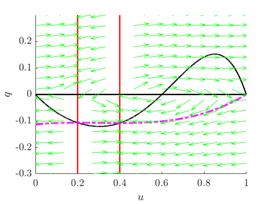
An implicit solution to equation (1) with (40) and (2) can be constructed using the nonclassical symmetry described in Section 1. Figures 10(c) and 10(d) show a receding travelling wave solution. The dashed line in panel (d) indicates the difference in shock location as chosen by the requirement that $\Phi^{\prime}(u)$ is continuous and the equal area rule.

4 Discussion and conclusion

Analysis of nonlinear reaction–diffusion equations has wide-ranging application in the physical sciences. Nonclassical symmetry analysis can recover analytic solutions for specific diffusivity and reaction terms, including where diffusivity is negative. Negative diffusivity provides a phenomenological description of aggregation, and also arises in the continuum limit of discrete models with aggregation. We analyse analytic solutions to a reaction–diffusion equation with nonlinear diffusivity that is negative for some values of the density. These solutions are multi-valued, requiring the insertion of shock discontinuities. The combination of negative diffusivity and shock-fronted analytic solutions provides rich opportunities for analysis, which we explore in this work.

Exact solutions to nonlinear partial differential equations are rare. A major advantage of nonclassical symmetry techniques is their ability to uncover time-dependent exact solutions. A disadvantage of constructing solutions using a nonclassical symmetry is that we cannot impose an arbitrary initial condition. Instead, we identify the initial condition with the density profile of the symmetry solution at time $t=0.$ Owing to this limitation, we focus on the construction and analysis of exact symmetry solutions in this work. Furthermore, the connection between nonlinear reaction–diffusion equations with negative diffusivity and aggregation phenomena in a physical or biological system remains to be investigated. Consequently, we do not specify or solve a biologically-relevant initial-value problem for the reaction–diffusion equation with negative diffusivity in this work. Although preliminary numerical investigations using finite-difference and finite-volume methods yield solutions reminiscent of the shock-fronted solutions presented here, we do not focus on the numerical treatment of 1 further.

We consider three types of analytic solutions — a receding time-dependent solution, colliding waves, and receding travelling waves. These solutions are all sharp-fronted, such that the density $u=0$ at some $x=L(t)$ with $u^{\prime}(L(t),t)\neq 0.$ In all solutions, the boundary $L(t)$ evolves according to a Stefan-like condition. We insert shocks in the density profile to resolve regions where $u(x,t)$ is multi-valued. We place shocks such that the flux potential $\Phi(u)$ and its derivative $\Phi^{\prime}(u)$ are continuous across the shock. For diffusivity that is symmetric about the midpoint of its zeros (e.g. the quadratic 6), these conditions are equivalent to the more commonly-used equal-area rule. With symmetric diffusivity, the continuity and equal-area requirements recover the shock with longest possible length. For a non-symmetric diffusivity, the largest jump coincides with the continuity condition only. Since another way to write equation 1 is equation 8, the requirement that $\Phi^{\prime}(u)$ is continuous has stronger foundation than imposing equal-area. Our planned future investigation of the entropy jump across the shock and regularisation to the PDE might yield further understanding about the link between negative diffusivity and physical phenomena.

The solutions presented here avoid the values of $u(x,t)$ for which the diffusivity becomes negative. It is interesting then that the solutions do not display the usual characteristics of a standard diffusion model. This may be a consequence of the loss of mass at the moving boundary, although it is more likely that the negative values of $D(u)$ impact the solution despite the solution not taking on the relevant values of $u$ . While the travelling wave solutions presented are exact solutions that satisfy the PDE, they are not weak solutions in the usual sense of averaging through the PDE with an arbitrary compactly-supported test function. We refer the reader to Whitham [39] for further information about weak solutions that contain shocks.

In addition to presenting the analytic solutions, we perform spectral stability analysis for constant and travelling wave solutions. We show that the constant solution $u=0$ is stable, but that $u=1$ admits long-wavelength instability for quadratic diffusivity with $a+b>1.$ We also prove spectral stability of travelling wave solutions to 1 with quadratic diffusivity 6, for some combinations of $a$ and $b.$ However, open problems remain in the analysis of analytic solutions to reaction–diffusion equations with negative diffusivity. For non-symmetric diffusivity, the continuity of flux $\Phi(u)$ and its derivative $\Phi^{\prime}(u)$ conditions for defining shocks do not yield an equal-area rule. The regularisation to the nonlinear reaction–diffusion equation 1 corresponding to the requirement for $\Phi^{\prime}(u)$ to be continuous remains unknown. Investigation of this and other regularisations will be the subject of future work, as will a study of the jump in entropy across the shock.

Acknowledgements

This work was supported by the Australian Research Council Discovery Program (grant numbers DP200102130 and DP230100406).

References

Alt [1985] W. Alt. Models for mutual attraction and aggregation of motile individuals. In V. Capasso, E. Grosso, and S. L. Paveri-Fontana, editors, Mathematics in Biology and Medicine, pages 33–38, Berlin, Heidelberg, 1985. Springer Berlin Heidelberg.
Aronson [1985] D. G. Aronson. The role of diffusion in mathematical population biology: Skellam revisited. In V. Capasso, E. Grosso, and S. L. Paveri-Fontana, editors, Mathematics in Biology and Medicine, pages 2–6, Berlin, Heidelberg, 1985. Springer Berlin Heidelberg.
Arrigo and Hill [1995] D. J. Arrigo and J. M. Hill. Nonclassical symmetries for nonlinear diffusion and absorption. Studies in Applied Mathematics, 94(1):21–39, 1995.
Bluman and Cole [1969] G. W. Bluman and J. D. Cole. The general similarity solution of the heat equation. Journal of Mathematics and Mechanics, 18(11):1025–1042, 1969.
Bradshaw-Hajek et al. [2023] B. H. Bradshaw-Hajek, I. Lizarraga, R. Marangell, and M. Wechselberger. A geometric singular perturbation analysis of generalised shock selection rules in reaction-nonlinear diffusion models. arXiv preprint arXiv:2308.02719, 2023.
Broadbridge et al. [2002] P. Broadbridge, B. H. Bradshaw, G. R. Fulford, and G. K. Aldis. Huxley and Fisher equations for gene propagation: An exact solution. The Anziam Journal, 44(1):11–20, 2002.
Broadbridge et al. [2023] P. Broadbridge, B. H. Bradshaw-Hajek, and A. J. Hutchinson. Conditionally integrable pdes, nonclassical symmetries and applications. Proceedings of the Royal Society A, 479(2276):20230209, 2023.
Courchamp et al. [1999] F. Courchamp, T. Clutton-Brock, and B. Grenfell. Inverse density dependence and the Allee effect. Trends in Ecology & Evolution, 14(10):405–410, 1999.
Du and Lin [2010] Y. Du and Z. Lin. Spreading-vanishing dichotomy in the diffusive logistic model with a free boundary. SIAM Journal on Mathematical Analysis, 42(1):377–405, 2010.
Edwards et al. [2018] M. P. Edwards, B. H. Bradshaw-Hajek, M. J. Munoz-Lopez, P. M. Waterhouse, and R. S. Anderssen. Compactly supported solutions of reaction–diffusion models of biological spread. In Agriculture as a Metaphor for Creativity in All Human Endeavors, pages 125–138. Springer, 2018.
El-Hachem et al. [2019] M. El-Hachem, S. W. McCue, W. Jin, Y. Du, and M. J. Simpson. Revisiting the Fisher–Kolmogorov–Petrovsky–Piskunov equation to interpret the spreading–extinction dichotomy. Proceedings of the Royal Society A: Mathematical, Physical and Engineering Sciences, 475(2229):20190378, 2019.
El-Hachem et al. [2021] M. El-Hachem, S. W. McCue, and M. J. Simpson. Invading and receding sharp-fronted travelling waves. Bulletin of Mathematical Biology, 83(4):1–25, 2021.
Fadai [2021] N. T. Fadai. Semi-infinite travelling waves arising in a general reaction–diffusion Stefan model. Nonlinearity, 34(2):725–743, 2021. ISSN 0951-7715. doi: 10.1088/1361-6544/abd07b.
Ferracuti et al. [2009] L. Ferracuti, C. Marcelli, and F. Papalini. Travelling waves in some reaction-diffusion-aggregation models. Advances in Dynamical Systems and Applications, 4(1):19–33, 2009.
Goard [2008] J. Goard. Finding symmetries by incorporating initial conditions as side conditions. European Journal of Applied Mathematics, 19(6):701–715, Dec. 2008. ISSN 0956-7925, 1469-4425. doi: 10.1017/S0956792508007705.
Goard and Broadbridge [1996] J. Goard and P. Broadbridge. Nonclassical symmetry analysis of nonlinear reaction-diffusion equations in two spatial dimensions. Nonlinear Analysis: Theory, Methods & Applications, 26(4):735–754, 1996.
Grünbaum and Okubo [1994] D. Grünbaum and A. Okubo. Modelling social animal aggregations. In S. A. Levin, editor, Frontiers in Mathematical Biology, pages 296–325, Berlin, Heidelberg, 1994. Springer Berlin Heidelberg.
Harley et al. [2014] K. Harley, P. van Heijster, R. Marangell, G. J. Pettet, and M. Wechselberger. Existence of traveling wave solutions for a model of tumor invasion. SIAM Journal on Applied Dynamical Systems, 13(1):366–396, 2014.
Ibragimov [1999] N. H. Ibragimov. Elementary Lie group analysis and ordinary differential equations, volume 197. Wiley New York, 1999.
Johnston et al. [2017] S. T. Johnston, R. E. Baker, D. L. S. McElwain, and M. J. Simpson. Co-operation, competition and crowding: a discrete framework linking Allee kinetics, nonlinear diffusion, shocks and sharp-fronted travelling waves. Scientific Reports, 7(1):1–19, 2017.
Kapitula and Promislow [2013] T. Kapitula and K. Promislow. Spectral and dynamical stability of nonlinear waves, volume 457. Springer, 2013.
Keller and Segel [1970] E. F. Keller and L. A. Segel. Initiation of slime mold aggregation viewed as an instability. J. Theor. Biol., 26(3):399–415, 1970. ISSN 0022-5193. doi: 10.1016/0022-5193(70)90092-5.
Kuzmin and Ruggerini [2011] M. Kuzmin and S. Ruggerini. Front propagation in diffusion-aggregation models with bi-stable reaction. Discrete & Continuous Dynamical Systems — B, 16(3):819–833, 2011.
Lewis and Kareiva [1993] M. A. Lewis and P. Kareiva. Allee dynamics and the spread of invading organisms. Theoretical Population Biology, 43(2):141–158, 1993.
Li et al. [2020] Y. Li, P. van Heijster, R. Marangell, and M. J. Simpson. Travelling wave solutions in a negative nonlinear diffusion–reaction model. Journal of Mathematical Biology, 81(6-7):1495–1522, 2020.
Li et al. [2021] Y. Li, P. van Heijster, M. J. Simpson, and M. Wechselberger. Shock-fronted travelling waves in a reaction–diffusion model with nonlinear forward–backward–forward diffusion. Physica D: Nonlinear Phenomena, 423:132916, 2021.
Lie [1880] S. Lie. Theorie der transformationsgruppen I. Mathematische Annalen, 16(4):441–528, 1880.
Lundberg and Totik [2013] E. Lundberg and V. Totik. Lemniscate growth. Anal. Math. Phys., 3(1):45–62, 2013. doi: 10.1007/s13324-012-0038-1.
Maini et al. [2006] P. K. Maini, L. Malaguti, C. Marcelli, and S. Matucci. Diffusion-aggregation processes with mono-stable reaction terms. Discrete & Continuous Dynamical Systems — B, 6(5):1175–1189, 2006.
Moitsheki et al. [2005] R. J. Moitsheki, P. Broadbridge, and M. P. Edwards. Symmetry solutions for transient solute transport in unsaturated soils with realistic water profile. Transport in Porous Media, 61:109–125, 2005.
Olver [2000] P. J. Olver. Applications of Lie groups to differential equations, volume 107. Springer Science & Business Media, 2000.
Pego [1989] R. L. Pego. Front migration in the nonlinear Cahn-Hilliard equation. Proceedings of the Royal Society of London. A. Mathematical and Physical Sciences, 422(1863):261–278, 1989.
Pettet et al. [2000] G. J. Pettet, D. L. S. McElwain, and J. Norbury. Lotka-Volterra equations with chemotaxis: walls, barriers and travelling waves. Mathematical Medicine and Biology: A Journal of the IMA, 17(4):395–413, 2000.
Popescu and Dietrich [2004] M. N. Popescu and S. Dietrich. Model for spreading of liquid monolayers. Physical Review E, 69(6):061602, 2004.
Sherratt and Murray [1990] J. A. Sherratt and J. D. Murray. Models of epidermal wound healing. Proceedings of the Royal Society of London. Series B: Biological Sciences, 241(1300):29–36, 1990.
Stephens and Sutherland [1999] P. A. Stephens and W. J. Sutherland. Consequences of the Allee effect for behaviour, ecology and conservation. Trends in ecology & evolution, 14(10):401–405, 1999.
Turchin [1989] P. Turchin. Population consequences of aggregative movement. Journal of Animal Ecology, 58(1):75–100, 1989.
Wechselberger and Pettet [2010] M. Wechselberger and G. J. Pettet. Folds, canards and shocks in advection–reaction–diffusion models. Nonlinearity, 23(8):1949, 2010.
Whitham [2011] G. B. Whitham. Linear and nonlinear waves. John Wiley & Sons, 2011.
Witelski [1995] T. P. Witelski. Shocks in nonlinear diffusion. Applied Mathematics Letters, 8(5):27–32, 1995.
Witelski [1996] T. P. Witelski. The structure of internal layers for unstable nonlinear diffusion equations. Studies in Applied Mathematics, 97(3):277–300, 1996.