remarkRemark \newsiamremarkhypothesisHypothesis \newsiamremarkexampleExample \newsiamthmassumptionAssumption \newsiamthmclaimClaim \headersConvergence of SALS for Random TensorsY. Cao, S. Das, L. Oeding, H.-W. van Wyk
Analysis of the Stochastic Alternating Least Squares Method for the Decomposition of Random Tensors††thanks: Submitted to the editors 04/01/2020.
Abstract
Stochastic Alternating Least Squares (SALS) is a method that approximates the canonical decomposition of averages of sampled random tensors. Its simplicity and efficient memory usage make SALS an ideal tool for decomposing tensors in an online setting. We show, under mild regularization and readily verifiable assumptions on the boundedness of the data, that the SALS algorithm is globally convergent. Numerical experiments validate our theoretical findings and demonstrate the algorithm’s performance and complexity.
keywords:
canonical decomposition, parallel factors, stochastic optimization, stochastic alternating least squares, random tensor, block nonlinear Gauss-Seidel65K10, 90C15, 15A69, 68W20
1 Introduction
Multi-modal data is represented by a tensor, or a multidimensional matrix. Tensor data is present in ares such as Natural Language Processing (NLP) [8], Blind Source Separation (BSS) [9, 28], and Phylogenetic Tree Reconstruction (PTR) [12, 2, 17]. In each of these areas, canonical decomposition (CANDECOMP)/parallel factors (PARAFAC), also known as CP tensor decomposition (representing a given tensor as a sum of rank-one tensors), provides important insights since the components of the rank-one terms, the factors, represent meaning in the data. For NLP given a tensor constructed from large text databases, the rank-one terms could represent topics, and the factors could represent words. For BSS given a tensor constructed from signals arriving at a single receiver from unknown sources, the rank-one terms could represent sources, and the factors could be used to locate the sources. For PTR given a tensor constructed as a contingency table for instances of neucleotide combinations from aligned DNA from several species, the factors represent model parameters for the phylogenetic tree.
In applications observations may represent samples of an underlying random tensor. For example, the word co-occurence frequencies used in NLP may come from a sample of a collection of documents. Here fast, reliable algorithms are desired for the CP decomposition of the average tensor. Because CP decomposition is known to be NP hard in general [15], and because the average tensor is usually only available through sampling, we investigate approximate decompositions based on stochastic optimization. In [22], Maehara et al. propose a stochastic version of the widely-used alternating least squares (ALS) method, the stochastic alternating least squares (SALS) method, and show the algorithm’s efficiency by means of numerical experiments. In this paper, we provide a detailed analysis of the algorithm, showing under mild regularization and a minimal set of verifiable assumptions that it is globally convergent to a local minimizer for any initial guess. In Section 4, we also include a detailed discussion the algorithm’s complexity and efficiency.
The alternating least squares (ALS) method, first proposed by Carroll and Chang [10], remains the most widely used algorithm for computing the CP decomposition of a tensor [13]. This block-nonlinear Gauss-Seidel method [5, 26] exploits the component-wise quadratic structure of the cost functional to compute iterates efficiently and with a low memory footprint. It has been modified [11] to exploit sparsity structure in data, which typically occurs in tensors representing co-occurence frequencies such as in the tree reconstruction above. Regularized versions of the ALS method, as well as the associated proximal minimization iterations considered in [21], help mitigate the potential ill-posedness of the CP problem to within sample noise. Although one may compute the tensor’s expectation a priori and decompose it by means of the standard ALS method (see Remark 2.1), such an approach results in a loss of sparsity and cannot seemlessly acommodate the arrival of new samples. In [22], Maehara et al. proposed the Stochastic Alternating Least Squares method, a block-stochastic minimization method that preserves the salient features of the ALS method, while also efficiently incorporating tensor samples in the optimization procedure. Recent work (see [3, 20]) has considered the related problem of using randomized (or stochastic) methods to decompose existing large-scale tensors. In particular, in [3], a variant of the ALS method is developed that approximates the component least squares problem efficiently by randomized/sketching methods. In [20], a dense tensor is expressed as the expectation of a sequence of sparse ones, thereby allowing the use of stochastic gradient descent (SGD) methods.
The convergence analysis of the SALS algorithm applied to the CP decomposition of a random tensor is complicated by the fact that the underlying cost functional is not convex. Moreover, the algorithm itself is a stochastic, block-iterative, second order method whose successive iterates do not have the Markovian dependence structure present in classical stochastic gradient descent (SGD) methods. The convergence of the ALS method was studied in [6], where a quotient-linear convergence rate was established. Block-coordinate techniques for the unconstrained optimization of general, possibly nonconvex, deterministic functionals were treated in [14] (see also [25, 4, 32] and references therein). Xu and Yin [31] discuss the convergence of block stochastic gradient methods for averages of convex and nonconvex functionals. They rely on assumptions (such as the uniformly bounded variance of gradient iterates) that, while standard in the literature (see e.g. [7]), are difficult to verify in practice since they pertain to the algorithm itself. The main contributions of this paper are to prove the convergence of the SALS algorithm, a block-stochastic Newton method, for the CP decomposition of the average of a random tensor, subject to a single verifiable assumption relating to the boundedness of the observed data.
This paper is structured as follows. In Section 2, we introduce the CP decomposition problem for random tensors and describe the stochastic alternating least squares algorithm (Algorithm 2). Section 3 contains our main theoretical contributions. In Section 3.1, we exploit the special multinomial structure of the cost functional to quantify the regularity of its component-wise gradient and Hessian in terms of the size of the algorithm’s iterate vectors (see Lemma 3.5 and its corollaries). In Section 3.2 we show that the iterates themselves can be bounded in terms of the random tensor to be decomposed (Lemma 3.15), which naturally leads to our single, verifiable assumption on the latter’s statistical properties (3.16). In Section 3.3, we show that the iterates generated by the SALS algorithm converge to a local minimizer. We validate the SALS method numerically via a few computational examples in Section 4 and offer concluding remarks in Section 5.
2 Notation and Problem Description
We to follow notational conventions that are closely aligned with the literature on the CP decomposition (see [19]), as well as on stochastic optimization (see [7, 31]). Use use lower case letters to denote scalars, bold letters for vectors, uppercase letters for matrices, and uppercase calligraphic letters for tensors. We use superscripts to indicate iteration (or sub-iteration) indices and subscripts for components, i.e. is the -th component at the -th iteration. Multi-indices are denoted by bold letters and sums, products, and integrals over these should be interpreted to be in iterated form. For the block coordinate minimization method in Algorithm 2, it is convenient to express the vector in terms of its -th block component and the remaining components, denoted . Using this notation, we write with the implicit understanding that the block components are in the correct order. The Frobenius norm of a vector, matrix, or tensor, i.e. the root mean square of its entries, is denoted by . For , denotes the standard Euclidean -norm for vectors and the induced matrix -norm for matrices. We use ‘’ to denote the outer product, ‘’ for the component-wise (or Hadamard) product, ‘’ for the column-wise Khatri-Rao product, and ‘’ for the Kronecker product.
Let be a complete probability space and let be a measurable map, also known as a -th order random tensor. In practice the underlying probability space is rarely known explicitly. Instead, its law can often be observed indirectly through sample realizations of that are assumed to be independent and identically distributed (iid). We use to denote expectation:
for any integrable function .
The rank- decomposition problem for (or its sample realizations) amounts to finding a set of rank-one deterministic tensors , so that the quantity
| (1) |
is a good overall representation of . Each rank-one tensor , , is formed by the outer product where for each , i.e. is defined component-wise by
We use the mean squared error to measure the quality of the representation. Other risk measures may be more appropriate, depending on the application, possibly requiring a different analysis and approximation technique.
For analysis and computation, it is convenient to consider two other representations of the design variable. We define the -th factor matrix in to consist of the -th component vectors of each term in decomposition (1). Let , with , be the vectorization of the factor matrices, i.e. the concatenation of their column vectors. We also write in block component form as , where for . To emphasize dependence of on , we write the following (which also defines )
No efficient closed form solution of the factorization problem exists (even for deterministic tensors) [15]. So it is commonly reformulated as the optimization problem
| (2) |
Remark 2.1.
Letting and , it follows readily that
Since the variance of is constant in the design variable , the minimization Problem (2) is equivalent to the decomposition of the expected tensor, i.e.
The analysis in this work is however based on the formulation given by (2), since it lends itself more readily to extensions to more general risk functions.
Tensor decompositions have scale ambiguity. Indeed, for any direction and any scalars , let . Then
The optimizer of (2) therefore lies on a simply connected manifold (see [30]), which can lead to difficulties in the convergence of optimization algorithms. To ensure isolated minima that can be readily located, it is common to enforce bounds on the size of the factors, either directly through an appropriate normalization (see [30]), or indirectly through the addition of a regularization term [22]. We pursue the latter strategy, leading to the problem
| (3) |
While the regularization term biases the minimizers of Problem (2) its inclusion is key to guaranteeing well-posedness in the presence of noise. It plays a pivotal role in (i) proving the existence of a minimizer (Lemma 2.2), (ii) ensuring the positive-definiteness of the Hessian (Corollary 3.11), and (iii) guaranteeing the boundedness of iterates in terms of random tensor (Lemma 3.15). Heuristic methods are typically used to choose the value of that balances the bias of the optimizers against stability considerations, the most well-known of which is the Morozov discrepancy principle [24].
Lemma 2.2 (Existence of Minimizers).
Problem (3) has at least one minimizer.
Proof 2.3.
Let . So there exists a sequence in with
from which it follows that is bounded. The inequality
| (4) |
allows us to establish the boundedness of . By compactness, there exists a convergent subsequence as . The continuity of then implies
Remark 2.4.
2.1 The Stochastic Alternating Least Squares Method
Although the objective function is a high degree polynomial in general, it is quadratic in each component factor matrix . This is apparent from the matricized form of (3). Recall [18] that the columnwise Khatri-Rao product of matrices and is defined as their columnwise Kronecker product, i.e. . The matricization of the rank tensor along the -th fiber takes the form (see [1])
| (6) |
where is defined to be the iterated Khatri-Rao product on the right. Note that does not depend on , and hence the matricized tensor decomposition is linear in . Since the Frobenius norm is invariant under matricization, the sample objective function can then be rewritten as a quadratic function in , i.e.
Vectorizing this form yields a linear least squares objective function in , namely
whose component-wise gradient and Hessian are given respectively by
| (7) | ||||
| (8) |
where and are identity matrices. In the presence of regularization, the Hessian matrix (8) is strictly positive definite with lower bound that is independent of both and of the remaining components (see Corollary 3.11). Consequently, each sampled component-wise problem
has a unique solution given by the stationary point satisfying . It is more efficient to use the matricized form of the stationarity condition, i.e.
| (9) |
For any , it can be shown [29] that
where denotes the (Hadamard) product. Repeatedly using this identity, we have
| (10) |
so the Hessian can be computed as the component-wise product of matrices in .
The (deterministic) ALS method (Algorithm 1) exploits the component-wise quadratic structure of the objective functional , which it inherits from . In the -th block iteration, the ALS algorithm cycles through the components of , updating each component in turn in the direction of the component-wise minimizer. The function is also updated at each subiteration to reflect this change. Specifically, the iterate at the beginning of the -th block is denoted by
The ALS algorithm then generates a sequence of sub-iterates , where
Note that, under this convention, .
Although the descent achieved by the ALS method during -th block iteration is most likely not as large as a descent would be for a monolithic descent direction for over the entire space , the ALS updates can be obtained at a significantly lower computational cost and with a lower memory footprint.
The block-component-wise quadratic structure of the integrand allows us to compute explicitly. To this end we form the second order Taylor expansion about at the current iterate , i.e.
| (11) | ||||
Note that does not depend explicitly on and is therefore a deterministic quantity for known . The component-wise minimizer of can be calculated explicitly as the Newton update
Although both the design variable and the functions appearing in Problem (3) are deterministic, any gradient based optimization procedure, such as the ALS method described above, requires the approximation of an expectation at every iterate, the computational effort of which is considerable. This suggests the use of stochastic gradient sampling algorithms that efficiently incorporate the sampling procedure into the optimization iteration, while exploiting data sparsity.
The stochastic gradient descent method [27] addresses the cost of approximating the expectation by computing descent directions from small sampled batches of function values and gradients at each step of the iteration. To accommodate the noisy gradients, the step size is reduced at a predetermined rate. For the stochastic alternating least squares (SALS) method (Algorithm 2), we determine the sample at the beginning of the -th block iteration. For a batch of iid random samples of , we write the component-wise batch average of as
As before, we can compute the component-wise minimizer
| (12) |
at the -th subiteration by means of the Newton step. To this end we express in terms of its second order Taylor expansion about the current iterate , i.e.
The sample minimizer is thus
To mitigate the effects of noise on the estimate, especially during later iterations, we modify the update by introducing a variable stepsize parameter , so that
| (13) |
It is well known (see e.g. [7]) that a stepsize that decreases at the rate of as leads to an optimal convergence rate for stochastic gradient methods. Here, we specify that the stepsize takes the form , where is a strictly positive, bounded sequence, i.e. there are constants such that
One of the difficulties in analyzing the convergence behavior of stochastic sampling methods arises from the fact that the iterates constitute a stochastic process generated by a stochastic algorithm that depends on the realizations of the sample batches . Consequently, even deterministic functions, such as , become stochastic when evaluated at these points, e.g. is a random quantity. Moreover, successive iterates are statistically dependent, since later iterates are updates of earlier ones. Specifically, let be the -algebra generated by the first sample batches. At the end of the -th subiteration in the -th block, the first components of have been updated using and are thus -measurable, whereas the remaining components depend only on and are therefore only -measurable. To separate the effect of from that of on an -measurable random variable , it is often useful to invoke the law of total expectation, i.e.
3 Convergence Analysis
Here we discuss the convergence of Algorithm 2. Since Problem (3) is nonconvex, there can in general be no unique global minimizer. Theorem 3.25 establishes the convergence of the SALS iterates to a local minimizer in expectation. Yet, the special structure of the CP problem allows us to forego most of the standard assumptions made in the SGD framework. In fact, we only assume boundedness of the sampled data . Indeed, we show that the regularity of the component-wise problem, as the Lipschitz constant of the gradient, depends only on the norm of the current iterate , which is in turn bounded by (Lemma 3.15).
3.1 Regularity Estimates
In the following we exploit the multinomial structure of the cost functional to establish component-wise regularity estimates, such as local Lipschitz continuity of the sampled gradient and of the Newton step , as well as bounded invertibility of the Hessian .
In the proofs below, we will often need to bound a sum of the form in terms of , where . For this we use the fact that for finite dimensional vector spaces all norms are equivalent. In particular, for any norm subscripts and , there exist dimension-dependent constants so that
| (14) |
Using norm equivalence with and , we obtain
| (15) |
where , while and are the appropriate constants in the norm equivalence relation above for and respectively.
The estimates established in this section all follow from the local Lipschitz continuity of the mapping , shown in Lemma 3.1 below.
Lemma 3.1.
Proof 3.2.
First note that for any , properties of Kronecker products, the Cauchy-Schwartz inequality, and Inequality (15) imply that
| (17) |
Let denote the indices in the Khatri-Rao product (6). Addition and subtraction of the appropriate cross-terms provides
By (17), each term in the sum above can be bounded in norm by
In the special case when , Inequality (16) reduces to
| (18) |
Corollary 3.3.
Proof 3.4.
By the equivalence of the induced Euclidean and the Frobenius norms,
Letting in (19), yields the bound
| (21) |
As a first consequence of Lemma 3.1 and Corollary 3.3, we can obtain an explicit form for the component-wise Lipschitz constant of .
Lemma 3.5.
Proof 3.6.
Let and be constructed from and respectively via Equation Eq. 6. Using Eq. 7, the difference in sampled component-wise gradients is given by
The following is a simplified upper bound in the special case when and only differ in their -th block components
Corollary 3.7.
For any , we have
| (24) |
Proof 3.8.
We may also bound the norm of the component-wise gradient in terms of the norm of and the data , as shown in the following corollary.
Corollary 3.9.
Corollary 3.3 also implies the following bounds on the component-wise Hessian.
Corollary 3.11.
For any and ,
| (26) |
Proof 3.12.
This follows directly from the fact that
Finally, we establish the local Lipschitz continuity of the Newton step mapping .
Proof 3.14.
3.2 Boundedness of the Data
In this section we bound the norm of the component iterates in terms of the norm of the initial guess and maximum value of the sequence of sample averages of the norms of .
Lemma 3.15.
Proof 3.16.
Since the regularity estimates derived above all involve powers of and of , Lemma 3.15 suggests that a bound on the data is sufficient to guarantee the regularity of the cost functional, gradient, and Newton steps that are necessary to show convergence. In the following we assume such a bound and pursue its consequences.
[Bounded data] There is a constant so that
| (30) |
Remark 3.17.
This assumption might conceivably be weakened to one pertaining to the statistical distribution of the maxima . Specifically, letting , it can be shown under appropriate conditions on the density of , that converges in distribution to a random variable with known extreme value density. The analysis below will hold if it can be guaranteed that the limiting distribution has bounded moments of sufficiently high order. This possibility will be pursued in future work.
An immediate consequence of 3.16 is the existence of a uniform bound on the radius and hence on the iterates .
Corollary 3.18.
Given 3.16, there exist finite, non-negative constants , and independent of and of , so that for all ,
| (31) | ||||
| (32) | ||||
| (33) |
Proof 3.19.
3.3 Convergence
We now consider the difference between the sampled and expected search directions. For the standard stochastic gradient descent algorithm, this stochastic quantity vanishes in expectation, given past information , i.e. , since is an unbiased estimator of . For the stochastic alternating least squares method, this is no longer the case. Lemma 3.20 however uses the regularity of the gradient and the Hessian to establish an upper bound that decreases on the order as .
Lemma 3.20.
There is a constant such that for every and ,
| (34) |
where .
Proof 3.21.
Recall that the current iterate is statistically dependent on sampled tensors , while its first components also depend on . For the purpose of computing , we suppose that are known and write to emphasize its dependence on . Thus
By definition, and since is an unbiased estimator of , we have
Moreover, since and are identically distributed,
Therefore
| (35) |
In the special case , the iterate , and hence , does not depend on . Since is an unbiased estimator of , we have
We now consider the case . Using the Lipschitz continuity of the mapping (Lemma 3.13), the bounds in Corollary 3.18, and Jensen’s inequality, we obtain
the integrand of which can be bounded by
The result now follows from taking expectations and using (27) with , in conjunction with (31), and (33).
Lemma 3.22.
If is -measurable and then
| (36) |
Proof 3.23.
The main convergence theorem is based on the following lemma (for a proof, see e.g. Lemma A.5, [23])
Lemma 3.24.
Let and be any two nonnegative, real sequences so that (i) , (ii) , and (iii) there is a constant so that for . Then .
Theorem 3.25.
Let be the sequence generated by the Stochastic Alternating Least Squares (SALS) method outlined in Algorithm 2. Then
Proof 3.26.
We base the proof on Lemma 3.24 with and . Clearly, Condition (i) in Lemma 3.24 is satisfied. To show that Condition (ii) holds, i.e. that for , we use the component-wise Taylor expansion (11) of the expected cost centered at the iterate and the SALS update given in (13) to express the expected decrease as
Since, by (32) and Corollary (3.11),
where , the above expression can be rearranged as
| (37) | ||||
Evidently, Condition (ii) of Lemma 3.24 holds as long as for . For a fixed , the first term generates a telescoping sum so that
| (38) |
since . Consider
Since is -measurable, Lemma 3.22 implies that the expectation of the second term can be bounded as follows
where by Corollaries 3.9 and 3.18. The first term satisfies
where by Lemmas 3.5 and 3.18. Combining these two bounds yields
| (39) |
Finally, we use Corollaries 3.9, 3.11, and 3.18 to bound
so that
| (40) |
By virtue of Inequality (37), the upper bounds (38), (39), and (40) now imply that Condition (ii) of Lemma 3.24 holds. It now remains to show that Condition (iii) of Lemma 3.24 holds, i.e. that as for all . By the reverse triangle inequality and by the Lipshitz continuity and boundedness of the gradient,
4 Numerical Experiments
In this section we detail the implementation of the SALS algorithm, discuss its computational complexity and perform a variety of numerical experiments to explore its properties and validate our theoretical results.
We invoke the matricized form (9) of the component-wise minimization problem for the sake of computational and storage efficiency. In particular, at the -th block iterate, we compute the sample/batch tensor average . Cycling through each component , we then compute the component-wise minimizer as the stationary matrix satisfying the matrix equation
| (41) |
Finally, we update the -th component factor matrix using the relaxation step
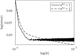
In all our numerical experiments, we use step sizes of the form , i.e. for and .
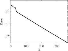
Example 4.1 (Convergence).
In our first example, we apply the SALS algorithm to a 3-dimensional random tensor of size constructed from a deterministic tensor with known decomposition. We generate random samples by perturbing each entry of with a uniformly distributed noise . We measured the accuracy at each step via the residual which can be computed exactly, since and are known. Figure 1 shows that when the noise parameter is zero and the stepsize rule is constant, we recover the quotient-linear performance of the regularized ALS method. In the presence of noise, however, the convergence rate decreases.
Computational Complexity
The computational effort of each block iteration of the SALS algorithm is determined by the cost of forming and solving Equation (41) for each component. Recall that is the specified rank, the tensor’s dimension, and where is the size of the -th vector component of each outer product in the expansion. Further, let be the total number of entries in and be the number of non-zero entries in . It can then readily be seen that the cost of forming the coefficient matrix is , that of computing the matricized tensor times Khatri-Rao product (MTTKRP) is , and that of solving the resulting dense symmetric system is . If , the computational cost of the MTTKRP dominates, especially as the density of increases and hence .
It is often claimed that single-sample stochastic gradient methods, i.e. those using for , make more efficient use of samples than their batch counterparts, i.e. for . Below, we investigate this claim for the SALS method. For simplicity assume that each sample tensor has a fixed fraction of zero entries, so that . Barring cancellation and assuming a uniform, independent distribution of nonzero entries, we estimate , where is the sample size. Adding the cost of forming the average then gives the computational cost of each block iteration as
| (42) |
To compare the asymptotic efficiency of the single-sample SALS method with that of a batch method, we fix a computational budget and investigate the estimated error achieved by each approach. Note that once is fixed, the number of iterations is determined by the budget as . We first consider the case and let be the overall minimizer. If we assume the convergence rate to be sublinear, i.e. the error satisfies
then the accuracy of the SALS method with a budget of is on the order of
| (43) |
Now suppose . To obtain the best possible accuracy of the batch ALS methods (with budget ) requires the optimal combination of batch size and number of iterations . Let be the batch minimizer, where , and let be the terminal iterate. The overall error is given by,
Since , we can bound the error above by the sum of a sampling error and an optimization error . Assuming the asymptotic behavior of the sampling error to be and using the q-linear convergence rate for some of ALS (see [6]) as an optimistic estimate, the total error takes the form . Under the budget constraint, the error can thus be written as
| (44) |
For large, high-dimensional tensors the number of iterations allowable under the budget will decrease rapidly as grows, so that the second term dominates the optimal error in Equation (44), whereas smaller problems have an optimal error dominated by the Monte-Carlo sampling error .
Example 4.2 (Sparsity).
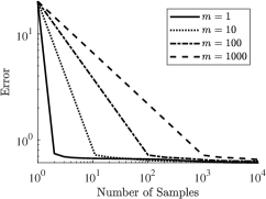
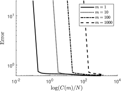
To compare the computational complexity of the single-sample SALS method, i.e. , with that of the batch SALS method, i.e. , we form a sequence of three-dimensional random sparse tensors with , , and and a fixed fraction of nonzero entries. For these tensors, the first and second moments are known and hence residuals can be computed accurately. In Fig. 2 we verify how an increase in the batch size deteriorates the sparsity of the tensor and lowers the sampling error at the predicted rate.
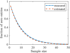
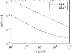
Figure 3 shows the efficiency of the SALS algorithm with batch sizes , and . To this end, we fixed a computational budget of 10k total samples and used this to determine the number of iteration steps based on the batch size . Clearly the SALS method that uses a single sample for each block iteration makes much more efficient use of samples than variants with larger batch sizes.
5 Conclusion
In this work, we showed that the SALS method is globally convergent and demonstrated the benefits of using stochastic-gradient-based approaches, especially in the decomposition of large, sparse tensors. In our analysis we focused on regularization in the Frobenius norm, and have not included a discussion on related proximal point algorithms or other regularization approaches (see e.g. [21, 30, 31]). Another interesting avenue of exploration relates to the choice of cost functional in tensor decomposition. Even though the quadratic structure afforded by the Frobenius norm is essential to the effectiveness of the ALS method, the standard statistical basis of comparison, namely expectation, could potentially be extended to other statistical metrics, such as those used in risk averse optimization methods. Finally, we foresee the application and extension of the SALS in the analysis and decomposition of real data sets.
References
- [1] E. Acar, D. M. Dunlavy, and T. G. Kolda, A scalable optimization approach for fitting canonical tensor decompositions, Journal of Chemometrics, 25 (2011), pp. 67–86.
- [2] E. S. Allman and J. A. Rhodes, The identifiability of tree topology for phylogenetic models, including covarion and mixture models, Journal of Computational Biology, 13 (2006), pp. 1101–1113.
- [3] C. Battaglino, G. Ballard, and T. G. Kolda, A practical randomized CP tensor decomposition, SIAM Journal on Matrix Analysis and Applications, 39 (2018), pp. 876–901.
- [4] A. Beck and L. Tetruashvili, On the convergence of block coordinate descent type methods, SIAM Journal on Optimization, 23 (2013), pp. 2037–2060.
- [5] D. P. Bertsekas and J. N. Tsitsiklis, Parallel and Distributed Computation: Numerical Methods, Prentice-Hall, Inc., USA, 1989.
- [6] J. C. Bezdek and R. J. Hathaway, Convergence of alternating optimization, Neural, Parallel Sci. Comput., 11 (2003), pp. 351–368.
- [7] L. Bottou, F. E. Curtis, and J. Nocedal, Optimization methods for large-scale machine learning, SIAM Review, 60 (2018), pp. 223–311.
- [8] G. Bouchard, J. Naradowsky, S. Riedel, T. Rocktäschel, and A. Vlachos, Matrix and tensor factorization methods for natural language processing, in Proceedings of the 53rd Annual Meeting of the Association for Computational Linguistics and the 7th International Joint Conference on Natural Language Processing: Tutorial Abstracts, Beijing, China, July 2015, Association for Computational Linguistics, pp. 16–18.
- [9] M. Boussé, O. Debals, and L. De Lathauwer, A tensor-based method for large-scale blind source separation using segmentation, IEEE Transactions on Signal Processing, 65 (2017), pp. 346–358.
- [10] J. D. Carroll and J.-J. Chang, Analysis of individual differences in multidimensional scaling via an n-way generalization of “eckart-young” decomposition, Psychometrika, 35 (1970), pp. 283–319.
- [11] D. Cheng, R. Peng, I. Perros, and Y. Liu, Spals: Fast alternating least squares via implicit leverage scores sampling, in Proceedings of the 30th International Conference on Neural Information Processing Systems, NIPS’16, Red Hook, NY, USA, 2016, Curran Associates Inc., p. 721–729.
- [12] N. Eriksson, Algebraic statistics for computational biology, vol. 13, Cambridge University Press, 2005, ch. Tree construction using singular value decomposition, pp. 347–358.
- [13] N. K. M. Faber, R. Bro, and P. K. Hopke, Recent developments in CANDECOMP/PARAFAC algorithms: a critical review, Chemometrics and Intelligent Laboratory Systems, 65 (2003), pp. 119–137.
- [14] L. Grippo and M. Sciandrone, Globally convergent block-coordinate techniques for unconstrained optimization, Optimization Methods and Software, 10 (1999), pp. 587–637.
- [15] C. J. Hillar and L.-H. Lim, Most tensor problems are NP hard, J. ACM, 60 (2013). 0911.1393.
- [16] E. Hille and R. S. Phillips, Functional analysis and semi-groups, American Mathematical Society, Providence, R. I. Third printing of the revised edition of 1957, American Mathematical Society Colloquium Publications, Vol. XXXI.
- [17] M. Ishteva, H. Park, and L. Song, Unfolding latent tree structures using 4th order tensors, in International Conference on Machine Learning, 2013, pp. 316–324.
- [18] C. G. Khatri and C. R. Rao, Solutions to some functional equations and their applications to characterization of probability distributions, Sankhya: The Indian Journal of Statistics, Series A (1961-2002), 30 (1968), pp. 167–180.
- [19] T. G. Kolda and B. W. Bader, Tensor decompositions and applications, SIAM Review, 51 (2009), pp. 455–500.
- [20] T. G. Kolda and D. Hong, Stochastic gradients for large-scale tensor decomposition.
- [21] N. Li, S. Kindermann, and C. Navasca, Some convergence results on the regularized alternating least-squares method for tensor decomposition, Linear Algebra and its Applications, 438 (2013), pp. 796–812.
- [22] T. Maehara, K. Hayashi, and K.-i. Kawarabayashi, Expected tensor decomposition with stochastic gradient descent, in Proceedings of the Thirtieth AAAI Conference on Artificial Intelligence, AAAI’16, AAAI Press, 2016, pp. 1919–1925.
- [23] J. Mairal, Stochastic Majorization-Minimization Algorithms for Large-Scale Optimization, in NIPS 2013 - Advances in Neural Information Processing Systems, C. Burges, L. Bottou, M. Welling, Z. Ghahramani, and K. Weinberger, eds., Advances in Neural Information Processing Systems 26, South Lake Tahoe, United States, Dec. 2013, pp. 2283–2291.
- [24] V. A. Morozov, Methods for Solving Incorrectly Posed Problems, Springer New York, 1984.
- [25] Y. Nesterov, Efficiency of coordinate descent methods on huge-scale optimization problems, SIAM Journal on Optimization, 22 (2012), pp. 341–362.
- [26] J. M. Ortega and W. C. Rheinboldt, Iterative Solution of Nonlinear Equations in Several Variables, Society for Industrial and Applied Mathematics, jan 2000.
- [27] H. Robbins and S. Monro, A stochastic approximation method, The Annals of Mathematical Statistics, 22 (1951), pp. 400–407.
- [28] N. Sidiropoulos, G. Giannakis, and R. Bro, Blind PARAFAC receivers for DS-CDMA systems, IEEE Trans. on Signal Processing, 48 (2000), pp. 810–823.
- [29] A. Smilde, R. Bro, and P. Geladi, Multi-Way Analysis with Applications in the Chemical Sciences, John Wiley & Sons, Ltd, aug 2004.
- [30] A. Uschmajew, Local convergence of the alternating least squares algorithm for canonical tensor approximation, SIAM Journal on Matrix Analysis and Applications, 33 (2012), pp. 639–652.
- [31] Y. Xu and W. Yin, Block stochastic gradient iteration for convex and nonconvex optimization, SIAM Journal on Optimization, 25 (2015), pp. 1686–1716.
- [32] , A globally convergent algorithm for nonconvex optimization based on block coordinate update, Journal of Scientific Computing, 72 (2017), pp. 700–734.