This paper was converted on www.awesomepapers.org from LaTeX by an anonymous user.
Want to know more? Visit the Converter page.

Analysis and Design of Thompson Sampling
for Stochastic Partial Monitoring

Taira Tsuchiya
The University of Tokyo
RIKEN AIP
[email protected]
&Junya Honda
The University of Tokyo
RIKEN AIP
[email protected]
&Masashi Sugiyama
RIKEN AIP
The University of Tokyo
[email protected]
Abstract

We investigate finite stochastic partial monitoring, which is a general model for sequential learning with limited feedback. While Thompson sampling is one of the most promising algorithms on a variety of online decision-making problems, its properties for stochastic partial monitoring have not been theoretically investigated, and the existing algorithm relies on a heuristic approximation of the posterior distribution. To mitigate these problems, we present a novel Thompson-sampling-based algorithm, which enables us to exactly sample the target parameter from the posterior distribution. Besides, we prove that the new algorithm achieves the logarithmic problem-dependent expected pseudo-regret O(logT)\operatorname{O}(\log T) for a linearized variant of the problem with local observability. This result is the first regret bound of Thompson sampling for partial monitoring, which also becomes the first logarithmic regret bound of Thompson sampling for linear bandits.

1 Introduction

Partial monitoring (PM) is a general sequential decision-making problem with limited feedback (Rustichini, 1999; Piccolboni and Schindelhauer, 2001). PM is attracting broad interest because it includes a wide range of problems such as the multi-armed bandit problem (Lai and Robbins, 1985), a linear optimization problem with full or bandit feedback (Zinkevich, 2003; Dani et al., 2008), dynamic pricing (Kleinberg and Leighton, 2003), and label efficient prediction (Cesa-Bianchi et al., 2005).

A PM game can be seen as a sequential game that is played by two players: a learner and an opponent. At every round, the learner chooses an action, while the opponent chooses an outcome. Then, the learner suffers an unobserved loss and receives a feedback symbol, both of which are determined from the selected action and outcome. The main characteristic of this game is that the learner cannot directly observe the outcome and loss. The goal of the learner is to minimize his/her cumulative loss over all rounds. The performance of the learner is evaluated by the regret, which is defined as the difference between the cumulative losses of the learner and the optimal action (i.e., the action whose expected loss is the smallest).

There are mainly two types of PM games, which are the stochastic and adversarial settings (Piccolboni and Schindelhauer, 2001; Bartók et al., 2011). In the stochastic setting, the outcome at each round is determined from the opponent’s strategy, which is a probability vector over the opponent’s possible choices. On the other hand, in the adversarial setting, the outcomes are arbitrarily decided by the opponent. We refer to the PM game with finite actions and finite outcomes as a finite PM game. In this paper, we focus on the stochastic finite game.

One of the first algorithms for PM was considered by Piccolboni and Schindelhauer (2001). They proposed the FeedExp3 algorithm, the key idea of which is to use an unbiased estimator of the losses. They showed that the FeedExp3 algorithm attains O~(T3/4)\operatorname{\tilde{O}}(T^{3/4}) minimax regret for a certain class of PM games, and showed that any algorithm suffers linear minimax regret Ω(T)\Omega(T) for the other class. Here TT is the time horizon and the notation O~()\operatorname{\tilde{O}}(\cdot) hides polylogarithmic factors. The upper bound O~(T3/4)\operatorname{\tilde{O}}(T^{3/4}) is later improved by Cesa-Bianchi et al. (2006) to O(T2/3)\operatorname{O}(T^{2/3}), and they also provided a game with a matching lower bound.

In the seminal paper by Bartók et al. (2011), they classified PM games into four classes based on their minimax regrets. To be more specific, they classified games into trivial, easy, hard, and hopeless games, where their minimax regrets are 0, Θ~(T)\operatorname{\tilde{\Theta}}(\sqrt{T}), Θ(T2/3)\Theta(T^{2/3}), and Θ(T)\Theta(T), respectively. Note that the easy game is also called a locally observable game. After their work, several algorithms have been proposed for the finite PM problem (Bartók et al., 2012; Vanchinathan et al., 2014; Komiyama et al., 2015). For the problem-dependent regret analysis, Komiyama et al. (2015) proposed an algorithm that achieves O(logT)\operatorname{O}(\log T) regret with the optimal constant factor. However, it requires to solve a time-consuming optimization problem with infinitely many constraints at each round. In addition, this algorithm relies on the forced exploration to achieve the optimality, which makes the empirical performance near-optimal only after prohibitively many rounds, say, 10510^{5} or 10610^{6}.

Thompson sampling (TS, Thompson, 1933) is one of the most promising algorithms on a variety of online decision-making problems such as the multi-armed bandit (Lai and Robbins, 1985) and the linear bandit (Agrawal and Goyal, 2013b), and the effectiveness of TS has been investigated both empirically (Chapelle and Li, 2011) and theoretically (Kaufmann et al., 2012; Agrawal and Goyal, 2013a; Honda and Takemura, 2014). In the literature on PM, Vanchinathan et al. (2014) proposed a TS-based algorithm called BPM-TS (Bayes-update for PM based on TS) for stochastic PM, which empirically achieved state-of-the-art performance. Their algorithm uses Gaussian approximation to handle the complicated posterior distribution of the opponent’s strategy. However, this approximation is somewhat heuristic and can degrade the empirical performance due to the discrepancy from the exact posterior distribution. Furthermore, no theoretical guarantee is provided for BPM-TS.

Our goals are to establish a new TS-based algorithm for stochastic PM, which allows us to sample the opponent’s strategy parameter from the exact posterior distribution, and investigate whether the TS-based algorithm can achive sub-linear regret in stochastic PM. Using the accept-reject sampling, we propose a new TS-based algorithm for PM (TSPM), which is equipped with a numerical scheme to obtain a posterior sample from the complicated posterior distribution. We derive a logarithmic regret upper bound O(logT)\operatorname{O}(\log{T}) for the proposed algorithm on the locally observable game under a linearized variant of the problem. This is the first regret bound for TS on the locally observable game. Moreover, our setting includes the linear bandit problem and our result is also the first logarithmic expected regret bound of TS for the linear bandit, whereas a high-probability bound was provided, for example, in Agrawal and Goyal (2013b). Finally, we compare the performance of TSPM with existing algorithms in numerical experiments, and show that TSPM outperforms existing algorithms.

2 Preliminaries

This paper studies finite stochastic PM games (Bartók et al., 2011). A PM game with NN actions and MM outcomes is defined by a pair of a loss matrix 𝐋=(i,j)N×M\mathbf{L}=(\ell_{i,j})\in\mathbb{R}^{N\times M} and feedback matrix 𝐇=(hi,j)[A]N×M\mathbf{H}=(h_{i,j})\in[A]^{N\times M}, where AA is the number of feedback symbols and [A]={1,2,,A}[A]={\left\{1,2,\ldots,A\right\}}.

A PM game can be seen as a sequential game that is played by two players: the learner and the opponent. At each round t=1,2,,Tt=1,2,\dots,T, the learner selects action i(t)[N]i(t)\in[N], and at the same time the opponent selects an outcome based on the opponent’s strategy p𝒫Mp^{*}\in\mathcal{P}_{M}, where 𝒫n={pn:pk0,k=1npk=1}\mathcal{P}_{n}={\left\{p\in\mathbb{R}^{n}:p_{k}\geq 0,\sum_{k=1}^{n}p_{k}=1\right\}} is the (n1)(n-1)-dimensional probability simplex. The outcome j(t)j(t) of each round is an independent and identically distributed sample from pp^{*}, and then, the learner suffers loss i(t),j(t)\ell_{i(t),j(t)} at time tt. The learner cannot directly observe the value of this loss, but instead observes the feedback symbol y(t)=hi(t),j(t)[A]y(t)=h_{i(t),j(t)}\in[A]. The setting explained above has been widely studied in the literature of stochastic PM (Bartók et al., 2011; Komiyama et al., 2015), and we call this the discrete setting. In Section 4, we also introduce a linear setting for theoretical analysis, which is a slightly different setting from the discrete one.

The learner aims to minimize the cumulative loss over TT rounds. The expected loss of action ii is given by LipL_{i}^{\top}p^{*}, where LiL_{i} is the ii-th column of 𝐋\mathbf{L}^{\top}. We say action ii is optimal under strategy pp^{*} if (LiLj)p0(L_{i}-L_{j})^{\top}p^{*}\leq 0 for any jij\neq i. We assume that the optimal action is unique, and without loss of generality that the optimal action is action 11. Let Δi=(LiL1)p0\Delta_{i}=(L_{i}-L_{1})^{\top}p^{*}\geq 0 for i[N]i\in[N] and Ni(t)N_{i}(t) be the number of times action ii is selected before the tt-th round. When the time step is clear from the context, we use nin_{i} instead of Ni(t)N_{i}(t). We adopt the pseudo-regret to measure the performance: Reg(T)=t=1TΔi(t)=i[N]ΔiNi(T+1)\mathrm{Reg}(T)=\sum_{t=1}^{T}\Delta_{i(t)}=\sum_{i\in[N]}\Delta_{i}N_{i}(T+1). This is the relative performance of the algorithm against the oracle, which knows the optimal action 11 before the game starts.

We introduce the following definitions to clarify the class of PM games, for which we develop an algorithm and derive a regret upper bound. The following cell decomposition is the concept to divide the simplex 𝒫M\mathcal{P}_{M} based on the loss matrix to identify the optimal action, which depends on the opponent’s strategy pp^{*}.

Definition 1 (Cell decomposition and Pareto-optimality (Bartók et al., 2011)).

For every action i[N]i\in[N], cell 𝒞i{p𝒫M:(LiLj)p0,ji}\mathcal{C}_{i}\coloneqq\{p\in\mathcal{P}_{M}:(L_{i}-L_{j})^{\top}p\leq 0,\,\forall j\neq i\} is the set of opponent’s strategies for which action ii is optimal. Action ii is Pareto-optimal if there exists an opponent’s strategy pp^{*} under which action ii is optimal.

Each cell is a convex closed polytope. Next, we define neighbors between two Pareto-optimal actions, which intuitively means that the two actions “touch” each other in their surfaces.

Definition 2 (Neighbors and neighborhood action (Bartók et al., 2011)).

Two Pareto-optimal actions ii and jj are neighbors if 𝒞i𝒞j\mathcal{C}_{i}\cap\mathcal{C}_{j} is an (M2)(M-2)-dimensional polytope. For two neighboring actions i,j[N]i,j\in[N], the neighborhood action set is defined as Ni,j+={k[N]:𝒞i𝒞j𝒞k}N_{{i},{j}}^{+}=\{k\in[N]:\mathcal{C}_{i}\cap\mathcal{C}_{j}\subseteq\mathcal{C}_{k}\}.

Note that the neighborhood action set Ni,j+N_{{i},{j}}^{+} includes actions ii and jj from its definition. Next, we define the signal matrix, which encodes the information of the feedback matrix 𝐇\mathbf{H} so that we can utilize the feedback information.

Definition 3 (Signal matrix (Komiyama et al., 2015)).

The signal matrix Si{0,1}A×MS_{i}\in{\left\{0,1\right\}}^{A\times M} of action ii is defined as (Si)y,j=𝟙[hi,j=y](S_{i})_{y,j}=\mathbbm{1}{\left[h_{i,j}=y\right]}, where 𝟙[X]=1\mathbbm{1}{\left[X\right]}=1 if the event XX is true and 0 otherwise.

Note that if we define the signal matrix as above, SipAS_{i}p^{*}\in\mathbb{R}^{A} is a probability vector over feedback symbols of action ii. The following local observability condition separates easy and hard games, this condition intuitively means that the information obtained by taking actions in the neighborhood action set Ni,j+N_{{i},{j}}^{+} is sufficient to distinguish the loss difference between actions ii and jj.

Definition 4 (Local observability (Bartók et al., 2011)).

A partial monitoring game is said to be locally observable if for all pairs i,ji,j of neighboring actions, LiLjkNi,j+ImSkL_{i}-L_{j}\in\oplus_{k\in N_{{i},{j}}^{+}}\operatorname{Im}S_{k}^{\top}, where ImV\operatorname{Im}V is the image of the linear map VV, and VWV\oplus W is the direct sum between the vector spaces VV and WW.

We also consider the concept of the strong local observability condition, which implies the above local observability condition.

Definition 5 (Strong local observability).

A partial monitoring game is said to be strongly locally observable if for all pairs i,j[N]i,j\in[N], LiLjImSiImSjL_{i}-L_{j}\in\operatorname{Im}S_{i}^{\top}\oplus\operatorname{Im}S_{j}^{\top}.

This condition was assumed in the theoretical analysis in Vanchinathan et al. (2014), and we also assume this condition in theoretical analysis in Section 4. Note that the strong local observability means that, for any jkj\neq k, there exists zj,k02Az_{j,k}\neq 0\in\mathbb{R}^{2A} such that LjLk=(Sj,Sk)zj,kL_{j}-L_{k}=(S_{j}^{\top},S_{k}^{\top})\,z_{j,k}.

Notation. Let \|\cdot\| and p\|\cdot\|_{p} be the Euclidian norm and pp-norm, and let xA=xAx\|x\|_{A}=\sqrt{x^{\top}Ax} be the norm induced by the positive semidefinite matrix A0A\succeq 0. Let 𝒟KL(pq)=a=1Apalog(pa/qa)\mathcal{D}_{\mathrm{KL}}\left({p}\middle\|{q}\right)=\sum_{a=1}^{A}p_{a}\log(p_{a}/q_{a}) be the Kullback-Leibler divergence of pp from qq. The vector eyMe_{y}\in\mathbb{R}^{M} is the yy-th orthonormal basis of M\mathbb{R}^{M}, and 𝟏n=[1,,1]\mathbf{1}_{n}=[1,\ldots,1]^{\top} is the nn-dimensional all-one vector. Let qi(t)q_{i}^{(t)} be the empirical feedback distribution of action ii at time tt, i.e., qi(t)=[ni1/ni,,niA/ni]𝒫Aq_{i}^{(t)}=[n_{i1}/n_{i},\ldots,n_{iA}/n_{i}]^{\top}\in\mathcal{P}_{A}, where niy=s=1t𝟙[i(s)=i,y(s)=y]n_{iy}=\sum_{s=1}^{t}\mathbbm{1}{\left[i(s)=i,y(s)=y\right]} and ni=y=1Aniyn_{i}=\sum_{y=1}^{A}n_{iy}. The notation is summarized in Appendix A.

Methods for Sampling from Posterior Distribution. We briefly review the methods to draw a sample from the posterior distribution. While TS is one of the most promising algorithms, the posterior distribution can be in a quite complicated form, which makes obtaining a sample from it computationally hard. To overcome this issue, a variety of approximate posterior sampling methods have been considered, such as Gibbs sampling, Langevin Monte Carlo, Laplace approximation, and the bootstrap (Russo et al., 2018, Section 5). Recent work (Lu and Van Roy, 2017) proposed a flexible approximation method, which can even efficiently be applied to quite complex models such as neural networks. However, more recent work revealed that algorithms based on such an approximation procedure can suffer a linear regret (Phan et al., 2019), even if the approximation error in terms of the α\alpha-divergence is small enough.

Although BPM-TS is one of the best methods for stochastic PM, it approximates the posterior by a Gaussian distribution in a heuristic way, which can degrade the empirical performance due to the distributional discrepancy from the exact posterior distribution. Furthermore, no theoretical guarantee is provided for BPM-TS. In this paper, we mitigate these problems by providing a new algorithm for stochastic PM, which allows us to exactly draw samples from the posterior distribution. We also give theoretical analysis for the proposed algorithm.

3 Thompson-sampling-based Algorithm for Partial Monitoring

In this section, we present a new algorithm for stochastic PM games, where we name the algorithm TSPM (TS-based algorithm for PM). The algorithm is given in Algorithm 1, and we will explain the subroutines in the following.

Input: prior parameter λ>0\lambda>0
1 Set B0λIM,b00B_{0}\leftarrow\lambda I_{M},b_{0}\leftarrow 0.
2 Take each action for n1n\geq 1 times.
3 for t=1,2,,Tt=1,2,\ldots,T do
4       Sample p~tπ(p{i(s),y(s)}s=1t)\tilde{p}_{t}\sim\pi(p\mid{\left\{i(s),y(s)\right\}}_{s=1}^{t}) based on the accept-reject sampling (Algorithm 2).
5       Take action i(t)=argmaxi[N]Lip~ti(t)=\operatorname*{arg\,max}_{i\in[N]}L_{i}^{\top}\tilde{p}_{t} and observe feedback y(t)y(t).
6       Update BtBt1+Si(t)Si(t),btbt1+Si(t)ey(t)B_{t}\leftarrow B_{t-1}+S_{i(t)}^{\top}S_{i(t)},\;b_{t}\leftarrow b_{t-1}+S_{i(t)}^{\top}e_{y(t)}.
7      
Algorithm 1 TSPM Algorithm
Input: constant R[0,1]R\in[0,1]
1 while true do
2       Sample p~tgt(p)\tilde{p}_{t}\sim g_{t}(p) (Algorithm 3).
3       Sample u~𝒰([0,1])\tilde{u}\sim\mathcal{U}({[0,1]}).
4       if Ru~<Ft(p~t)/Gt(p~t)R\tilde{u}<{F_{t}(\tilde{p}_{t})}/{G_{t}(\tilde{p}_{t})}  then
5             return p~t\tilde{p}_{t}.
6            
7      
Algorithm 2 Accept-Reject Sampling
1 Compute B~t,b~t\tilde{B}_{t},\tilde{b}_{t} from Bt,btB_{t},b_{t}.
2 repeat
3       Sample p(α)𝒩(B~t1b~t,B~t1){p^{(\alpha)}}\sim\mathcal{N}(\tilde{B}_{t}^{-1}\tilde{b}_{t},\tilde{B}_{t}^{-1}).
4until p(α)𝒫M1{p^{(\alpha)}}\in\mathcal{P}_{M-1} ;
5return p~=[p(α), 1i=1M1(p(α))i]\tilde{p}=[{p^{(\alpha)}}^{\top},\,1-\sum_{i=1}^{M-1}({p^{(\alpha)}})_{i}]^{\top}.
6
Algorithm 3 Sampling from gt(p)g_{t}(p)

3.1 Accept-Reject Sampling

We adopt the accept-reject sampling (Casella et al., 2004) to exactly draw samples from the posterior distribution. The accept-reject sampling is a technique to draw samples from a specific distribution ff, and a key feature is to use a proposal distribution gg, from which we can easily draw a sample and whose ratio to ff, that is f/gf/g, is bounded by a constant value RR. To obtain samples from ff, (i) we generate samples XgX\sim g; (ii) accept XX with probability f(X)/Rg(X)f(X)/Rg(X). Note that ff and gg do not have to be normalized when the acceptance probability is calculated.

Let π(p)\pi{\left(p\right)} be a prior distribution for pp. Then an unnormalized density of the posterior distribution for pp can be expressed as

Ft(p)\displaystyle F_{t}(p) =π(p)i=1Nexp{ni𝒟KL(qi(t)Sip)},\displaystyle=\pi{\left(p\right)}\prod_{i=1}^{N}\exp\Big{\{}-n_{i}\mathcal{D}_{\mathrm{KL}}\left({q_{i}^{(t)}}\middle\|{S_{i}p}\right)\Big{\}}\,, (1)

the detailed derivation of which is given in Appendix B. We use the proposal distribution with unnormalized density

Gt(p)\displaystyle G_{t}(p) =π(p)i=1Nexp{12niqi(t)Sip2}.\displaystyle=\pi{\left(p\right)}\prod_{i=1}^{N}\exp\Big{\{}-\frac{1}{2}n_{i}\|q_{i}^{(t)}-S_{i}p\|^{2}\Big{\}}\,. (2)

Based on these distributions, we use Algorithm 2 for exact sampling from the posterior distribution, where 𝒰([0,1])\mathcal{U}({[0,1]}) is the uniform distribution over [0,1][0,1] and gt(p)g_{t}(p) is the distribution corresponding to the unnormalized density Gt(p)G_{t}(p) in (2). The following proposition shows that setting R=1R=1 realizes the exact sampling.

Proposition 1.

Let ft(p)f_{t}(p) be the distribution corresponding to the unnormalized density Ft(p)F_{t}(p) in (1). Then, the output of Algorithm 2 with R=1R=1 follows ft(p)f_{t}(p).

This proposition can easily be proved by Pinsker’s inequality, which is detailed in Appendix B.

In practice, R[0,1]R\in[0,1] is a parameter to balance the amount of over-exploration and the computational efficiency. As RR decreases from 1, the algorithm tends to accept a point pp far from the mode. The case R=0R=0 corresponds the TSPM algorithm where the proposal distribution is used without the accept-reject sampling, which we call TSPM-Gaussian. As we will see in Section 4, TSPM-Gaussian corresponds to exact sampling of the posterior distribution when the feedback follows a Gaussian distribution rather than a multinomial distribution.

TSPM-Gaussian can be related to BPM-TS (Vanchinathan et al., 2014) in the sense that both of them use samples from Gaussian distributions. Nevertheless, they use different Gaussians and TSPM-Gaussian performs much better than BPM-TS as we will see in the experiments. Details on the relation between TSPM-Gaussian and BPM-TS are described in Appendix D.

In general, we can realize efficient sampling with a small number of rejections if the proposal distribution and the target distribution are close to each other. On the other hand, in our problem, the densities in (1) and (2) for each fixed point pp exponentially decay with the number of samples nin_{i} if the empirical feedback distribution qi(t)q_{i}^{(t)} converges. This means that Ft(p)F_{t}(p) and Gt(p)G_{t}(p) have an exponentially large relative gap in most rounds. Nevertheless, the number of rejections does not increase with tt as we will see in the experiments, which suggests that the proposal distribution approximates the target distribution well with high probability.

3.2 Sampling from Proposal Distribution

When we consider Gaussian density 𝒩(0,λIM)\mathcal{N}(0,\lambda I_{M}) truncated over 𝒫M\mathcal{P}_{M} as a prior, the proposal distribution also has the Gaussian density 𝒩(Bt1bt,Bt1)\mathcal{N}(B_{t}^{-1}b_{t},\,B_{t}^{-1}) over 𝒫M\mathcal{P}_{M}, where

Bt=λIM+i=1NniSiSi=Bt1+Si(t)Si(t),bt=i=1NniSiqi(t)=bt1+Si(t)ey(t).\displaystyle B_{t}=\lambda I_{M}+\sum_{i=1}^{N}n_{i}S_{i}^{\top}S_{i}=B_{t-1}+S_{i(t)}^{\top}S_{i(t)}\,,\quad b_{t}=\sum_{i=1}^{N}n_{i}S_{i}^{\top}q_{i}^{(t)}=b_{t-1}+S_{i(t)}^{\top}e_{y(t)}\,. (3)

Here note that the probability simplex 𝒫M\mathcal{P}_{M} is in an (M1)(M-1)-dimensional space and a sample from 𝒩(0,λIM)\mathcal{N}(0,\lambda I_{M}) is not contained in 𝒫M\mathcal{P}_{M} with probability one. In the literature, e.g., Altmann et al. (2014), sampling methods for Gaussian distributions truncated on a simplex have been discussed. We use one of these procedures summarized in Algorithm 3, where we first sample M1M-1 elements of pp from another Gaussian distribution and determine the remaining element by the constraint i=1Mpi=1\sum_{i=1}^{M}p_{i}=1.

Proposition 2.

Sampling from gt(p)g_{t}(p) is equivalent to Algorithm 3 with

B~t=Ct2Dt+ft𝟏M1𝟏M1,b~t=ft𝟏M1dt+bt(α)b(M)𝟏M1,\displaystyle\tilde{B}_{t}=C_{t}-2D_{t}+f_{t}\mathbf{1}_{M-1}\mathbf{1}_{M-1}^{\top}\,,\quad\tilde{b}_{t}=f_{t}\mathbf{1}_{M-1}-d_{t}+b^{(\alpha)}_{t}-b^{(M)}\mathbf{1}_{M-1}\,,

where Bt=[Ctdtdtft]B_{t}=\begin{bmatrix}C_{t}&d_{t}\\ d_{t}^{\top}&f_{t}\\ \end{bmatrix} for CtM1×M1C_{t}\in\mathbb{R}^{{M-1}\times{M-1}}, dtM1d_{t}\in\mathbb{R}^{M-1}, ftf_{t}\in\mathbb{R}, bt=[bt(α),bt(M)]M1×b_{t}=[{b^{(\alpha)}_{t}}^{\top},b^{(M)}_{t}]^{\top}\in\mathbb{R}^{M-1}\times\mathbb{R}, and Dt=12(dt𝟏M1+𝟏M1dt)D_{t}=\frac{1}{2}(d_{t}\mathbf{1}_{M-1}^{\top}+\mathbf{1}_{M-1}d_{t}^{\top}).

We give the proof of this proposition for self-containedness in Appendix C.

4 Theoretical Analysis

This section considers a regret upper bound of the TSPM algorithm.

In the theoretical analysis, we consider a linear setting of PM. In the linear PM, the learner suffers the expected loss Li(t)pL_{i(t)}^{\top}p^{*} as in the discrete setting, and receives feedback vector y(t)=Sip+ϵty(t)=S_{i}p^{*}+\epsilon_{t} for ϵt𝒩(0,IM)\epsilon_{t}\sim\mathcal{N}(0,I_{M}) whereas the one-hot representation of y(t)y(t) is distributed by the probability vector SipS_{i}p^{*} in the discrete setting. Therefore, if ϵt\epsilon_{t} can be regarded as a sub-Gaussian random variable as in Kirschner et al. (2020) then the linear PM includes the discrete PM, though our theoretical analysis requires ϵt\epsilon_{t} to be Gaussian. The relation between discrete and linear settings can also be seen from the observation that bandit problems with Bernoulli and Gaussian rewards can be expressed as discrete and linear PM, respectively. The linear PM also includes the linear bandit problem, where the feedback vector is expressed as Lip+ϵtL_{i}^{\top}p^{*}+\epsilon_{t}.

In the linear PM, Gt(p)G_{t}(p) in (2) becomes the exact posterior distribution rather than a proposal distribution. The definition of the cell decomposition for this setting is largely the same as that of discrete setting and detailed in Appendix F. Therefore, TS with exact posterior sampling in the linear PM corresponds to TSPM-Gaussian. In the linear PM, the unknown parameter pp^{*} is in M\mathbb{R}^{M} rather than in 𝒫M\mathcal{P}_{M}, and therefore we consider the prior π(p)=𝒩(0,λIM)\pi{\left(p\right)}=\mathcal{N}(0,\lambda I_{M}) over M\mathbb{R}^{M}, where the posterior distribution becomes 𝒩(Bt1bt,Bt1)\mathcal{N}(B_{t}^{-1}b_{t},\,B_{t}^{-1}).

There are a few works that analyze TS for the PM because of its difficulty. For example in Vanchinathan et al. (2014), an analysis of the TS-based algorithm (BPM-TS) is not given despite the fact that its performance is better than the algorithm based on a confidence ellipsoid (BPM-LEAST). Zimmert and Lattimore (2019) considered the theoretical aspect of a variant of TS for the linear PM in view of the Bayes regret, but this algorithm is based on the knowledge on the time horizon and different from the family of TS used in practice. More specifically, their algorithm considers the posterior distribution for regret (not pseudo-regret), and an action is chosen according to the posterior probability that each arm minimizes the cumulative regret. Thus, the time horizon also needs to be known.

Types of Regret Bounds. We focus on the (a) problem-dependent (b) expected pseudo-regret. (a)  In the literature, a minimax (or problem-independent) regret bound has mainly been considered, for example, to classify difficulties of the PM problem (Bartók et al., 2010, 2011). On the other hand, a problem-dependent regret bound often reflects the empirical performance more clearly than the minimax regret (Bartók et al., 2012; Vanchinathan et al., 2014; Komiyama et al., 2015). For this reason, we consider this problem-dependent regret bound. (b)  In complicated settings of bandit problems, a high-probability regret bound has mainly been considered (Abbasi-Yadkori et al., 2011; Agrawal and Goyal, 2013b), which bounds the pseudo-regret with high probability 1δ1-\delta. Though such a bound can be transformed to an expected regret bound, this type of analysis often sacrifices the tightness since a linear regret might be suffered with small probability δ\delta. This is why the analysis in Vanchinathan et al. (2014) for BPM-LEAST finally yielded an O~(T)\operatorname{\tilde{O}}(\sqrt{T}) expected regret bound whereas their high-probability bound is O(logT)\operatorname{O}(\log T).

4.1 Regret Upper Bound

In the following theorem, we show that logarithmic problem-dependent expected regret is achievable by the TSPM-Gaussian algorithm.

Theorem 3 (Regret upper bound).

Consider any finite stochastic linear partial monitoring game. Assume that the game is strongly locally observable and Δi=(LiL1)p>0\Delta_{i}=(L_{i}-L_{1})^{\top}p^{*}>0 for any i1i\neq 1. Then, the regret of TSPM-Gaussian satisfies for sufficiently large TT that

𝔼[Reg(T)]=O(AN2Mmaxi[N]ΔiΛ2logT),\displaystyle\operatornamewithlimits{\mathbb{E}}{\left[\mathrm{Reg}(T)\right]}=\operatorname{O}\bigg{(}\frac{AN^{2}M\max_{i\in[N]}\Delta_{i}}{\Lambda^{2}}\log T\bigg{)}\,, (4)

where Λmini1Λi\Lambda\coloneqq\min_{i\neq 1}\Lambda_{i} for Λi=Δi/z1,i\Lambda_{i}=\Delta_{i}/{\|z_{1,i}\|} with z1,iz_{1,i} defined after Definition 5.

Remark.

In the proof of Theorem 3, it is sufficient to assume that L1LiImS1ImSiL_{1}-L_{i}\in\operatorname{Im}S_{1}^{\top}\oplus\operatorname{Im}S_{i}^{\top} for i[N]i\in[N], which is weaker than the strong local observability, though it is still sometimes stronger than the local observability condition.

The proof of Theorem 3 is given in Appendix F. This result is the first problem-dependent bound of TS for PM, which also becomes the first logarithmic regret bound of TS for linear bandits.

The norm of zj,kz_{j,k} in Λ\Lambda intuitively indicates the difficulty of the problem. Whereas we can estimate (Sjp,Skp)(S_{j}p,S_{k}p) with noise through taking actions jj and kk, the actual interest is the gap of the losses p(LjLk)=(Sjp,Skp)zj,kp^{\top}(L_{j}-L_{k})=(S_{j}p,S_{k}p)^{\top}z_{j,k}. Thus, if zj,k\|z_{j,k}\| is large, the gap estimation becomes difficult since the noise is enhanced through zj,kz_{j,k}.

Unfortunately, the derived bound in Theorem 3 has quadratic dependence on NN, which seems to be not tight. This quadratic dependence comes from the difficulty of the expected regret analysis. In general, we evaluate the regret before and after the convergence of the statistics separately. Whereas the latter one usually becomes dominant, the main difficulty comes from the analysis of the former one, which might become large with low probability (Agrawal and Goyal, 2012; Kaufmann et al., 2012; Agrawal and Goyal, 2013a).

In our analysis, we were not able to bound the former one within a non-dominant order, though it is still logarithmic in TT. In fact, our analysis shows that the regret after convergence is O(i1ΔiAΛ2logT)\operatorname{O}(\sum_{i\neq 1}\Delta_{i}\frac{A}{\Lambda^{2}}\log T) as shown in Lemma 18 in Appendix F, which will become the regret with high probability. In particular, if we consider the classic bandit problem as a PM game, we can confirm that the derived bound after convergence becomes the best possible bound

O(i1logTΔi)\displaystyle\operatorname{O}\bigg{(}\sum_{i\neq 1}\frac{\log T}{\Delta_{i}}\bigg{)}

by considering Λi\Lambda_{i} depending on each suboptimal arm ii as the difficulty measure instead of Λ\Lambda. Still, deriving a regret bound for the term before convergence within an non-dominant order is an important future work.

4.2 Technical Difficulties of the Analysis

The main difficulty of this regret analysis is that PM requires to consider the statistics of all actions when the number of selections Ni(t)N_{i}(t) of some action ii is evaluated. This is in stark contrast to the analysis of the classic bandit problems, where it becomes sufficient to evaluate statistics of action ii and the best action 1. This makes the analysis remarkably complicated in TS, where we need to separately consider the randomness caused by the feedback and TS.

To overcome this difficulty, we handle the effect of actions of no interest in two different novel ways depending on each decomposed regret. The first one is to evaluate the worst-case effect of these actions based on an argument (Lemma 10) related to the law of the iterated logarithm (LIL), which is sometimes used in the best-arm identification literature to improve the performance (Jamieson et al., 2014). The second one is to bound the action-selection probability of TS using an argument of (super-)martingale (Theorem 16), which is of independent interest. Whereas such a technique is often used for the construction of confidence bounds (Abbasi-Yadkori et al., 2011), we reveal that it is also useful for evaluation of the regret of TS.

We only focused on the Gaussian noise ϵt𝒩(0,IM)\epsilon_{t}\sim\mathcal{N}(0,I_{M}), rather than the more general sub-Gaussian noise. This restriction to the Gaussian noise comes from the essential difficulty of the problem-dependent analysis of TS, where lower bounds for some probabilities are needed whereas the sub-Gaussian assumption is suited for obtaining upper bounds. To the best of our knowledge, the problem-dependent regret analysis for TS on the sub-Gaussian case has never been investigated even for the multi-armed bandit setting, which is quite simple compared to that of PM. In the literature of the problem-dependent regret analysis, the noise distribution is restricted to distributions with explicitly given forms, e.g., Bernoulli, Gaussian, or more generally a one-dimensional canonical exponential family (Kaufmann et al., 2012; Agrawal and Goyal, 2013a; Korda et al., 2013). Their analysis relies on the specific characteristic of the distribution to bound the problem-dependent regret.

5 Experiments

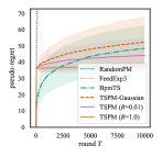
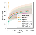
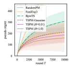
In this section, we numerically compare the performance of TSPM and TSPM-Gaussian against existing methods, which are RandomPM (the algorithm which selects action randomly), FeedExp3 (Piccolboni and Schindelhauer, 2001), and BPM-TS (Vanchinathan et al., 2014). Recently, Lattimore and Szepesvári (2019) considered the sampling-based algorithm called Mario sampling for easy games. Mario sampling coincides with TS (except for the difference between pseudo-regret and regret with known time horizon) mentioned in the last section when any pair of actions is a neighbor. As shown in Appendix G, this property is indeed satisfied for dp-easy games defined in the following. Therefore, the performance is essentially the same between TSPM with R=1R=1 and Mario sampling. To compare the performance, we consider a dynamic pricing problem, which is a typical example of PM games. We conducted experiments on the discrete setting because the experiments for PM has been mainly focused on the discrete setting.

In the dynamic pricing game, the player corresponds to a seller, and the opponent corresponds to a buyer. At each round, the seller sells an item for a specific price i(t)i(t), and the buyer comes with an evaluation price j(t)j(t) for the item, where the selling price and the evaluation price correspond to the action and outcome, respectively. The buyer buys the item if the selling price i(t)i(t) is smaller than or equal to j(t)j(t) and not otherwise. The seller can only know if the buyer bought the item (denoted as feedback 0) or did not buy the item (denoted as 11). The seller aims to minimize the cumulative “loss”, and there are two types of definitions for the loss, where each induced game falls into the easy and hard games. We call them dp-easy and dp-hard games, respectively.

In both cases, the seller incurs the constant loss c>0c>0 when the item is not bought due to the loss of opportunity to sell the item. In contrast, when the item is not bought, the loss incurred to the seller is different between these settings. The seller in the dp-easy game does not take the buyer’s evaluation price into account. In other words, the seller gains the selling price i(t)i(t) as a reward (equivalently incurs i(t)-i(t) as a loss). Therefore, the loss for the selling price i(t)i(t) and the evaluation j(t)j(t) is

i(t),j(t)=i(t)𝟙[i(t)j(t)]+c𝟙[i(t)>j(t)].\displaystyle\ell_{i(t),j(t)}=-i(t)\mathbbm{1}{\left[i(t)\leq j(t)\right]}+c\mathbbm{1}{\left[i(t)>j(t)\right]}\,.

This setting can be regarded as a generalized version of the online posted price mechanism, which was addressed in, e.g.,  Blum et al. (2004) and Cesa-Bianchi et al. (2006), and an example of strongly locally observable games.

On the other hand, the seller in dp-hard game does take the buyer’s evaluation price into account when the item is bought. In other words, the seller incurs the difference between the opponent evaluation and the selling price j(t)i(t)j(t)-i(t) as a loss because the seller could have made more profit if the seller had sold at the price j(t)j(t). Therefore, the loss incurred at time tt is

i(t),j(t)=(j(t)i(t))𝟙[i(t)j(t)]+c𝟙[i(t)>j(t)].\displaystyle\ell_{i(t),j(t)}=(j(t)-i(t))\mathbbm{1}{\left[i(t)\leq j(t)\right]}+c\mathbbm{1}{\left[i(t)>j(t)\right]}\,.

This setting is also addressed in Cesa-Bianchi et al. (2006), and belongs to the class of hard games. Note that our algorithm can also be applied to a hard game, though there is no theoretical guarantee.

Refer to caption
(a) dp-easy, N=M=3N=M=3
Refer to caption
(b) dp-easy, N=M=5N=M=5
Refer to caption
(c) dp-easy, N=M=7N=M=7
Refer to caption
(d) dp-hard, N=M=3N=M=3
Refer to caption
(e) dp-hard, N=M=5N=M=5
Refer to caption
(f) dp-hard, N=M=7N=M=7
Figure 1: Regret-round plots of algorithms. The solid lines indicate the average over 100100 independent trials. The thin fillings are the standard error.
Refer to caption
(a) dp-easy, N=M=3N=M=3
Refer to caption
(b) dp-easy, N=M=5N=M=5
Refer to caption
(c) dp-easy, N=M=7N=M=7
Figure 2: The number of rejected times by the accept-reject sampling. The solid lines indicate the average over 100100 independent trials after taking moving average with window size 100100.

Setup. In the both dp-easy and dp-hard games, we fixed N=M{3,5,7}N=M\in{\left\{3,5,7\right\}} and c=2c=2. We fixed the time horizon TT to 1000010000 and simulated 100100 times. For FeedExp3 and BPM-TS, the setup of hyperparameters follows their original papers. For TSPM, we set λ=0.001\lambda=0.001, and RR was selected from {0.01,1.0}{\left\{0.01,1.0\right\}}. Here, recall that TSPM with R=1R=1 and R=0R=0 correspond to the exact sampling and TSPM-Gaussian, respectively, and a smaller value of RR gives the higher acceptance probability in the accept-reject sampling. Therefore, using small RR makes the algorithm time-efficient, although it can worsen the performance since it over-explores the tail of the posterior distributions. To stabilize sampling from the proposal distribution in Algorithm 3, we used an initialization that takes each action n=10An=10A times. The detailed settings of the experiments with more results are given in Appendix H.

Results. Figure 1 is the empirical comparison of the proposed algorithms against the benchmark methods. This result shows that, in all cases, the TSPM with exact sampling gives the best performance. TSPM-Gaussian also outperforms BPM-TS even though both of them use Gaussian distributions as posteriors. Besides, the experimental results suggest that our algorithm performs reasonably well even for a hard game. It can be observed that the proposed methods outperform BPM-TS more significantly for a larger number of outcomes. Further discussion for this observation is given in Appendix D.

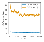
Figure 2 shows the number of rejections at each time step in the accept-reject sampling. We counted the number of times that either Line 2 in Algorithm 2 or Line 3 in Algorithm 3 was not satisfied. In the accept-reject sampling, it is desirable that the frequency of rejection does not increase as the time-step tt and does not increase rapidly with the number of outcomes. We can see that the former one is indeed satisfied. For the latter property, the frequency of rejection becomes unfortunately large when exact sampling (R=1R=1) is conducted. Still, we can substantially improve this frequency by setting RR to be a small value or zero, which still keeps regret tremendously better than that of BPM with almost the same time-efficiency as BPM-TS.

6 Conclusion and Discussion

This paper investigated Thompson sampling (TS) for stochastic partial monitoring from the algorithmic and theoretical viewpoints. We provided a new algorithm that enables exact sampling from the posterior distribution, and numerically showed that the proposed algorithm outperforms existing methods. Besides, we provided an upper bound for the problem-dependent logarithmic expected pseudo-regret for the linearized version of the partial monitoring. To our knowledge, this bound is the first logarithmic problem-dependent expected pseudo-regret bound of a TS-based algorithm for linear bandit problems and strongly locally observable partial monitoring games.

There are several remaining questions. As mentioned in Section 4, Kirschner et al. (2020) considered linear partial monitoring with the feedback structure y(t)=Si(t)p+ϵty(t)=S_{i(t)}p^{*}+\epsilon_{t}, where (ϵt)t=1T(\epsilon_{t})_{t=1}^{T} is a sequence of independent sub-Gaussian noise vector in M\mathbb{R}^{M}. This setting is the generalization of our linear setting, where (ϵt)t=1T(\epsilon_{t})_{t=1}^{T} are i.i.d. Gaussian vectors. Therefore, a natural question that arises is whether we can extend our analysis on TSPM-Gaussian to the sub-Gaussian case, although we believe it would be not straightforward as discussed in Section 4. It is also an important open problem to derive a regret bound on TSPM using the exact posterior sampling for the discrete partial monitoring. Although we conjecture that the algorithm also achieves logarithmic regret for the setting, there still remain some difficulties in the analysis. In particular, we have to handle the KL divergence in ft(p)f_{t}(p) and consider the restriction of the support of the opponent’s strategy to 𝒫M\mathcal{P}_{M}, which make the analysis much more complicated. Besides, it is worth noting that the theoretical analysis of TS for hard games has never been theoretically investigated. We believe that in general TS suffers linear regret in the minimax sense due to its greediness. However, we conjecture that TS can achieve the sub-linear regret for some specific instances of hard games in the sense of the problem-dependent regret, as empirically observed in the experiments. Finally, it is an important open problem to derive the minimax regret for anytime TS-based algorithms. This needs more detailed analysis on o(logT)\operatorname{o}(\log T) terms in the regret bound, which were dropped in our main result.

Broader Impact

Application. Partial monitoring (PM) includes various online decision-making problems such as multi-armed bandits, linear bandits, dynamic pricing, and label efficient prediction. Not only can PM handles them, the dueling bandits, combinatorial bandits, transductive bandits, and many other problems can be seen as a partial monitoring game, as discussed in Kirschner et al. (2020). Therefore, our analysis of Thompson sampling (TS) for PM games pushes the application of TS to a more wide range of online decision-making problems forward. Moreover, PM has the potential that novel online-decision making problems are newly discovered, where we have to handle the limited feedback in an online fashion.

Practical Use. The obvious advantage of using TS is that the users can easily apply the algorithm to their problems. They do not have to solve mathematical optimization problems, which are often required to solve when using non-sampling-based algorithms  (Bartók et al., 2012; Komiyama et al., 2015). For the negative side, the theoretical analysis for the regret upper bound might make the users become overconfident when the users use their algorithms. For example, they might use the TSPM algorithm to the linear PM game with heavy-tailed noise, such as sub-exponential noise, without noticing it. Nevertheless, this is not an TS-specific problem, but one that can be found in many theoretical studies, and TS is still one of the most promising policies.

Acknowledgements

The authors would like to thank the meta-reviewer and reviewers for a lot of helpful comments. The authors would like to thank Kento Nozawa and Ikko Yamane for maintaining servers for our experiments, and Kenny Song for helpful discussion on the writing. TT was supported by Toyota-Dwango AI Scholarship, and RIKEN Junior Research Associate Program for the final part of the project. JH was supported by KAKENHI 18K17998, and MS was supported by KAKENHI 17H00757.

References

  • Abbasi-Yadkori et al. (2011) Yasin Abbasi-Yadkori, Dávid Pál, and Csaba Szepesvári. Improved algorithms for linear stochastic bandits. In Advances in Neural Information Processing Systems 24, pages 2312–2320, 2011.
  • Agrawal and Goyal (2012) Shipra Agrawal and Navin Goyal. Analysis of Thompson sampling for the multi-armed bandit problem. In the 25th Annual Conference on Learning Theory, volume 23, pages 39.1–39.26, 2012.
  • Agrawal and Goyal (2013a) Shipra Agrawal and Navin Goyal. Further optimal regret bounds for Thompson sampling. In the Sixteenth International Conference on Artificial Intelligence and Statistics, volume 31, pages 99–107, 2013a.
  • Agrawal and Goyal (2013b) Shipra Agrawal and Navin Goyal. Thompson sampling for contextual bandits with linear payoffs. In the 30th International Conference on Machine Learning, pages 127–135, 2013b.
  • Altmann et al. (2014) Yoann Altmann, Steve McLaughlin, and Nicolas Dobigeon. Sampling from a multivariate gaussian distribution truncated on a simplex: A review. In 2014 IEEE Workshop on Statistical Signal Processing (SSP), pages 113–116, 2014.
  • Bartók et al. (2010) Gábor Bartók, Dávid Pál, and Csaba Szepesvári. Toward a classification of finite partial-monitoring games. In Algorithmic Learning Theory, pages 224–238, 2010.
  • Bartók et al. (2012) Gábor Bartók, Navid Zolghadr, and Csaba Szepesvári. An adaptive algorithm for finite stochastic partial monitoring. In the 29th International Conference on Machine Learning, pages 1–20, 2012.
  • Bartók et al. (2011) Gábor Bartók, Dávid Pál, and Csaba Szepesvári. Minimax regret of finite partial-monitoring games in stochastic environments. In the 24th Annual Conference on Learning Theory, volume 19, pages 133–154, 2011.
  • Blum et al. (2004) Avrim Blum, Vijay Kumar, Atri Rudra, and Felix Wu. Online learning in online auctions. Theoretical Computer Science, 324(2):137–146, 2004.
  • Casella et al. (2004) George Casella, Christian P. Robert, and Martin T. Wells. Generalized accept-reject sampling schemes, volume 45 of Lecture Notes–Monograph Series, pages 342–347. Institute of Mathematical Statistics, 2004.
  • Cesa-Bianchi et al. (2005) Nicolò Cesa-Bianchi, Gábor Lugosi, and Gilles Stoltz. Minimizing regret with label efficient prediction. IEEE Transactions on Information Theory, 51(6):2152–2162, 2005.
  • Cesa-Bianchi et al. (2006) Nicolò Cesa-Bianchi, Gábor Lugosi, and Gilles Stoltz. Regret minimization under partial monitoring. Mathematics of Operations Research, 31(3):562–580, 2006.
  • Chapelle and Li (2011) Olivier Chapelle and Lihong Li. An empirical evaluation of Thompson sampling. In Advances in Neural Information Processing Systems 24, pages 2249–2257, 2011.
  • Dani et al. (2008) Varsha Dani, Thomas P. Hayes, and Sham M. Kakade. Stochastic linear optimization under bandit feedback. In 21st Annual Conference on Learning Theory, pages 355–366, 2008.
  • Honda and Takemura (2014) Junya Honda and Akimichi Takemura. Optimality of Thompson sampling for Gaussian bandits depends on priors. In the Seventeenth International Conference on Artificial Intelligence and Statistics, volume 33, pages 375–383, 2014.
  • Jamieson et al. (2014) Kevin Jamieson, Matthew Malloy, Robert Nowak, and Sébastien Bubeck. lil’ ucb : An optimal exploration algorithm for multi-armed bandits. In The 27th Conference on Learning Theory, pages 423–439, 2014.
  • Kaufmann et al. (2012) Emilie Kaufmann, Nathaniel Korda, and Rémi Munos. Thompson sampling: An asymptotically optimal finite-time analysis. In Algorithmic Learning Theory, pages 199–213, 2012.
  • Kirschner et al. (2020) Johannes Kirschner, Tor Lattimore, and Andreas Krause. Information directed sampling for linear partial monitoring. arXiv preprint arXiv:2002.11182, 2020.
  • Kleinberg and Leighton (2003) Robert Kleinberg and Tom Leighton. The value of knowing a demand curve: Bounds on regret for online posted-price auctions. In the 44th Annual IEEE Symposium on Foundations of Computer Science, pages 594–605, 2003.
  • Komiyama et al. (2015) Junpei Komiyama, Junya Honda, and Hiroshi Nakagawa. Regret lower bound and optimal algorithm in finite stochastic partial monitoring. In Advances in Neural Information Processing Systems 28, pages 1792–1800, 2015.
  • Korda et al. (2013) Nathaniel Korda, Emilie Kaufmann, and Remi Munos. Thompson sampling for 1-dimensional exponential family bandits. In Advances in Neural Information Processing Systems 26, pages 1448–1456, 2013.
  • Lai and Robbins (1985) T. L. Lai and Herbert Robbins. Asymptotically efficient adaptive allocation rules. Advances in Applied Mathematics, 6(1):4–22, 1985.
  • Lattimore and Szepesvári (2019) Tor Lattimore and Csaba Szepesvári. An information-theoretic approach to minimax regret in partial monitoring. In the 32nd Annual Conference on Learning Theory, volume 99, pages 2111–2139, 2019.
  • Lu and Van Roy (2017) Xiuyuan Lu and Benjamin Van Roy. Ensemble sampling. In Advances in Neural Information Processing Systems 30, pages 3258–3266, 2017.
  • Phan et al. (2019) My Phan, Yasin Abbasi Yadkori, and Justin Domke. Thompson sampling and approximate inference. In Advances in Neural Information Processing Systems 32, pages 8804–8813, 2019.
  • Piccolboni and Schindelhauer (2001) Antonio Piccolboni and Christian Schindelhauer. Discrete prediction games with arbitrary feedback and loss. In COLT/EuroCOLT, pages 208–223, 2001.
  • Russo et al. (2018) Daniel J. Russo, Benjamin Van Roy, Abbas Kazerouni, Ian Osband, and Zheng Wen. A tutorial on Thompson sampling. Foundations and Trends in Machine Learning, 11(1):1–96, 2018.
  • Rustichini (1999) Aldo Rustichini. Minimizing regret: The general case. Games and Economic Behavior, 29(1):224–243, 1999.
  • Thompson (1933) William R Thompson. On the likelihood that one unknown probability exceeds another in view of the evidence of two samples. Biometrika, 25(3-4):285–294, 12 1933.
  • Vanchinathan et al. (2014) Hastagiri P Vanchinathan, Gábor Bartók, and Andreas Krause. Efficient partial monitoring with prior information. In Advances in Neural Information Processing Systems 27, pages 1691–1699, 2014.
  • Zimmert and Lattimore (2019) Julian Zimmert and Tor Lattimore. Connections between mirror descent, thompson sampling and the information ratio. In Advances in Neural Information Processing Systems 32, pages 11973–11982, 2019.
  • Zinkevich (2003) Martin Zinkevich. Online convex programming and generalized infinitesimal gradient ascent. In the Twentieth International Conference on Machine Learning, pages 928–935. AAAI Press, 2003.

Appendix A Notation

Table 1 summarizes the symbols used in this paper.

Table 1: List of symbols used in this paper.
Symbol Meaning
𝒫n\mathcal{P}_{n} (n1)(n-1)-dimensional probability simplex
\|\cdot\| Euclidian norm for vector and operator norm for matrix
p\|\cdot\|_{p} pp-norm
A\|\cdot\|_{A} norm induced by positive semidefinite matrix AA
𝒟KL(pq)\mathcal{D}_{\mathrm{KL}}\left({p}\middle\|{q}\right) KL divergence from qq to pp
Brn(p)B_{r}^{n}(p) nn-dimensional Euclidian ball of radius rr at point pNp\in\mathbb{R}^{N}
N,MN,M\in\mathbb{N} the number of actions and outcomes
Σ\Sigma set of feedback symbols
AA the number of feedback symbols
p𝒫Mp^{*}\in\mathcal{P}_{M} opponent’s strategy
TT time horizon
𝐋=(i,j)N×M\mathbf{L}=(\ell_{i,j})\in\mathbb{R}^{N\times M} loss matrix
𝐇=(hi,j)ΣN×M\mathbf{H}=(h_{i,j})\in\Sigma^{N\times M} feedback matrix
Si{0,1}A×M(i=1,,N)S_{i}\in{\left\{0,1\right\}}^{A\times M}\;(i=1,\dots,N) signal matrix
i(t)i(t) action taken at time tt
Ni(t)N_{i}(t) the number of times the action ii is taken before time t[T]t\in[T]
j(t)j(t) outcome taken by opponent at time tt
y(t)y(t) feedback observed at time tt
Ft(p)F_{t}(p) unnormalized posterior distribution in (1)
ft(p)f_{t}(p) probability density function corresponding to Ft(p)F_{t}(p)
Gt(p)G_{t}(p) unnormalized proposal distribution for Ft(p)F_{t}(p) in (2)
gt(p)g_{t}(p) probability density function corresponding to Gt(p)G_{t}(p)
qi(t)𝒫Mq_{i}^{(t)}\in\mathcal{P}_{M} empirical feedback distribution of action ii by time tt
qi,n𝒫Mq_{i,n}\in\mathcal{P}_{M} empirical feedback distribution of action ii after the action is taken nn times
𝒞i𝒫M\mathcal{C}_{i}\subset\mathcal{P}_{M} cell of action ii

Appendix B Posterior Distribution and Proposal Distribution in Section 3

In this appendix, we discuss representation of the posterior distribution and its relation with the proposal distribution.

Proposition 4.

Ft(p)F_{t}(p) in (1) is proportional to the posterior distribution of the opponent’s strategy, and Ft(p)Gt(p)F_{t}(p)\leq G_{t}(p) for all p𝒫Mp\in\mathcal{P}_{M}.

Proof.

The posterior distribution of the opponent’s strategy parameter π(p|{i(s),y(s)}s=1t)\pi{\left(p\mathrel{}\middle|\mathrel{}{\left\{i(s),y(s)\right\}}_{s=1}^{t}\right)} is rewritten as

π(p|{i(s),y(s)}s=1t)\displaystyle\pi{\left(p\mathrel{}\middle|\mathrel{}{\left\{i(s),y(s)\right\}}_{s=1}^{t}\right)} π(p,{i(s),y(s)}s=1t)\displaystyle\propto\pi{\left(p,{\left\{i(s),y(s)\right\}}_{s=1}^{t}\right)}
π(p)s=1t{y(s)|i(s),p}\displaystyle\propto\pi{\left(p\right)}\prod_{s=1}^{t}\mathbb{P}{\left\{y(s)\mathrel{}\middle|\mathrel{}i(s),p\right\}}
=π(p)i=1Ny=1A(Si,yp)niy\displaystyle=\pi{\left(p\right)}\prod_{i=1}^{N}\prod_{y=1}^{A}(S_{i,y}p)^{n_{iy}}
π(p)i=1Nexp{ni𝒟KL(qi(t)Sip)},\displaystyle\propto\pi{\left(p\right)}\prod_{i=1}^{N}\exp\Big{\{}-n_{i}\mathcal{D}_{\mathrm{KL}}\left({q_{i}^{(t)}}\middle\|{S_{i}p}\right)\Big{\}}\,, (5)

where Si,yS_{i,y} is the ii-th row of the signal matrix SiS_{i}, and note that qi(t)q_{i}^{(t)} is the empirical feedback distribution of action ii at time tt, that is, qi(t)=[ni1/ni,,niA/ni]𝒫Aq_{i}^{(t)}=[n_{i1}/n_{i},\ldots,n_{iA}/n_{i}]^{\top}\in\mathcal{P}_{A} for niy=s=1t𝟙[i(s)=i,y(s)=y]n_{iy}=\sum_{s=1}^{t}\mathbbm{1}{\left[i(s)=i,y(s)=y\right]} and ni=y=1Aniyn_{i}=\sum_{y=1}^{A}n_{iy}.

Next, we show that Ft(p)Gt(p)F_{t}(p)\leq G_{t}(p) holds for all p𝒫Mp\in\mathcal{P}_{M}. Using the Pinsker’s inequality, the unnormalized posterior distribution Ft(p)F_{t}(p) can be bounded from above as

Ft(p)\displaystyle F_{t}(p) =π(p)i=1Nexp{ni𝒟KL(qi(t)Sip)}\displaystyle=\pi{\left(p\right)}\prod_{i=1}^{N}\exp\Big{\{}-n_{i}\mathcal{D}_{\mathrm{KL}}\left({q_{i}^{(t)}}\middle\|{S_{i}p}\right)\Big{\}}
π(p)i=1Nexp{12niqi(t)Sip12}(by Pinsker’s ineq.)\displaystyle\leq\pi{\left(p\right)}\prod_{i=1}^{N}\exp\Big{\{}-\frac{1}{2}n_{i}\|q_{i}^{(t)}-S_{i}p\|_{1}^{2}\Big{\}}\quad\left(\text{by {Pinsker's ineq.}}\right)
=π(p)exp{12i=1Nniqi(t)Sip12}\displaystyle=\pi{\left(p\right)}\exp\Big{\{}-\frac{1}{2}\sum_{i=1}^{N}n_{i}\|q_{i}^{(t)}-S_{i}p\|_{1}^{2}\Big{\}}
π(p)exp{12i=1Nniqi(t)Sip2}(by qi(t)Sip1qi(t)Sip)\displaystyle\leq\pi{\left(p\right)}\exp\Big{\{}-\frac{1}{2}\sum_{i=1}^{N}n_{i}\|q_{i}^{(t)}-S_{i}p\|^{2}\Big{\}}\quad\left(\text{by }{\|q_{i}^{(t)}-S_{i}p\|_{1}\geq\|q_{i}^{(t)}-S_{i}p\|}\right)
=Gt(p).\displaystyle=G_{t}(p)\,. (6)

Remark.

The unnormalized density Gt(p)G_{t}(p) is indeed Gaussian. Recalling that BtB_{t} and btb_{t} are defined in (3) as

Bt=i=1NniSiSi=s=1tSi(s)Si(s)=Bt1+Si(t)Si(t),bt=i=1NniSiqi(t)=bt1+Si(t)ey(t),\displaystyle B_{t}=\sum_{i=1}^{N}n_{i}S_{i}^{\top}S_{i}=\sum_{s=1}^{t}S_{i(s)}^{\top}S_{i(s)}=B_{t-1}+S_{i(t)}^{\top}S_{i(t)},\quad b_{t}=\sum_{i=1}^{N}n_{i}S_{i}^{\top}q_{i}^{(t)}=b_{t-1}+S_{i(t)}^{\top}e_{y(t)}\,, (7)

we have

i=1Nniqi(t)Sip2\displaystyle\sum_{i=1}^{N}n_{i}\|q_{i}^{(t)}-S_{i}p\|^{2} =i=1Nni(qi(t)Sip)(qi(t)Sip)\displaystyle=\sum_{i=1}^{N}n_{i}(q_{i}^{(t)}-S_{i}p)^{\top}(q_{i}^{(t)}-S_{i}p)
=p(i=1NniSiSi)Btp,2(i=1NniSiqi(t))btp+i=1Nniqi(t)2ct\displaystyle=p^{\top}\underbrace{\Big{(}\sum_{i=1}^{N}n_{i}S_{i}^{\top}S_{i}\Big{)}}_{B_{t}}p,-2\underbrace{\Big{(}\sum_{i=1}^{N}n_{i}S_{i}^{\top}q_{i}^{(t)}\Big{)}^{\top}}_{b_{t}}p+\underbrace{\sum_{i=1}^{N}n_{i}\|q_{i}^{(t)}\|^{2}}_{c_{t}}
=pBtp2btp+ct\displaystyle=p^{\top}B_{t}p-2b_{t}^{\top}p+c_{t}
=(pBt1bt)Bt(pBt1bt)+ctbtBt1bt.\displaystyle=(p-B_{t}^{-1}b_{t})^{\top}B_{t}(p-B_{t}^{-1}b_{t})+c_{t}-b_{t}^{\top}B_{t}^{-1}b_{t}\,. (8)

Therefore, we have

exp{12i=1Nniqi(t)Sip2}\displaystyle\exp\Big{\{}-\frac{1}{2}\sum_{i=1}^{N}n_{i}\|q_{i}^{(t)}-S_{i}p\|^{2}\Big{\}} exp{12(pBt1bt)Bt(pBt1bt)}.\displaystyle\propto\exp\Big{\{}-\frac{1}{2}(p-B_{t}^{-1}b_{t})^{\top}B_{t}(p-B_{t}^{-1}b_{t})\Big{\}}\,. (9)

Appendix C Proof of Proposition 2

We will see that the the procedure sampling p~t\tilde{p}_{t} from gt(p)g_{t}(p) and Algorithm 3 are equivalent. First, we derive the Gaussian density of gt(p)g_{t}(p) projected onto {pM:i=1Mpi=1}\{p\in\mathbb{R}^{M}:\sum_{i=1}^{M}p_{i}=1\}.

For simplicity, we omit the subscript tt and write, e.g., BB instead of BtB_{t}. We define p=[p(α),pM]M1×p=[{p^{(\alpha)}}^{\top},p_{M}]^{\top}\in\mathbb{R}^{M-1}\times\mathbb{R}. Let h=B1bh=B^{-1}b, and define h=[h(α),hM]M1×h=[{h^{(\alpha)}}^{\top},h_{M}]^{\top}\in\mathbb{R}^{M-1}\times\mathbb{R}. Let B=[Cddf]B=\begin{bmatrix}C&d\\ d^{\top}&f\\ \end{bmatrix}, where CM1×M1,dM1C\in\mathbb{R}^{{M-1}\times{M-1}},d\in\mathbb{R}^{M-1}, and ff\in\mathbb{R}. Also, let b=[b(α),b(M)]M1×b=[{b^{(\alpha)}}^{\top},b^{(M)}]^{\top}\in\mathbb{R}^{M-1}\times\mathbb{R}.

Using the decomposition

(pB1b)B(pB1b)\displaystyle(p-B^{-1}b)^{\top}B(p-B^{-1}b) =pBp(a)2hBp(b)+hBh,\displaystyle=\underbrace{p^{\top}Bp}_{\text{(a)}}-2\underbrace{h^{\top}Bp}_{\text{(b)}}+h^{\top}Bh\,, (10)

we rewrite each term by restricting the domain of pp so that it satisfies the condition i=1Mpi=1\sum_{i=1}^{M}p_{i}=1. Now the first term (a) is rewritten as

(a) =p(α)Cp(α)+2p(α)dpM+fpM2\displaystyle={p^{(\alpha)}}^{\top}C{p^{(\alpha)}}+2{p^{(\alpha)}}^{\top}dp_{M}+fp_{M}^{2}
=p(α)Cp(α)+2p(α)d(1i=1M1pi)(a1)+f(1i=1M1pi)2(a2).\displaystyle={p^{(\alpha)}}^{\top}C{p^{(\alpha)}}+2\underbrace{{p^{(\alpha)}}^{\top}d\Big{(}1-\sum_{i=1}^{M-1}p_{i}\Big{)}}_{\text{(a1)}}+f\underbrace{\Big{(}1-\sum_{i=1}^{M-1}p_{i}\Big{)}^{2}}_{\text{(a2)}}\,. (11)

The term (a1) is rewritten as

(a1) =p(α)dp(α)di=1M1pi\displaystyle={p^{(\alpha)}}^{\top}d-{p^{(\alpha)}}^{\top}d\sum_{i=1}^{M-1}p_{i}
=p(α)dp(α)d𝟏M1p(α)\displaystyle={p^{(\alpha)}}^{\top}d-{p^{(\alpha)}}^{\top}d\mathbf{1}_{M-1}^{\top}{p^{(\alpha)}}
=p(α)dp(α)Dp(α)(D=12(d𝟏M1+𝟏M1d)),\displaystyle={p^{(\alpha)}}^{\top}d-{p^{(\alpha)}}^{\top}D{p^{(\alpha)}}\quad\left(D=\frac{1}{2}\left(d\mathbf{1}_{M-1}^{\top}+\mathbf{1}_{M-1}d^{\top}\right)\right)\,, (12)

and the term (a2) is rewritten as

(a2) =(1i=1M1pi)2\displaystyle=\Big{(}1-\sum_{i=1}^{M-1}p_{i}\Big{)}^{2}
=12i=1M1pi+(i=1M1pi)2\displaystyle=1-2\sum_{i=1}^{M-1}p_{i}+\Big{(}\sum_{i=1}^{M-1}p_{i}\Big{)}^{2}
=12𝟏M1p(α)+p(α)𝟏M1𝟏M1p(α).\displaystyle=1-2\mathbf{1}_{M-1}^{\top}{p^{(\alpha)}}+{p^{(\alpha)}}^{\top}\mathbf{1}_{M-1}\mathbf{1}_{M-1}^{\top}{p^{(\alpha)}}\,. (13)

Therefore,

(a) =p(α)(C2D+f𝟏M1𝟏M1)B~p(α)2(f𝟏M1d)p(α)+f.\displaystyle={p^{(\alpha)}}^{\top}\underbrace{(C-2D+f\mathbf{1}_{M-1}\mathbf{1}_{M-1}^{\top})}_{\tilde{B}}{p^{(\alpha)}}-2(f\mathbf{1}_{M-1}-d)^{\top}{p^{(\alpha)}}+f\,. (14)

With regard to the term (b), we have

(b) =bp\displaystyle=b^{\top}p
=b(α)p(α)+b(M)pM\displaystyle={b^{(\alpha)}}^{\top}{p^{(\alpha)}}^{\top}+b^{(M)}p_{M}
=(b(α)b(M)𝟏M1)p(α)+b(M).\displaystyle=({b^{(\alpha)}}-b^{(M)}\mathbf{1}_{M-1})^{\top}{p^{(\alpha)}}+b^{(M)}\,. (15)

Therefore,

(pB1b)B(pB1b)\displaystyle(p-B^{-1}b)^{\top}B(p-B^{-1}b)
=p(α)B~p(α)2(f𝟏M1d+b(α)b(M)𝟏M1b~)p(α)+f2b(M)+hBh\displaystyle={p^{(\alpha)}}^{\top}\tilde{B}{p^{(\alpha)}}-2(\underbrace{f\mathbf{1}_{M-1}-d+{b^{(\alpha)}}-b^{(M)}\mathbf{1}_{M-1}}_{\tilde{b}})^{\top}{p^{(\alpha)}}+f-2b^{(M)}+h^{\top}Bh
=(p(α)B~1b~)B~(p(α)B~1b~)+f2b(M)b~B~1b~+bB1b(by hBh=bB1b).\displaystyle=({p^{(\alpha)}}-\tilde{B}^{-1}\tilde{b})^{\top}\tilde{B}({p^{(\alpha)}}-\tilde{B}^{-1}\tilde{b})+f-2b^{(M)}-\tilde{b}^{\top}\tilde{B}^{-1}\tilde{b}+b^{\top}B^{-1}b\quad\quad\left(\text{by }{h^{\top}Bh=b^{\top}B^{-1}b}\right)\,. (16)

From the above argument, the density 𝒩(B~1b,B~1)\mathcal{N}(\tilde{B}^{-1}b,\,\tilde{B}^{-1}) is the Gaussian distribution of gt(p)g_{t}(p) on {pM:i=1Mpi=1}\{p\in\mathbb{R}^{M}:\sum_{i=1}^{M}p_{i}=1\}. Therefore, the p=[p(α), 1i=1M1(p(α))i]p=[{p^{(\alpha)}}^{\top},\,1-\sum_{i=1}^{M-1}({p^{(\alpha)}})_{i}]^{\top} for p(α)𝒩(B~1b,B~1){p^{(\alpha)}}\sim\mathcal{N}(\tilde{B}^{-1}b,\,\tilde{B}^{-1}) is supported over {pM:i=1Mpi=1}\{p\in\mathbb{R}^{M}:\sum_{i=1}^{M}p_{i}=1\}.

If the sample p(α){p^{(\alpha)}} from 𝒩(B~1b,B~1)\mathcal{N}(\tilde{B}^{-1}b,\,\tilde{B}^{-1}) is in 𝒫M1\mathcal{P}_{M-1}, then we can obtain the last element p(M)p^{(M)} by p(M)=1i=1M1(p(α))ip^{(M)}=1-\sum_{i=1}^{M-1}({p^{(\alpha)}})_{i}. Otherwise, the probability that p(α){p^{(\alpha)}} is the first M1M-1 elements of the sample from gt(p)g_{t}(p) is zero, and hence, [p(α),p(M)][{p^{(\alpha)}}^{\top},p^{(M)}]^{\top} cannot be a sample from gt(p)g_{t}(p). Therefore, sampling p~t\tilde{p}_{t} from gt(p)g_{t}(p) and Algorithm 3 are equivalent.

Appendix D Relation between TSPM-Gaussian and BPM-TS

In this appendix, we discuss the relation between TSPM-Gaussian and BPM-TS (Vanchinathan et al., 2014).

Underlying Feedback Structure. Here, we discuss the underlying feedback structure behind TSPM-Gaussian and BPM-TS.

We first consider the underlying feedback structure behind BPM-TS. In the following, we see that the feedback structure

y(t)=Si(t)p+Si(t)ϵ,ϵ𝒩(0,IM)\displaystyle y(t)=S_{i(t)}p+S_{i(t)}\epsilon\,,\;\epsilon\sim\mathcal{N}(0,I_{M}) (17)

induces the posterior distribution in BPM-TS. Under this feedback structure, we have y(t)𝒩(Si(t)p,Si(t)Si(t))y(t)\sim\mathcal{N}(S_{i(t)}p,S_{i(t)}S_{i(t)}^{\top}).

When we take the prior distribution π(p)\pi{\left(p\right)} as 𝒩(0,σ02IM)\mathcal{N}(0,\sigma_{0}^{2}I_{M}), the posterior distribution for the opponent’s strategy parameter can be written as

π(p|{i(s),y(s)}s=1t)\displaystyle\pi{\left(p\mathrel{}\middle|\mathrel{}{\left\{i(s),y(s)\right\}}_{s=1}^{t}\right)}
π(p)s=1tπ(y(s)|i(s),p)\displaystyle\propto\pi{\left(p\right)}\prod_{s=1}^{t}\pi{\left(y(s)\mathrel{}\middle|\mathrel{}i(s),\,p\right)}
=π(p)s=1ty𝒩(Si(s)p,Si(s)Si(s)){y=y(s)}\displaystyle=\pi{\left(p\right)}\prod_{s=1}^{t}\mathbb{P}_{y\sim\mathcal{N}(S_{i(s)}p,S_{i(s)}S_{i(s)}^{\top})}\left\{y=y(s)\right\}
=exp(pp2σ02)s=1texp(12(y(s)Si(s)p)(Si(s)Si(s))1(y(s)Si(s)p))\displaystyle=\exp\Big{(}-\frac{p^{\top}p}{2\sigma_{0}^{2}}\Big{)}\prod_{s=1}^{t}\exp\Big{(}-\frac{1}{2}(y(s)-S_{i(s)}p)^{\top}(S_{i(s)}S_{i(s)}^{\top})^{-1}(y(s)-S_{i(s)}p)\Big{)}
=exp{12(p(1σ02IM+s=1tSi(s)(Si(s)Si(s))1Si(s))p)\displaystyle=\exp\Big{\{}-\frac{1}{2}\Big{(}p^{\top}\Big{(}\frac{1}{\sigma_{0}^{2}}I_{M}+\sum_{s=1}^{t}S_{i(s)}^{\top}(S_{i(s)}S_{i(s)}^{\top})^{-1}S_{i(s)}\Big{)}p\Big{)}
2(s=1ty(s)(Si(s)Si(s))1Si(s)p)+(a term independent of p)}\displaystyle\qquad\qquad-2\Big{(}\sum_{s=1}^{t}y(s)^{\top}(S_{i(s)}S_{i(s)}^{\top})^{-1}S_{i(s)}p\Big{)}+\text{(a term independent of $p$)}\Big{\}}
exp{12(pBtBPMp2btBPMp)}\displaystyle\propto\exp\Big{\{}-\frac{1}{2}(p^{\top}{B_{t}^{\mathrm{BPM}}}p-2{b_{t}^{\mathrm{BPM}}}^{\top}p)\Big{\}}
exp{12(pBtBPM1btBPM)BtBPM(pBtBPM1btBPM)},\displaystyle\propto\exp\Big{\{}-\frac{1}{2}(p-{{B_{t}^{\mathrm{BPM}}}}^{-1}{b_{t}^{\mathrm{BPM}}})^{\top}{B_{t}^{\mathrm{BPM}}}(p-{B_{t}^{\mathrm{BPM}}}^{-1}{b_{t}^{\mathrm{BPM}}})\Big{\}}\,, (18)

where

BtBPM\displaystyle{B_{t}^{\mathrm{BPM}}} =1σ02IM+s=1tSi(s)(Si(s)Si(s))1Si(s)=Bt1BPM+Si(t)(Si(t)Si(t))1Si(t),\displaystyle=\frac{1}{\sigma_{0}^{2}}I_{M}+\sum_{s=1}^{t}S_{i(s)}^{\top}(S_{i(s)}S_{i(s)}^{\top})^{-1}S_{i(s)}=B_{t-1}^{\mathrm{BPM}}+S_{i(t)}^{\top}(S_{i(t)}S_{i(t)}^{\top})^{-1}S_{i(t)}\,, (19)
btBPM\displaystyle{b_{t}^{\mathrm{BPM}}} =s=1tSi(s)(Si(s)Si(s))1y(s)=bt1BPM+Si(t)(Si(t)Si(t))1y(t).\displaystyle=\sum_{s=1}^{t}S_{i(s)}^{\top}(S_{i(s)}S_{i(s)}^{\top})^{-1}y(s)=b_{t-1}^{\mathrm{BPM}}+S_{i(t)}^{\top}(S_{i(t)}S_{i(t)}^{\top})^{-1}y(t)\,. (20)

Therefore, the posterior distribution π(p{i(s),y(s)}s=1t)\pi{\left(p\mid{\left\{i(s),y(s)\right\}}_{s=1}^{t}\right)} is

1(2π)M|BtBPM1|exp{12(pBtBPM1btBPM)BtBPM(pBtBPM1btBPM)}.\displaystyle\frac{1}{\sqrt{(2\pi)^{M}|{B_{t}^{\mathrm{BPM}}}^{-1}|}}\exp\Big{\{}-\frac{1}{2}(p-{B_{t}^{\mathrm{BPM}}}^{-1}{b_{t}^{\mathrm{BPM}}})^{\top}{B_{t}^{\mathrm{BPM}}}(p-{B_{t}^{\mathrm{BPM}}}^{-1}{b_{t}^{\mathrm{BPM}}})\Big{\}}\,. (21)

and this distribution indeed corresponds to the posterior distribution in BPM-TS (Vanchinathan et al., 2014) with BtBPM=Σt1{B_{t}^{\mathrm{BPM}}}=\Sigma_{t}^{-1}.

Using the same argument, we can confirm that the feedback structure

yt=Sip+ϵ,ϵ𝒩(0,IM).\displaystyle y_{t}=S_{i}p+\epsilon\,,\;\epsilon\sim\mathcal{N}(0,I_{M})\,. (22)

induces

g¯t(p)1(2π)M|Bt1|exp(12pBt1btBt2),\displaystyle\bar{g}_{t}(p)\coloneqq\frac{1}{\sqrt{(2\pi)^{M}|B_{t}^{-1}|}}\exp\Big{(}-\frac{1}{2}\left\|p-B_{t}^{-1}b_{t}\right\|_{B_{t}}^{2}\Big{)}\,, (23)

which corresponds to the posterior distribution for TSPM in linear partial monitoring.

Covariances in TSPM-Gaussian and BPM-TS. In the linear partial monitoring, TSPM assumes noise with covariance IMI_{M}, which is compatible with the fact that the discrete setting can be regarded as linear PM with IMI_{M}-sub-Gaussian noise. On the other hand, BPM-TS assumes covariance SiSiS_{i}S_{i}^{\top}, and in general IMSiSiI_{M}\preceq S_{i}S_{i}^{\top} holds. Therefore, BPM-TS assumes unnecessarily larger covariance, which makes learning slow down.

Appendix E Preliminaries for Regret Analysis

In this appendix, we give some technical lemmas, which are used for the derivation of the regret bound in Appendix F. Here, we write XYX\succeq Y to denote XY0X-Y\succeq 0. For a,ba,b\in\mathbb{R}, let aba\wedge b be aa if aba\leq b otherwise bb, and aba\vee b be bb if aba\leq b otherwise aa. We use h(a)XχM2{Xa}h(a)\coloneqq\mathbb{P}_{X\sim\chi^{2}_{M}}\left\{X\geq a\right\} to evaluate the behavior of the posterior samples, where χM2\chi^{2}_{M} is the chi-squared distribution with MM degree of freedom.

E.1 Basic Lemmas

Fact 5 (Moment generating function of squared-Gaussian distribution).

Let XX be the random variable following the standard normal distribution. Then, the moment generating function of X2X^{2} is 𝔼[exp(ξX2)]=(12ξ)1/2\operatornamewithlimits{\mathbb{E}}{\left[\exp(\xi X^{2})\right]}=(1-2\xi)^{-1/2} for ξ<1/2\xi<1/2.

Lemma 6 (Chernoff bound for chi-squared random variable).

Let XX be the random variable following the chi-squared distribution with kk degree of freedom. Then, for any a0a\geq 0 and 0ξ<1/20\leq\xi<1/2,

{Xa}eξa(12ξ)k2.\displaystyle\mathbb{P}{\left\{X\geq a\right\}}\leq\mathrm{e}^{-\xi a}(1-2\xi)^{-\frac{k}{2}}. (24)
Proof.

By Markov’s inequality, the LHS can be bounded as

{Xa}\displaystyle\mathbb{P}{\left\{X\geq a\right\}} ={i=1kXi2a}(X1,,Xki.i.d.𝒩(0,1))\displaystyle=\mathbb{P}{\left\{\sum_{i=1}^{k}X_{i}^{2}\geq a\right\}}\;(X_{1},\ldots,X_{k}\stackrel{{\scriptstyle\mathrm{i.i.d.}}}{{\sim}}\mathcal{N}(0,1))
={exp(ξi=1kXi2)exp(ξa)}\displaystyle=\mathbb{P}{\left\{\exp\Big{(}\xi\sum_{i=1}^{k}X_{i}^{2}\Big{)}\geq\exp(\xi a)\right\}}
eξa(𝔼[eξX12])k(by Markov’s ineq.)\displaystyle\leq\mathrm{e}^{-\xi a}\Big{(}\operatornamewithlimits{\mathbb{E}}{\left[\mathrm{e}^{\xi X_{1}^{2}}\right]}\Big{)}^{k}\quad\left(\text{by {Markov's ineq.}}\right)
=eξa(12ξ)k2(by Fact 5),\displaystyle=\mathrm{e}^{-\xi a}(1-2\xi)^{-\frac{k}{2}}\quad\left(\text{by {Fact~{}\ref{fact:mgf_sqGauss}}}\right)\,, (25)

which completes the proof. ∎

E.2 Property of Strong Local Observability

Recall that Δi=(LiL1)p>0\Delta_{i}=(L_{i}-L_{1})^{\top}p^{*}>0 for i[N]i\in[N], which is the difference of the expected loss of actions ii and 11. For this define

ϵ(12Amini1Δiz1,i)(minp𝒞1c43pp),\displaystyle\epsilon\coloneqq\left(\frac{1}{2\sqrt{A}}\min_{i\neq 1}\frac{\Delta_{i}}{\|z_{1,i}\|}\right)\wedge\left(\min_{p\in\mathcal{C}_{1}^{c}}\frac{4}{3}\|p-p^{*}\|\right)\,, (26)

which is used throughout the proof of this appendix and Appendix F. The following lemma provides the key property of the strong local observability condition.

Lemma 7.

For any partial monitoring game with strong local observability and pMp\in\mathbb{R}^{M}, any of the conditions 1–3 in the following is not satisfied:

  1. 1.

    L1p>LkpL_{1}^{\top}p>L_{k}^{\top}p   (Worse action kk looks better under pp.)

  2. 2.

    S1pS1pϵ\|S_{1}p-S_{1}p^{*}\|\leq\epsilon

  3. 3.

    SkpSkpϵ\|S_{k}p-S_{k}p^{*}\|\leq\epsilon  .

Proof.

We prove by contradiction. Assume that there exists pMp\in\mathbb{R}^{M} such that conditions 1–3 are simultaneously satisfied.

Now, by the conditions 2 and 3, we have

|S1pS1p|ϵ𝟏A,|SkpSkp|ϵ𝟏A.\displaystyle\begin{split}|S_{1}p-S_{1}p^{*}|&\preceq\epsilon\mathbf{1}_{A}\,,\\ |S_{k}p-S_{k}p^{*}|&\preceq\epsilon\mathbf{1}_{A}\,.\end{split} (27)

Here, |||\cdot| is the element-wise absolute value, and \preceq means that the inequality \leq holds for each element. Therefore,

|(S1Sk)(pp)|ϵ𝟏2A.\displaystyle\left|\left(\begin{array}[]{c}S_{1}\\ S_{k}\end{array}\right)(p-p^{*})\right|\preceq\epsilon\mathbf{1}_{2A}\,. (30)

On the other hand, by the strong local observability condition, for any k1k\neq 1, there exists z1,k02Az_{1,k}\neq 0\in\mathbb{R}^{2A} such that

(L1Lk)=z1,k(S1Sk).\displaystyle(L_{1}-L_{k})^{\top}=z_{1,k}^{\top}\left(\begin{array}[]{c}S_{1}\\ S_{k}\end{array}\right)\,. (33)

Now, we have

z1,k(S1Sk)(pp)\displaystyle z_{1,k}^{\top}\left(\begin{array}[]{c}S_{1}\\ S_{k}\end{array}\right)(p-p^{*}) (36)
z1,k(S1Sk)(pp)(by Cauchy-Schwarz ineq.)\displaystyle\leq\|z_{1,k}\|\left\|\left(\begin{array}[]{c}S_{1}\\ S_{k}\end{array}\right)(p-p^{*})\right\|\quad\left(\text{by {Cauchy-Schwarz ineq.}}\right) (39)
2Aϵz1,k(by Eq. (30)),\displaystyle\leq\sqrt{2A}\epsilon\|z_{1,k}\|\quad\left(\text{by {Eq.~{}\eqref{eq:element_wise_cond}}}\right)\,, (40)

and

z1,k(S1Sk)(pp)\displaystyle z_{1,k}^{\top}\left(\begin{array}[]{c}S_{1}\\ S_{k}\end{array}\right)(p-p^{*}) (43)
=(L1Lk)(pp)(by Eq. (33))\displaystyle=(L_{1}-L_{k})^{\top}(p-p^{*})\quad\left(\text{by {Eq.~{}\eqref{eq:loc}}}\right)
=(L1Lk)p+(LkL1)p\displaystyle=(L_{1}-L_{k})^{\top}p+(L_{k}-L_{1})^{\top}p^{*}
Δk(by Condition 1 & def. of Δk).\displaystyle\geq\Delta_{k}\quad\left(\text{by {Condition 1 \& def. of $\Delta_{k}$}}\right)\,. (44)

Therefore, from (40) and (44), we have

Δk2Aϵz1,k.\displaystyle\Delta_{k}\leq\sqrt{2A}\epsilon\|z_{1,k}\|\,. (45)

This inequality does not hold for all k1k\neq 1 for the predefined value of ϵ\epsilon, since we have

ϵ12Amink1Δkz1,k.\displaystyle\epsilon\leq\frac{1}{2\sqrt{A}}\min_{k\neq 1}\frac{\Delta_{k}}{\|z_{1,k}\|}\,. (46)

Therefore, the proof is completed by contradiction. ∎

Remark.

The similar result holds when the optimal action 11 is replaced with action jkj\neq k such that Δj,k(LjLk)p>0\Delta_{j,k}\coloneqq(L_{j}-L_{k})^{\top}p^{*}>0 by taking ϵ\epsilon satisfying

ϵ12Aminjk:Δj,k>0Δj,kzj,k.\displaystyle\epsilon\leq\frac{1}{2\sqrt{A}}\min_{j\neq k:\Delta_{j,k}>0}\frac{\Delta_{j,k}}{\|z_{j,k}\|}\,. (47)

From Lemma 7, we have the following corollary.

Corollary 8.

For any pMp\in\mathbb{R}^{M} satisfying p𝒞ip\in\mathcal{C}_{i} and S1pS1pϵ\|S_{1}p-S_{1}p^{*}\|\leq\epsilon, we have

SipSip>ϵ.\displaystyle\|S_{i}p-S_{i}p^{*}\|>\epsilon\,. (48)
Proof.

Note that p𝒞ip\in\mathcal{C}_{i} is equivalent to (L1Li)p>0(L_{1}-L_{i})^{\top}p^{*}>0 for any i1i\neq 1. Therefore, the result directly follows from Lemma 7. ∎

The next lemma is the property of Mahalanobis distance corresponding to g¯t(p)\bar{g}_{t}(p).

Lemma 9.

Define 𝒯i{pM:SipSip>ϵ}\mathcal{T}_{i}\coloneqq\{p\in\mathbb{R}^{M}:\|S_{i}p-S_{i}p^{*}\|>\epsilon\}. Assume that Ni(t)niN_{i}(t)\geq n_{i}, Sip^tSipϵ/4\|S_{i}\hat{p}_{t}-S_{i}p^{*}\|\leq\epsilon/4. Then, for any 0ξ<1/20\leq\xi<1/2

h(infp𝒯iBt1/2(pp^t)2)exp(916ξϵ2ni)(12ξ)M/2.\displaystyle h\bigg{(}\inf_{p\in\mathcal{T}_{i}}\|B_{t}^{1/2}(p-\hat{p}_{t})\|^{2}\bigg{)}\leq\exp\Big{(}-\frac{9}{16}\xi\epsilon^{2}n_{i}\Big{)}(1-2\xi)^{-M/2}\,. (49)
Proof.

To bound the LHS of the above inequality, we bound Bt1/2(pp^t)2\|B_{t}^{1/2}(p-\hat{p}_{t})\|^{2} from below for p𝒯ip\in\mathcal{T}_{i}. Using the triangle inequality and the assumptions, we have

Si(pp^t)\displaystyle\|S_{i}(p-\hat{p}_{t})\| SipSipSip^tSip\displaystyle\geq\|S_{i}p-S_{i}p^{*}\|-\|S_{i}\hat{p}_{t}-S_{i}p^{*}\|
>ϵϵ/4>0.\displaystyle>\epsilon-\epsilon/4>0\,. (50)

Therefore, we have

Bt1/2(pp^t)2\displaystyle\|B_{t}^{1/2}(p-\hat{p}_{t})\|^{2} k[N]Nk(t)Sk(pp^t)2(by def. of Bt)\displaystyle\geq\sum_{k\in[N]}N_{k}(t)\|S_{k}(p-\hat{p}_{t})\|^{2}\quad\left(\text{by {def. of $B_{t}$}}\right)
niSi(pp^t)2(Ni(t)ni)\displaystyle\geq n_{i}\|S_{i}(p-\hat{p}_{t})\|^{2}\quad\left({N_{i}(t)\geq n_{i}}\right)
>916ϵ2ni(by Eq. (50)).\displaystyle>\frac{9}{16}\epsilon^{2}n_{i}\quad\left(\text{by {Eq.~{}\eqref{eq:diff_p_phat}}}\right)\,. (51)

By the Chernoff bound for a chi-squared random variable in Lemma 6, we now have

h(a)eξa(12ξ)M/2,\displaystyle h(a)\leq\mathrm{e}^{-\xi a}(1-2\xi)^{-M/2}\,, (52)

for any a0a\geq 0 and 0ξ<1/20\leq\xi<1/2. Hence, using the fact that Bt1/2(pp^t)2\|B_{t}^{1/2}(p-\hat{p}_{t})\|^{2} follows the chi-squared distribution with MM degree of freedom, we have

h(infp𝒯iBt1/2(pp^t)2)\displaystyle h\bigg{(}\inf_{p\in\mathcal{T}_{i}}\|B_{t}^{1/2}(p-\hat{p}_{t})\|^{2}\bigg{)} h(916ϵ2ni)\displaystyle\leq h\Big{(}\frac{9}{16}\epsilon^{2}n_{i}\Big{)}
exp(916ξϵ2ni)(12ξ)M/2,\displaystyle\leq\exp\Big{(}-\frac{9}{16}\xi\epsilon^{2}n_{i}\Big{)}(1-2\xi)^{-M/2}\,, (53)

which completes the proof. ∎

E.3 Statistics of Uninterested Actions

For any kik\neq i and nk[T]n_{k}\in[T], define

Znk\displaystyle Z_{n_{k}} nkqk,nkSkp2,\displaystyle\coloneqq n_{k}\|q_{k,n_{k}}-S_{k}p^{*}\|^{2}\,, (54)
Z\i\displaystyle Z_{\backslash i} kimaxnk[T]Znk.\displaystyle\coloneqq\sum_{k\neq i}\max_{n_{k}\in[T]}Z_{n_{k}}\,. (55)

In this section, we bound 𝔼[Z\i]\operatornamewithlimits{\mathbb{E}}{\left[Z_{\backslash i}\right]} from above. Note that Z\iZ_{\backslash i} is independent of the randomness of Thompson sampling.

Lemma 10 (Upper bound for the expectation of Z\iZ_{\backslash i}).
𝔼[Z\i]4N(logT+A2log2+1).\displaystyle\operatornamewithlimits{\mathbb{E}}{\left[Z_{\backslash i}\right]}\leq 4N\Big{(}\log T+\frac{A}{2}\log 2+1\Big{)}\,. (56)
Proof.

Recall that in linear partial monitoring, the feedback y(t)Ay(t)\in\mathbb{R}^{A} for action kk is given as

yt=Skp+ϵ,ϵ𝒩(0,IA)\displaystyle y_{t}=S_{k}p^{*}+\epsilon\,,\;\epsilon\sim\mathcal{N}(0,I_{A}) (57)

at round t[T]t\in[T], Therefore, y(t)Skp𝒩(0,IA)y(t)-S_{k}p^{*}\sim\mathcal{N}(0,I_{A}). Since qk,nk=1nks[T]:i(s)=ky(s)q_{k,n_{k}}=\frac{1}{n_{k}}\sum_{s\in[T]:i(s)=k}y(s) for any nk[T]n_{k}\in[T], we have

qk,nkSkp=1nks[T]:i(s)=k(y(s)Skp)𝒩(0,IA/nk).\displaystyle q_{k,n_{k}}-S_{k}p^{*}=\frac{1}{n_{k}}\sum_{s\in[T]:i(s)=k}(y(s)-S_{k}p^{*})\sim\mathcal{N}(0,I_{A}/n_{k})\,. (58)

Therefore,

nk(qk,nkSkp)𝒩(0,IA),\displaystyle\sqrt{n_{k}}(q_{k,n_{k}}-S_{k}p^{*})\sim\mathcal{N}(0,I_{A})\,, (59)

and thus

nkqk,nkSkp2=nk(qk,nkSkp)2χA2.\displaystyle n_{k}\|q_{k,n_{k}}-S_{k}p^{*}\|^{2}=\|\sqrt{n_{k}}(q_{k,n_{k}}-S_{k}p^{*})\|^{2}\sim\chi^{2}_{A}\,. (60)

Therefore, for any 0ξ<1/20\leq\xi<1/2,

𝔼[maxnk[T]Znk]\displaystyle\operatornamewithlimits{\mathbb{E}}{\left[\max_{n_{k}\in[T]}Z_{n_{k}}\right]} =0{maxnk[T]Znkx}dx\displaystyle=\int_{0}^{\infty}\mathbb{P}{\left\{\max_{n_{k}\in[T]}Z_{n_{k}}\geq x\right\}}\mathrm{d}x
0[1T{Z1x}]dx(by the union bound)\displaystyle\leq\int_{0}^{\infty}\left[1\wedge T\cdot\mathbb{P}{\left\{Z_{1}\geq x\right\}}\right]\mathrm{d}{x}\quad\left(\text{by {the union bound}}\right)
0[1Teξx(12ξ)A2]dx(by Z1χ(2A) and Lemma 6)\displaystyle\leq\int_{0}^{\infty}\left[1\wedge T\cdot\mathrm{e}^{-\xi x}(1-2\xi)^{-\frac{A}{2}}\right]\mathrm{d}{x}\quad\left(\text{by {$Z_{1}\sim\chi^{2}_{(}A)$ and Lemma~{}\ref{lem:chisq_chernoff}}}\right)
=0xdx+xTeξx(12ξ)A2dx\displaystyle=\int_{0}^{x^{*}}\mathrm{d}x+\int_{x^{*}}^{\infty}T\cdot\mathrm{e}^{-\xi x}(1-2\xi)^{-\frac{A}{2}}\mathrm{d}{x}
x+Txeξx(12ξ)A2dx\displaystyle\leq x^{*}+T\cdot\int_{x^{*}}^{\infty}\mathrm{e}^{-\xi x}(1-2\xi)^{-\frac{A}{2}}\mathrm{d}{x}
=x+T(12ξ)A2[1ξeξx]x\displaystyle=x^{*}+T(1-2\xi)^{-\frac{A}{2}}\left[-\frac{1}{\xi}\mathrm{e}^{-\xi x}\right]_{x^{*}}^{\infty}
=1ξ{logTA2log(12ξ)+1},\displaystyle=\frac{1}{\xi}\Big{\{}\log T-\frac{A}{2}\log(1-2\xi)+1\Big{\}}\,, (61)

where x1ξ{logTA2log(12ξ)}x^{*}\coloneqq\frac{1}{\xi}{\left\{\log T-\frac{A}{2}\log(1-2\xi)\right\}}. Therefore, taking ξ=1/4\xi=1/4, we have

𝔼[Z\i]\displaystyle\operatornamewithlimits{\mathbb{E}}{\left[Z_{\backslash i}\right]} =𝔼[kimaxnk[T]Znk]\displaystyle=\operatornamewithlimits{\mathbb{E}}{\left[\sum_{k\neq i}\max_{n_{k}\in[T]}Z_{n_{k}}\right]}
ki𝔼[maxnk[T]Znk]\displaystyle\leq\sum_{k\neq i}\operatornamewithlimits{\mathbb{E}}{\left[\max_{n_{k}\in[T]}Z_{n_{k}}\right]}
(N1)1ξ{logTA2log(12ξ)+1}\displaystyle\leq(N-1)\frac{1}{\xi}\Big{\{}\log T-\frac{A}{2}\log(1-2\xi)+1\Big{\}}
4N(logT+A2log2+1),\displaystyle\leq 4N\Big{(}\log T+\frac{A}{2}\log 2+1\Big{)}\,, (62)

which completes the proof. ∎

E.4 Mahalanobis Distance Process

Discussions in this section are essentially very similar to Abbasi-Yadkori et al. (2011, Lemma 11), but their results are not directly applicable and we give the full derivation for self-containedness. To maximize the applicability here we only assume sub-Gaussian noise rather than a Gaussian one.

Let ϵt\epsilon_{t} be zero-mean 11-sub-Gaussian random variable, which satisfies

𝔼[eλϵt]eλ22\displaystyle\operatornamewithlimits{\mathbb{E}}{\left[\mathrm{e}^{\lambda^{\top}\epsilon_{t}}\right]}\leq\mathrm{e}^{-\frac{\left\|\lambda\right\|^{2}}{2}} (63)

for any λM\lambda\in\mathbb{R}^{M}.

Lemma 11.

For any vector vMv\in\mathbb{R}^{M} and positive definite matrix VM×MV\in\mathbb{R}^{M\times M} such that VIV\succ I,

𝔼ϵt[eϵt+vV122]\displaystyle\mathbb{E}_{\epsilon_{t}}{\left[\mathrm{e}^{\frac{\left\|\epsilon_{t}+v\right\|_{V^{-1}}^{2}}{2}}\right]} |V||VI|e12v(VI)1v.\displaystyle\leq\frac{\sqrt{|V|}}{\sqrt{|V-I|}}\mathrm{e}^{\frac{1}{2}v^{\top}(V-I)^{-1}v}\,. (64)
Proof.

For any xMx\in\mathbb{R}^{M}

𝔼λ𝒩(0,V1)[eλx]\displaystyle\mathbb{E}_{\lambda\sim\mathcal{N}(0,V^{-1})}{\left[\mathrm{e}^{\lambda^{\top}x}\right]} =exV122.\displaystyle=\mathrm{e}^{\frac{\left\|x\right\|_{V^{-1}}^{2}}{2}}\,. (65)

Therefore, by letting x=ϵt+vx=\epsilon_{t}+v we see that

eϵt+vV122\displaystyle\mathrm{e}^{\frac{\left\|\epsilon_{t}+v\right\|_{V^{-1}}^{2}}{2}} =𝔼λ𝒩(0,V1)[eλ(ϵt+v)].\displaystyle=\mathbb{E}_{\lambda\sim\mathcal{N}(0,V^{-1})}{\left[\mathrm{e}^{\lambda^{\top}(\epsilon_{t}+v)}\right]}\,. (66)

As a result, by the definition of sub-Gaussian random variables, we have

𝔼ϵt[eϵt+vV122]\displaystyle\mathbb{E}_{\epsilon_{t}}{\left[\mathrm{e}^{\frac{\left\|\epsilon_{t}+v\right\|_{V^{-1}}^{2}}{2}}\right]} =𝔼λ𝒩(0,V1)[𝔼ϵt[eλ(ϵt+v)]]\displaystyle=\mathbb{E}_{\lambda\sim\mathcal{N}(0,V^{-1})}{\left[\mathbb{E}_{\epsilon_{t}}{\left[\mathrm{e}^{\lambda^{\top}(\epsilon_{t}+v)}\right]}\right]}
=𝔼λ𝒩(0,V1)[eλv𝔼ϵt[eλϵt]]\displaystyle=\mathbb{E}_{\lambda\sim\mathcal{N}(0,V^{-1})}{\left[\mathrm{e}^{\lambda^{\top}v}\mathbb{E}_{\epsilon_{t}}{\left[\mathrm{e}^{\lambda^{\top}\epsilon_{t}}\right]}\right]}
𝔼λ𝒩(0,V1)[eλveλ2/2]\displaystyle\leq\mathbb{E}_{\lambda\sim\mathcal{N}(0,V^{-1})}{\left[\mathrm{e}^{\lambda^{\top}v}\mathrm{e}^{\left\|\lambda\right\|^{2}/2}\right]}
=1(2π)d/2|V1|eλveλ2/2eλV2/2dλ\displaystyle=\frac{1}{(2\pi)^{d/2}\sqrt{|V^{-1}|}}\int\mathrm{e}^{\lambda^{\top}v}\mathrm{e}^{\left\|\lambda\right\|^{2}/2}\mathrm{e}^{-\left\|\lambda\right\|_{V}^{2}/2}\mathrm{d}\lambda
=1(2π)d/2|V1|e12(λ(VI)λ2vλ)dλ\displaystyle=\frac{1}{(2\pi)^{d/2}\sqrt{|V^{-1}|}}\int\mathrm{e}^{-\frac{1}{2}\left(\lambda^{\top}(V-I)\lambda-2v^{\top}\lambda\right)}\mathrm{d}\lambda
=|VI|(2π)d/2|V1||VI|e12((λ(VI)1v)(VI)(λ(VI)1v)v(VI)1v)dλ\displaystyle=\frac{\sqrt{|V-I|}}{(2\pi)^{d/2}\sqrt{|V^{-1}||V-I|}}\int\mathrm{e}^{-\frac{1}{2}\left((\lambda-(V-I)^{-1}v)^{\top}(V-I)(\lambda-(V-I)^{-1}v)-v^{\top}(V-I)^{-1}v\right)}\mathrm{d}\lambda
=|V||VI|e12v(VI)1v.\displaystyle=\frac{\sqrt{|V|}}{\sqrt{|V-I|}}\mathrm{e}^{\frac{1}{2}v^{\top}(V-I)^{-1}v}\,. (67)

Lemma 12.
𝔼[exp(12(p^tpBt2p^t1pBt12))|p^t1,Bt1,Si(t1)]\displaystyle\mathbb{E}\left[\exp\left(\frac{1}{2}\left(\left\|\hat{p}_{t}-p^{*}\right\|_{B_{t}}^{2}-\left\|\hat{p}_{t-1}-p^{*}\right\|_{B_{t-1}}^{2}\right)\right)\mathrel{}\middle|\mathrel{}\hat{p}_{t-1},\,B_{t-1},\,S_{i(t-1)}\right] |Bt||Bt1|.\displaystyle\leq\sqrt{\frac{|B_{t}|}{|B_{t-1}|}}\,. (68)
Proof.

Let Ztλp+s=1tSi(s)ϵsZ_{t}\coloneqq-\lambda p^{*}+\sum_{s=1}^{t}S_{i(s)}^{\top}\epsilon_{s}, and we have

  • Bt=λI+s=1tSi(s)Si(s)B_{t}=\lambda I+\sum_{s=1}^{t}S_{i(s)}^{\top}S_{i(s)},

  • bt=s=1tSi(s)y(s)=Btp+Ztb_{t}=\sum_{s=1}^{t}S_{i(s)}^{\top}y(s)=B_{t}p^{*}+Z_{t},

  • p^t=Bt1bt=p+Bt1Zt\hat{p}_{t}=B_{t}^{-1}b_{t}=p^{*}+B_{t}^{-1}Z_{t}.

In the following we omit the conditioning on (p^t1,Bt1,Si(t1))(\hat{p}_{t-1},\,B_{t-1},\,S_{i(t-1)}) for notational simplicity.

Let us define CtSi(t)Bt1Si(t)C_{t}\coloneqq S_{i(t)}B_{t-1}S_{i(t)}^{\top} and dtSi(t)Bt11Zt1=Si(t)(p^tp)d_{t}\coloneqq S_{i(t)}B_{t-1}^{-1}Z_{t-1}=S_{i(t)}(\hat{p}_{t}-p^{*}). Then, using the Sherman-Morrison-Woodbury formula we have

p^tpBt2p^t1pBt12\displaystyle\left\|\hat{p}_{t}-p^{*}\right\|_{B_{t}}^{2}-\left\|\hat{p}_{t-1}-p^{*}\right\|_{B_{t-1}}^{2}
=ZtBt1ZtZt1Bt11Zt1\displaystyle=Z_{t}^{\top}B_{t}^{-1}Z_{t}-Z_{t-1}^{\top}B_{t-1}^{-1}Z_{t-1}
=(Zt1+ϵtSi(t))(Bt11Bt11Si(t)(I+Si(t)Bt11Si(t))1Si(t)Bt11)(Zt1+Si(t)ϵt)Zt1Bt11Zt1\displaystyle=(Z_{t-1}^{\top}+\epsilon_{t}^{\top}S_{i(t)})(B_{t-1}^{-1}-B_{t-1}^{-1}S_{i(t)}^{\top}(I+S_{i(t)}B_{t-1}^{-1}S_{i(t)}^{\top})^{-1}S_{i(t)}B_{t-1}^{-1})(Z_{t-1}+S_{i(t)}^{\top}\epsilon_{t})-Z_{t-1}^{\top}B_{t-1}^{-1}Z_{t-1}
=(Zt1+ϵtSi(t))Bt11(Zt1+Si(t)ϵt)Zt1Bt1Zt1\displaystyle=(Z_{t-1}^{\top}+\epsilon_{t}^{\top}S_{i(t)})B_{t-1}^{-1}(Z_{t-1}+S_{i(t)}^{\top}\epsilon_{t})-Z_{t-1}^{\top}B_{t}^{-1}Z_{t-1}
(Zt1+ϵtSi(t))Bt11Si(t)(I+Si(t)Bt11Si(t))1Si(t)Bt11(Zt1+Si(t)ϵt)\displaystyle\quad-(Z_{t-1}^{\top}+\epsilon_{t}^{\top}S_{i(t)})B_{t-1}^{-1}S_{i(t)}^{\top}(I+S_{i(t)}B_{t-1}^{-1}S_{i(t)}^{\top})^{-1}S_{i(t)}B_{t-1}^{-1}(Z_{t-1}+S_{i(t)}^{\top}\epsilon_{t})
=ϵtSi(t)Bt11Si(t)ϵt+2Zt1Bt11Si(t)ϵt\displaystyle=\epsilon_{t}^{\top}S_{i(t)}B_{t-1}^{-1}S_{i(t)}^{\top}\epsilon_{t}+2Z_{t-1}^{\top}B_{t-1}^{-1}S_{i(t)}^{\top}\epsilon_{t}
(Zt1+ϵtSi(t))Bt11Si(t)(I+Si(t)Bt11Si(t))1Si(t)Bt11(Zt1+Si(t)ϵt)\displaystyle\quad-(Z_{t-1}^{\top}+\epsilon_{t}^{\top}S_{i(t)})B_{t-1}^{-1}S_{i(t)}^{\top}(I+S_{i(t)}B_{t-1}^{-1}S_{i(t)}^{\top})^{-1}S_{i(t)}B_{t-1}^{-1}(Z_{t-1}+S_{i(t)}^{\top}\epsilon_{t})
=ϵtCtϵt+2dtϵt(dt+ϵtCt)(I+Ct)1(dt+Ctϵt)\displaystyle=\epsilon_{t}^{\top}C_{t}\epsilon_{t}+2d_{t}^{\top}\epsilon_{t}-(d_{t}^{\top}+\epsilon_{t}^{\top}C_{t})(I+C_{t})^{-1}(d_{t}+C_{t}\epsilon_{t})
=ϵtCt(I(I+Ct)1Ct)ϵt+2dt(I(I+Ct)1Ct)ϵtdt(I+Ct)1dt\displaystyle=\epsilon_{t}^{\top}C_{t}(I-(I+C_{t})^{-1}C_{t})\epsilon_{t}+2d_{t}^{\top}(I-(I+C_{t})^{-1}C_{t})\epsilon_{t}-d_{t}^{\top}(I+C_{t})^{-1}d_{t}
=ϵtCt(I+Ct)1ϵt+2dt(I+Ct)1ϵtdt(I+Ct)1dt\displaystyle=\epsilon_{t}^{\top}C_{t}(I+C_{t})^{-1}\epsilon_{t}+2d_{t}^{\top}(I+C_{t})^{-1}\epsilon_{t}-d_{t}^{\top}(I+C_{t})^{-1}d_{t}
=ϵt+Ct1dtCt(I+Ct)12dt(I+Ct)1Ct1dtdt(I+Ct)1dt\displaystyle=\left\|\epsilon_{t}+C_{t}^{-1}d_{t}\right\|_{C_{t}(I+C_{t})^{-1}}^{2}-d_{t}^{\top}(I+C_{t})^{-1}C_{t}^{-1}d_{t}-d_{t}^{\top}(I+C_{t})^{-1}d_{t}
=ϵt+Ct1dtCt(I+Ct)12dt(I+Ct)1(I+Ct1)dt.\displaystyle=\left\|\epsilon_{t}+C_{t}^{-1}d_{t}\right\|_{C_{t}(I+C_{t})^{-1}}^{2}-d_{t}^{\top}(I+C_{t})^{-1}(I+C_{t}^{-1})d_{t}\,. (69)

Therefore, Lemma 11 with V(Ct(I+Ct)1)1=(I+Ct)Ct1,vCt1dtV\coloneqq\left(C_{t}(I+C_{t})^{-1}\right)^{-1}=(I+C_{t})C_{t}^{-1},\,v\coloneqq C_{t}^{-1}d_{t} yields

𝔼[exp(12(p^tpBt2p^t1pBt12))]\displaystyle\mathbb{E}\left[\exp\left(\frac{1}{2}\left(\left\|\hat{p}_{t}-p^{*}\right\|_{B_{t}}^{2}-\left\|\hat{p}_{t-1}-p^{*}\right\|_{B_{t-1}}^{2}\right)\right)\right]
|(I+Ct)Ct1||(I+Ct)Ct1I|e12dtCt1((I+Ct)Ct1I)1Ct1dte12dt(I+Ct)1(I+Ct1)dt\displaystyle\leq\frac{\sqrt{|(I+C_{t})C_{t}^{-1}|}}{\sqrt{|(I+C_{t})C_{t}^{-1}-I|}}\mathrm{e}^{\frac{1}{2}d_{t}^{\top}C_{t}^{-1}((I+C_{t})C_{t}^{-1}-I)^{-1}C_{t}^{-1}d_{t}}\mathrm{e}^{-\frac{1}{2}d_{t}^{\top}(I+C_{t})^{-1}(I+C_{t}^{-1})d_{t}}
|(I+Ct)Ct1||Ct1|e12dtCt1(Ct1)1Ct1dte12dt(I+Ct)1(I+Ct1)dt\displaystyle\leq\frac{\sqrt{|(I+C_{t})C_{t}^{-1}|}}{\sqrt{|C_{t}^{-1}|}}\mathrm{e}^{\frac{1}{2}d_{t}^{\top}C_{t}^{-1}(C_{t}^{-1})^{-1}C_{t}^{-1}d_{t}}\mathrm{e}^{-\frac{1}{2}d_{t}^{\top}(I+C_{t})^{-1}(I+C_{t}^{-1})d_{t}}
=|(I+Ct)|\displaystyle=\sqrt{|(I+C_{t})|}
=|Bt||Bt1|,\displaystyle=\sqrt{\frac{|B_{t}|}{|B_{t-1}|}}\,, (70)

where see, e.g.,  Abbasi-Yadkori et al. (2011, Lemma 11) for the last equality. ∎

E.5 Norms under Perturbations

In the following two lemmas, we give some analysis of norms under perturbations.

Lemma 13.

Let AA be a positive definite matrix. Let ada\in\mathbb{R}^{d} and ϵ>0\epsilon>0 be such that ϵ<a/3\epsilon<\left\|a\right\|/3. Then

minx:x2ϵmaxx:xϵ{(a+x+x)A(a+x+x)}\displaystyle\min_{x:\left\|x\right\|\leq 2\epsilon}\max_{x^{\prime}:\left\|x^{\prime}\right\|\leq\epsilon}\left\{(a+x+x^{\prime})^{\top}A(a+x+x^{\prime})\right\} =minx′′:x′′ϵ{(a+x′′)A(a+x′′)}.\displaystyle=\min_{x^{\prime\prime}:\left\|x^{\prime\prime}\right\|\leq\epsilon}\left\{(a+x^{\prime\prime})^{\top}A(a+x^{\prime\prime})\right\}\,. (71)
Proof.

By considering the Lagrangian multiplier we see that any stationary point of the function (a+x′′)A(a+x′′)(a+x^{\prime\prime})^{\top}A(a+x^{\prime\prime}) over {(x,x):x2ϵ,xϵ}\{(x,x^{\prime}):\left\|x\right\|\leq 2\epsilon,\,\left\|x^{\prime}\right\|\leq\epsilon\} satisfies

A(a+x+x)λ1x=0,\displaystyle A(a+x+x^{\prime})-\lambda_{1}x=0\,,
A(a+x+x)λ2x=0,\displaystyle A(a+x+x^{\prime})-\lambda_{2}x^{\prime}=0\,,
xx=4ϵ2,\displaystyle x^{\top}x=4\epsilon^{2}\,,
xx=ϵ2,\displaystyle x^{\prime\top}x^{\prime}=\epsilon^{2}\,, (72)

and therefore λ1x=λ2x\lambda_{1}x=\lambda_{2}x^{\prime}. Considering the last two conditions of (72) we have λ2=±2λ1\lambda_{2}=\pm 2\lambda_{1}, implying that

x=(3A2λ1I)Aa\displaystyle x^{\prime}=-(3A-2\lambda_{1}I)Aa (73)

or

x=(A2λ1I)Aa\displaystyle x^{\prime}=(A-2\lambda_{1}I)Aa (74)

for λ1\lambda_{1} satisfying xx=ϵ2x^{\prime\top}x^{\prime}=\epsilon^{2}.

Note that it holds for any positive definite matrix BB that

d2dλ2a(B+λI)2a\displaystyle\frac{\mathrm{d}{{}^{2}}}{\mathrm{d}{\lambda^{2}}}a(B+\lambda I)^{-2}a =a(B+λI)4a=(B+λI)2a2,\displaystyle=a(B+\lambda I)^{-4}a=\left\|(B+\lambda I)^{-2}a\right\|^{2}\,, (75)

which is positive almost everywhere, meaning that a(B+λI)2aa(B+\lambda I)^{-2}a is strictly convex with respect to λ\lambda\in\mathbb{R}. Therefore, there exists at most two λ1\lambda^{\prime}_{1}’s satisfying (73) and xx=ϵ2x^{\prime\top}x^{\prime}=\epsilon^{2}, and there exists at most two λ1\lambda^{\prime}_{1}’s satisfying (74) and xx=ϵ2x^{\prime\top}x^{\prime}=\epsilon^{2}. In summary, there at most four stationary points of (a+x′′)A(a+x′′)(a+x^{\prime\prime})^{\top}A(a+x^{\prime\prime}) over {(x,x):x2ϵ,xϵ}\{(x,x^{\prime}):\left\|x\right\|\leq 2\epsilon,\,\left\|x^{\prime}\right\|\leq\epsilon\}.

On the other hand, two optimization problems

minx:x2ϵminx:xϵ{(a+x+x)A(a+x+x)}\displaystyle\min_{x:\left\|x\right\|\leq 2\epsilon}\min_{x^{\prime}:\left\|x^{\prime}\right\|\leq\epsilon}\left\{(a+x+x^{\prime})^{\top}A(a+x+x^{\prime})\right\} =minx′′:x′′3ϵ{(a+x′′)A(a+x′′)}\displaystyle=\min_{x^{\prime\prime}:\left\|x^{\prime\prime}\right\|\leq 3\epsilon}\left\{(a+x^{\prime\prime})^{\top}A(a+x^{\prime\prime})\right\} (76)

and

maxx:x2ϵmaxx:xϵ{(a+x+x)A(a+x+x)}\displaystyle\max_{x:\left\|x\right\|\leq 2\epsilon}\max_{x^{\prime}:\left\|x^{\prime}\right\|\leq\epsilon}\left\{(a+x+x^{\prime})^{\top}A(a+x+x^{\prime})\right\} =maxx′′:x′′3ϵ{(a+x′′)A(a+x′′)}\displaystyle=\max_{x^{\prime\prime}:\left\|x^{\prime\prime}\right\|\leq 3\epsilon}\left\{(a+x^{\prime\prime})^{\top}A(a+x^{\prime\prime})\right\} (77)

can be easily solved by an elementary calculation and the optimal values are equal to those corresponding to (73).

Therefore, the optimal solutions of the two minimax problems

maxx:x2ϵminx:xϵ{(a+x+x)A(a+x+x)}\displaystyle\max_{x:\left\|x\right\|\leq 2\epsilon}\min_{x^{\prime}:\left\|x^{\prime}\right\|\leq\epsilon}\left\{(a+x+x^{\prime})^{\top}A(a+x+x^{\prime})\right\} (78)

and

minx:x2ϵmaxx:xϵ{(a+x+x)A(a+x+x)}\displaystyle\min_{x:\left\|x\right\|\leq 2\epsilon}\max_{x^{\prime}:\left\|x^{\prime}\right\|\leq\epsilon}\left\{(a+x+x^{\prime})^{\top}A(a+x+x^{\prime})\right\} (79)

correspond to two points corresponding to (74).

We can see again from an elementary calculation that the optimal solutions for two optimization problems

minx′′:x′′ϵ{(a+x′′)A(a+x′′)}\displaystyle\min_{x^{\prime\prime}:\left\|x^{\prime\prime}\right\|\leq\epsilon}\left\{(a+x^{\prime\prime})^{\top}A(a+x^{\prime\prime})\right\}
maxx′′:x′′ϵ{(a+x′′)A(a+x′′)}\displaystyle\max_{x^{\prime\prime}:\left\|x^{\prime\prime}\right\|\leq\epsilon}\left\{(a+x^{\prime\prime})^{\top}A(a+x^{\prime\prime})\right\} (80)

have the same necessary and sufficient conditions as (74) and we complete the proof by noticing that (78) is less than (79). ∎

Lemma 14.

Let AnS1S1A\succeq nS_{1}^{\top}S_{1} be a positive-definite matrix with minimum eigenvalue at least λ>0\lambda>0. Then, for any p^d\hat{p}\in\mathbb{R}^{d} and ϵ>0\epsilon>0 satisfying ϵ<p^p/3\epsilon<\left\|\hat{p}-p^{*}\right\|/3,

p^pA2infp:pp2ϵsupp:ppϵpp^A2\displaystyle\left\|\hat{p}-p^{*}\right\|_{A}^{2}-\inf_{p:\left\|p-p^{*}\right\|\leq 2\epsilon}\sup_{p^{\prime}:\left\|p^{\prime}-p\right\|\leq\epsilon}\left\|p^{\prime}-\hat{p}\right\|_{A}^{2} ϵnλS1(p^p).\displaystyle\geq\epsilon\sqrt{n\lambda}\left\|S_{1}(\hat{p}-p^{*})\right\|\,. (81)
Proof.

Let a=p^pa=\hat{p}-p^{*}. By Lemma 13, we have

infp:pp2ϵsupp:ppϵpp^A2\displaystyle\inf_{p:\left\|p-p^{*}\right\|\leq 2\epsilon}\sup_{p^{\prime}:\left\|p^{\prime}-p\right\|\leq\epsilon}\left\|p^{\prime}-\hat{p}\right\|_{A}^{2}
=infx:x2ϵsupx:xϵa+x+xA2\displaystyle=\inf_{x:\left\|x\right\|\leq 2\epsilon}\sup_{x^{\prime}:\left\|x^{\prime}\right\|\leq\epsilon}\left\|a+x+x^{\prime}\right\|_{A}^{2}
=infx:xϵa+xA2.\displaystyle=\inf_{x:\left\|x\right\|\leq\epsilon}\left\|a+x\right\|_{A}^{2}\,. (82)

Now define 𝒮ϵ,A={x:xAϵ}\mathcal{S}_{\epsilon^{\prime},A}=\{x:\left\|x\right\|_{A}\leq\epsilon^{\prime}\}. Then, we see that 𝒮ϵλ,A{x:xϵ}\mathcal{S}_{\epsilon\sqrt{\lambda},A}\subset\{x:\left\|x\right\|\leq\epsilon\}. Therefore, an elementary calculation using the Lagrange multiplier technique shows

infx:xϵpp^A2\displaystyle\inf_{x:\left\|x\right\|\leq\epsilon}\left\|p^{\prime}-\hat{p}\right\|_{A}^{2} infx𝒮ϵλ,App^A2\displaystyle\leq\inf_{x\in\mathcal{S}_{\epsilon\sqrt{\lambda},A}}\left\|p-\hat{p}\right\|_{A}^{2}
=(aAϵλ)2.\displaystyle=\left(\left\|a\right\|_{A}-\epsilon\sqrt{\lambda}\right)^{2}\,. (83)

As a result, we see that

pp^A2infp:pp2ϵsupp:ppϵpp^A2\displaystyle\left\|p^{*}-\hat{p}\right\|_{A}^{2}-\inf_{p:\left\|p-p^{*}\right\|\leq 2\epsilon}\sup_{p^{\prime}:\left\|p^{\prime}-p\right\|\leq\epsilon}\left\|p^{\prime}-\hat{p}\right\|_{A}^{2} aA2(aAϵλ)2\displaystyle\geq\left\|a\right\|_{A}^{2}-\left(\left\|a\right\|_{A}-\epsilon\sqrt{\lambda}\right)^{2}
=ϵλ(aA+aAϵλ)\displaystyle=\epsilon\sqrt{\lambda}\left(\left\|a\right\|_{A}+\left\|a\right\|_{A}-\epsilon\sqrt{\lambda}\right)
ϵλ(aA+aλϵλ)\displaystyle\geq\epsilon\sqrt{\lambda}\left(\left\|a\right\|_{A}+\left\|a\right\|\sqrt{\lambda}-\epsilon\sqrt{\lambda}\right)
=ϵλ(aA+λ(aϵ))\displaystyle=\epsilon\sqrt{\lambda}\left(\left\|a\right\|_{A}+\sqrt{\lambda}(\left\|a\right\|-\epsilon)\right)
ϵλaA\displaystyle\geq\epsilon\sqrt{\lambda}\left\|a\right\|_{A}
ϵnλS1a.\displaystyle\geq\epsilon\sqrt{n\lambda}\left\|S_{1}a\right\|\,. (84)

For the subsets of n\mathbb{R}^{n}, 𝒳\mathcal{X} and 𝒴\mathcal{Y}, let 𝒳+𝒴{x+y:x𝒳,y𝒴}\mathcal{X}+\mathcal{Y}\coloneqq{\left\{x+y:x\in\mathcal{X},\,y\in\mathcal{Y}\right\}} be the Minkowski sum, and let Brn(p)B^{n}_{r}(p) be the nn-dimensional Euclidian ball of radius rr at point pnp\in\mathbb{R}^{n} (the superscript nn can be omitted when it is clear from context). We also let ϵ\epsilon^{\prime} be

ϵϵ(16maxi[N]Si)(1Amaxi[N]LiL1z1,i),\displaystyle\epsilon^{\prime}\coloneqq\frac{\epsilon}{\Big{(}16\max_{i\in[N]}\|S_{i}\|\Big{)}\vee\Big{(}\frac{1}{\sqrt{A}}\max_{i\in[N]}\frac{\|L_{i}-L_{1}\|}{\|z_{1,i}\|}\Big{)}}\,, (85)

which is also used throughout the proof of this appendix and Appendix F as ϵ\epsilon in (26).

Theorem 15.

Let ϵ′′(0,ϵ)\epsilon^{\prime\prime}\in(0,\epsilon) be a constant for ϵ\epsilon defined in (26). Let p^𝒞k+Bϵd(0)\hat{p}\in\mathcal{C}_{k}+B_{\epsilon^{\prime}}^{d}(0) be satisfying Sk(p^p)ϵ′′\left\|S_{k}(\hat{p}-p^{*})\right\|\leq\epsilon^{\prime\prime}. Then, there exists δ>0\delta>0 satisfying for any n0n\geq 0 and AnS1S1+λIA\succeq nS_{1}^{\top}S_{1}+\lambda I that

pp^A2infp:pp2ϵsupp:ppϵpp^A2\displaystyle\left\|p^{*}-\hat{p}\right\|_{A}^{2}-\inf_{p:\left\|p-p^{*}\right\|\leq 2\epsilon}\sup_{p^{\prime}:\left\|p^{\prime}-p\right\|\leq\epsilon}\left\|p^{\prime}-\hat{p}\right\|_{A}^{2} ϵδλn.\displaystyle\geq\epsilon\delta\sqrt{\lambda n}\,. (86)
Proof.

Recall that ϵ′′<ϵminp𝒞1cpp/3\epsilon^{\prime\prime}<\epsilon\leq\min_{p\in\mathcal{C}_{1}^{c}}\left\|p-p^{*}\right\|/3. It is enough from Lemma 14 to prove that

δminp^{p𝒞k+Bϵd(0):Sk(pp)ϵ′′}S1(p^p)\displaystyle\delta\coloneqq\min_{\hat{p}\in\{p\in\mathcal{C}_{k}+B^{d}_{\epsilon^{\prime}}(0):\left\|S_{k}(p-p^{*})\right\|\leq\epsilon^{\prime\prime}\}}\left\|S_{1}(\hat{p}-p^{*})\right\| (87)

is positive.

We prove by contradiction and the proof is basically same as that of Lemma 7 but more general in the sense that the condition on p^\hat{p} is not p^𝒞k\hat{p}\in\mathcal{C}_{k} but p^𝒞k+Bϵd(0)\hat{p}\in\mathcal{C}_{k}+B^{d}_{\epsilon^{\prime}}(0). Assume that δ=0\delta=0, that is, there exists p^𝒞k+Bϵd(0)\hat{p}\in\mathcal{C}_{k}+B^{d}_{\epsilon^{\prime}}(0) satisfying Sk(pp)ϵ′′}\left\|S_{k}(p-p^{*})\right\|\leq\epsilon^{\prime\prime}\} and S1(p^p)=0\|S_{1}(\hat{p}-p^{*})\|=0. Note that S1(p^p)=0\|S_{1}(\hat{p}-p^{*})\|=0 implies S1(p^p)ϵ′′\|S_{1}(\hat{p}-p^{*})\|\leq\epsilon^{\prime\prime}. Therefore, we now have following conditions on p^\hat{p}:

  • p^𝒞k+Bϵd(0)\hat{p}\in\mathcal{C}_{k}+B^{d}_{\epsilon^{\prime}}(0)

  • S1(p^p)ϵ′′\|S_{1}(\hat{p}-p^{*})\|\leq\epsilon^{\prime\prime}

  • Sk(p^p)ϵ′′\|S_{k}(\hat{p}-p^{*})\|\leq\epsilon^{\prime\prime} .

Following the same argument as the proof of Lemma 7, we have

z1,k(S1Sk)(p^p)2Aϵ′′z1,k.\displaystyle z_{1,k}^{\top}\left(\begin{array}[]{c}S_{1}\\ S_{k}\end{array}\right)(\hat{p}-p^{*})\leq\sqrt{2A}\epsilon^{\prime\prime}\|z_{1,k}\|\,. (90)

On the other hand, since p^𝒞k+Bϵd(0)\hat{p}\in\mathcal{C}_{k}+B^{d}_{\epsilon^{\prime}}(0) we can take p¯𝒞k\bar{p}\in\mathcal{C}_{k} such that p^p¯ϵ\|\hat{p}-\bar{p}\|\leq\epsilon^{\prime}. Hence,

z1,k(S1Sk)(p^p)\displaystyle z_{1,k}^{\top}\left(\begin{array}[]{c}S_{1}\\ S_{k}\end{array}\right)(\hat{p}-p^{*}) =(L1Lk)(p^p)\displaystyle=(L_{1}-L_{k})^{\top}(\hat{p}-p^{*}) (93)
=(LkL1)(p^p¯)+(L1Lk)p¯+(LkL1)p\displaystyle=-(L_{k}-L_{1})^{\top}(\hat{p}-\bar{p})+(L_{1}-L_{k})^{\top}\bar{p}+(L_{k}-L_{1})^{\top}p^{*}
(LkL1)(p^p)+Δk.(by p¯𝒞k and def. of Δk)\displaystyle\geq-(L_{k}-L_{1})^{\top}(\hat{p}-p^{*})+\Delta_{k}\,.\quad\left(\text{by {$\bar{p}\in\mathcal{C}_{k}$ and def. of $\Delta_{k}$}}\right) (94)

From (90) and (94), we have

Δk(LkL1)(p^p)2Aϵ′′z1,k.\displaystyle\Delta_{k}-(L_{k}-L_{1})^{\top}(\hat{p}-p^{*})\leq\sqrt{2A}\epsilon^{\prime\prime}\|z_{1,k}\|\,. (95)

Now, the left hand side of (95) is bounded from below as

Δk(LkL1)(p^p¯)\displaystyle\Delta_{k}-(L_{k}-L_{1})^{\top}(\hat{p}-\bar{p}) ΔkLkL1p^p¯\displaystyle\geq\Delta_{k}-\|L_{k}-L_{1}\|\|\hat{p}-\bar{p}\|
ΔkLkL1ϵ\displaystyle\geq\Delta_{k}-\|L_{k}-L_{1}\|\epsilon^{\prime}
=ΔkLkL1ϵ1AmaxiL1Liz1,i\displaystyle=\Delta_{k}-\|L_{k}-L_{1}\|\frac{\epsilon}{\frac{1}{\sqrt{A}}\max_{i}\frac{\|L_{1}-L_{i}\|}{\|z_{1,i}\|}}
=ΔkLkL112AminiΔiz1,i1AmaxiL1Liz1,i\displaystyle=\Delta_{k}-\|L_{k}-L_{1}\|\frac{\frac{1}{2\sqrt{A}}\min_{i}\frac{\Delta_{i}}{\|z_{1,i}\|}}{\frac{1}{\sqrt{A}}\max_{i}\frac{\|L_{1}-L_{i}\|}{\|z_{1,i}\|}}
ΔkΔk/2.\displaystyle\geq\Delta_{k}-\Delta_{k}/2\,. (96)

On the other hand, using the definition of ϵ′′\epsilon^{\prime\prime}, the right hand side of (95) is bounded from above as

2Aϵ′′z1,k<Δk/2.\displaystyle\sqrt{2A}\epsilon^{\prime\prime}\|z_{1,k}\|<\Delta_{k}/2\,. (97)

Therefore, the proof is completed by contradiction. ∎

E.6 Exit Time Analysis

We next consider the exit time. Let 𝒜t\mathcal{A}_{t} be an event deterministic given t\mathcal{F}_{t}, and t\mathcal{B}_{t} be a random event such that if t\mathcal{B}_{t} occurred then 𝒜t\mathcal{A}_{t^{\prime}} never occurs for t=t+1,t+2,t^{\prime}=t+1,t+2,\dots. Let Pt,t=1,2,,TP_{t},\,t=1,2,\dots,T, be a stochastic process satisfying Pt{t|t}P_{t}\leq\mathbb{P}{\left\{\mathcal{B}_{t}|\mathcal{F}_{t}\right\}} a.s. and Pt1P_{t}^{-1} is a supermartingale with respect to the filtration induced by t\mathcal{F}_{t}.

Theorem 16.

Let τ\tau be the stopping time defined as

τ={min{t[T]:𝒜t}if 𝒜t occurs for some t[T].T+1otherwise.\displaystyle\tau=\begin{cases}\min\{t\in[T]:\mathcal{A}_{t}\}&\mbox{\rm if $\mathcal{A}_{t}$ occurs for some $t\in[T]$.}\\ T+1&\mbox{\rm otherwise}.\end{cases} (98)

Then we almost surely have

𝔼[t=1T𝟙[𝒜t]|τ]{Pτ1τT,0τ=T+1.\displaystyle\mathbb{E}\left[\sum_{t=1}^{T}\mathbbm{1}{\left[\mathcal{A}_{t}\right]}\mathrel{}\middle|\mathrel{}\mathcal{F}_{\tau}\right]\leq\begin{cases}P_{\tau}^{-1}&\tau\leq T,\\ 0&\tau=T+1.\end{cases} (99)

We prove this theorem based on the following lemma.

Lemma 17.

Let (Qi)i=1[0,1](Q_{i})_{i=1}^{\infty}\subset[0,1] be an arbitrary stochastic process such that (Qi1)i=1(Q_{i}^{-1})_{i=1}^{\infty} is a supermartingale with respect to a filtration (𝒢i)i=1(\mathcal{G}_{i})_{i=1}^{\infty}. Then, for any 𝒢0𝒢1\mathcal{G}_{0}\subset\mathcal{G}_{1},

𝔼[i=1Tj=1i(1Qj)|𝒢0]𝔼[Q11|𝒢0]1a.s.\displaystyle\mathbb{E}\left[\sum_{i=1}^{T}\prod_{j=1}^{i}(1-Q_{j})\mathrel{}\middle|\mathrel{}\mathcal{G}_{0}\right]\leq\mathbb{E}\left[Q_{1}^{-1}|\mathcal{G}_{0}\right]-1\quad\mathrm{a.s.} (100)
Proof.

Let

Nk((Qi,𝒢i)i=1,𝒢0)\displaystyle{N}_{k}((Q_{i},\mathcal{G}_{i})_{i=1}^{\infty},\,\mathcal{G}_{0}) =𝔼[i=1kj=1i(1Qj)|𝒢0]\displaystyle=\mathbb{E}\left[\sum_{i=1}^{k}\prod_{j=1}^{i}(1-Q_{j})\mathrel{}\middle|\mathrel{}\mathcal{G}_{0}\right]
N¯k((Qi,𝒢i)i=1,𝒢0)\displaystyle\overline{N}_{k}((Q_{i},\mathcal{G}_{i})_{i=1}^{\infty},\,\mathcal{G}_{0}) =𝔼[i=1j=1i(1Qj)|𝒢0]where Qj=Qk for j>k.\displaystyle=\mathbb{E}\left[\sum_{i=1}^{\infty}\prod_{j=1}^{i}(1-Q_{j})\mathrel{}\middle|\mathrel{}\mathcal{G}_{0}\right]\quad\mbox{where $Q_{j}=Q_{k}$ for $j>k$.} (101)

We show N¯k((Qi,𝒢i)i=1,𝒢0)𝔼[Q11|𝒢0]1\overline{N}_{k}((Q_{i},\mathcal{G}_{i})_{i=1}^{\infty},\,\mathcal{G}_{0})\leq\mathbb{E}[Q_{1}^{-1}|\mathcal{G}_{0}]-1 a.s. for any (Qi,𝒢i)i=1(Q_{i},\,\mathcal{G}_{i})_{i=1}^{\infty}, 𝒢0𝒢1\mathcal{G}_{0}\subset\mathcal{G}_{1} and kk\in\mathbb{N} by induction. First, for k=1k=1 the statement holds since

N¯1((Qi,𝒢i)i=1,𝒢0)\displaystyle\overline{N}_{1}((Q_{i},\mathcal{G}_{i})_{i=1}^{\infty},\,\mathcal{G}_{0}) =𝔼[i=1j=1i(1Q1)|𝒢0]\displaystyle=\mathbb{E}\left[\sum_{i=1}^{\infty}\prod_{j=1}^{i}(1-Q_{1})\mathrel{}\middle|\mathrel{}\mathcal{G}_{0}\right]
=𝔼[Q111|𝒢0]\displaystyle=\mathbb{E}\left[Q_{1}^{-1}-1\mathrel{}\middle|\mathrel{}\mathcal{G}_{0}\right]
=𝔼[Q11|𝒢0]1\displaystyle=\mathbb{E}\left[Q_{1}^{-1}\mathrel{}\middle|\mathrel{}\mathcal{G}_{0}\right]-1 (102)

Next, assume that the statement holds for all (Qi,𝒢i)i=1k(Q_{i},\,\mathcal{G}_{i})_{i=1}^{k}, 𝒢0𝒢1\mathcal{G}_{0}\subset\mathcal{G}_{1} and kk0k\leq k_{0}. Then, we almost surely have

N¯k0+1((Qi,𝒢i)i=1,𝒢0)\displaystyle\overline{N}_{k_{0}+1}((Q_{i},\mathcal{G}_{i})_{i=1}^{\infty},\,\mathcal{G}_{0}) =𝔼[(1Q1)𝔼[1+i=2j=2i(1Qj)|𝒢1]|𝒢0]\displaystyle=\mathbb{E}\left[(1-Q_{1})\mathbb{E}\left[1+\sum_{i=2}^{\infty}\prod_{j=2}^{i}(1-Q_{j})\mathrel{}\middle|\mathrel{}\mathcal{G}_{1}\right]\mathrel{}\middle|\mathrel{}\mathcal{G}_{0}\right]
=𝔼[(1Q1)(1+N¯k0((Qi,𝒢i)i=2,𝒢1))|𝒢0]\displaystyle=\mathbb{E}\left[(1-Q_{1})(1+\overline{N}_{k_{0}}((Q_{i},\mathcal{G}_{i})_{i=2}^{\infty},\,\mathcal{G}_{1}))\mathrel{}\middle|\mathrel{}\mathcal{G}_{0}\right]
𝔼[(1Q1)𝔼[Q21|𝒢1]|𝒢0](assumption of the induction)\displaystyle\leq\mathbb{E}\left[(1-Q_{1})\mathbb{E}[Q_{2}^{-1}\mathrel{}\middle|\mathrel{}\mathcal{G}_{1}]\mathrel{}\middle|\mathrel{}\mathcal{G}_{0}\right]\quad\left(\mbox{assumption of the induction}\right)
𝔼[Q11|𝒢0]1(Qi1 is a supermartingale.)\displaystyle\leq\mathbb{E}\left[Q_{1}^{-1}\mathrel{}\middle|\mathrel{}\mathcal{G}_{0}\right]-1\quad\left(\mbox{$Q_{i}^{-1}$ is a supermartingale.}\right) (103)

We obtain the lemma from

𝔼[i=1kj=1i(1Qj)|𝒢0]=Nk((Qi,𝒢i)i=1,𝒢0)N¯k((Qi,𝒢i)i=1,𝒢0)a.s.\displaystyle\mathbb{E}\left[\sum_{i=1}^{k}\prod_{j=1}^{i}(1-Q_{j})\mathrel{}\middle|\mathrel{}\mathcal{G}_{0}\right]={N}_{k}((Q_{i},\mathcal{G}_{i})_{i=1}^{\infty},\,\mathcal{G}_{0})\leq\overline{N}_{k}((Q_{i},\mathcal{G}_{i})_{i=1}^{\infty},\,\mathcal{G}_{0})\quad\mbox{a.s.} (104)

Proof of Theorem 16.

The statement is obvious for the case τ=T+1\tau=T+1 and we consider the other case in the following.

Let τi\tau_{i} be the time of the ii-th occurrence of 𝒜t\mathcal{A}_{t}. More formally, we define τi\tau_{i} as the stopping time τ1=τ\tau_{1}=\tau and

τi+1={min{t[T]:t=1T𝟙[𝒜t]=i+1}t=1T𝟙[𝒜t]i+1,τi+1otherwise.\displaystyle\tau_{i+1}=\begin{cases}\min\left\{t\in[T]:\sum_{t^{\prime}=1}^{T}\mathbbm{1}{\left[\mathcal{A}_{t^{\prime}}\right]}=i+1\right\}&\sum_{t^{\prime}=1}^{T}\mathbbm{1}{\left[\mathcal{A}_{t^{\prime}}\right]}\geq i+1,\\ \tau_{i}+1&\mbox{otherwise.}\end{cases} (105)

Then (Pi)=(Pτi)(P^{\prime}_{i})=(P_{\tau_{i}}) is a stochastic process measurable by the filtration induced by (i)=(τi)(\mathcal{F}_{i}^{\prime})=(\mathcal{F}_{\tau_{i}}). By Lemma 17 we obtain

𝔼[t=1T𝟙[𝒜t]|τ]\displaystyle\mathbb{E}\left[\sum_{t=1}^{T}\mathbbm{1}{\left[\mathcal{A}_{t}\right]}\mathrel{}\middle|\mathrel{}\mathcal{F}_{\tau}\right] =𝔼[n=1T𝟙[t=1T𝟙[𝒜t]n|τ]]\displaystyle=\mathbb{E}\left[\sum_{n=1}^{T}\mathbbm{1}{\left[\sum_{t=1}^{T}\mathbbm{1}{\left[\mathcal{A}_{t}\right]}\geq n\mathrel{}\middle|\mathrel{}\mathcal{F}_{\tau}\right]}\right]
1+𝔼[n=2T𝟙[t=1T𝟙[𝒜t]n|τ]]\displaystyle\leq 1+\mathbb{E}\left[\sum_{n=2}^{T}\mathbbm{1}{\left[\sum_{t=1}^{T}\mathbbm{1}{\left[\mathcal{A}_{t}\right]}\geq n\mathrel{}\middle|\mathrel{}\mathcal{F}_{\tau}\right]}\right]
1+𝔼[i=1Tj=1i(1Pj)|1]\displaystyle\leq 1+\mathbb{E}\left[\sum_{i=1}^{T}\prod_{j=1}^{i}(1-P^{\prime}_{j})\mathrel{}\middle|\mathrel{}\mathcal{F}_{1}^{\prime}\right]
1+𝔼[(P1)1|1]1\displaystyle\leq 1+\mathbb{E}\left[(P_{1}^{\prime})^{-1}|\mathcal{F}_{1}^{\prime}\right]-1
=Pτ1.\displaystyle=P_{\tau}^{-1}\,. (106)

Appendix F Regret Analysis of TSPM Algorithm

In this appendix, we give the proof of Theorem 3. Note that the cells are defined for the decomposition of M\mathbb{R}^{M}, not 𝒫M\mathcal{P}_{M}. In other words, the cell 𝒞i\mathcal{C}_{i} is here defined as 𝒞i={pM:action i is optimal}\mathcal{C}_{i}={\left\{p\in\mathbb{R}^{M}:\text{action $i$ is optimal}\right\}}. For the linear setting, the empirical feedback distribution qi(t)q_{i}^{(t)} and qi,nq_{i,n} are defined as

qi(t)\displaystyle q_{i}^{(t)} 1Ni(t)s[t1]:i(s)=iy(s),\displaystyle\coloneqq\frac{1}{N_{i}(t)}\sum_{s\in[t-1]:i(s)=i}y(s)\,, (107)
qi,n\displaystyle q_{i,n} the value of qi(t) after taking action i for n times.\displaystyle\coloneqq\text{the value of $q_{i}^{(t)}$ after taking action $i$ for $n$ times.} (108)

Recall that p^t=Bt1bt\hat{p}_{t}=B_{t}^{-1}b_{t}, which is the mode of g¯t(p)\bar{g}_{t}(p).

F.1 Regret Decomposition

Here, we break the regret into several terms. For any i[N]i\in[N], we define events

𝒜i(t)\displaystyle\mathcal{A}_{i}(t) {Sip^tSipϵ4},\displaystyle\coloneqq{\left\{\|S_{i}\hat{p}_{t}-S_{i}p^{*}\|\leq\frac{\epsilon}{4}\right\}}\,, (109)
𝒜~i(t)\displaystyle\tilde{\mathcal{A}}_{i}(t) {Sip~tSipϵ}.\displaystyle\coloneqq{\left\{\|S_{i}\tilde{p}_{t}-S_{i}p^{*}\|\leq\epsilon\right\}}\,. (110)

We first decompose the regret as

Reg(T)\displaystyle\mathrm{Reg}(T) =t=1TΔi(t)\displaystyle=\sum_{t=1}^{T}\Delta_{i(t)}
t=1T(Δi(t)𝟙[𝒜~1(t)]+maxj[N]Δj𝟙[𝒜~1c(t)])\displaystyle\leq\sum_{t=1}^{T}\Big{(}\Delta_{i(t)}\mathbbm{1}{\left[\tilde{\mathcal{A}}_{1}(t)\right]}+\max_{j\in[N]}\Delta_{j}\mathbbm{1}{\left[\tilde{\mathcal{A}}_{1}^{c}(t)\right]}\Big{)}
=i1t=1TΔi𝟙[i(t)=i,𝒜~1(t)]+maxj[N]Δjt=1T𝟙[𝒜~1c(t)]\displaystyle=\sum_{i\neq 1}\sum_{t=1}^{T}\Delta_{i}\mathbbm{1}{\left[i(t)=i,\,\tilde{\mathcal{A}}_{1}(t)\right]}+\max_{j\in[N]}\Delta_{j}\sum_{t=1}^{T}\mathbbm{1}{\left[\tilde{\mathcal{A}}_{1}^{c}(t)\right]}
i1Δit=1T(𝟙[i(t)=i,𝒜~1(t),𝒜i(t)](A)+𝟙[i(t)=i,𝒜ic(t)](B))+maxj[N]Δjt=1T𝟙[𝒜~1c(t)].\displaystyle\leq\sum_{i\neq 1}\Delta_{i}\sum_{t=1}^{T}\bigg{(}\underbrace{\mathbbm{1}{\left[i(t)=i,\,\tilde{\mathcal{A}}_{1}(t),\,\mathcal{A}_{i}(t)\right]}}_{\text{(A)}}+\underbrace{\mathbbm{1}{\left[i(t)=i,\,\mathcal{A}_{i}^{c}(t)\right]}}_{\text{(B)}}\bigg{)}+\max_{j\in[N]}\Delta_{j}\sum_{t=1}^{T}\mathbbm{1}{\left[\tilde{\mathcal{A}}_{1}^{c}(t)\right]}\,. (111)

To decompose the last term, we define the following notation. We define for any i[N]i\in[N]

Pi(t){p~t𝒞i|t}.\displaystyle P_{i}(t)\coloneqq\mathbb{P}{\left\{\tilde{p}_{t}\in\mathcal{C}_{i}\mathrel{}\middle|\mathrel{}\mathcal{F}_{t}\right\}}\,. (112)

We also define

𝒞i,t𝒞iBϵ(p^t),\displaystyle\mathcal{C}_{i,t}\coloneqq\mathcal{C}_{i}\cap B_{\epsilon^{\prime}}(\hat{p}_{t})\,, (113)

where ϵ\epsilon^{\prime} is defined in (85), and

i¯targmaxi[N]{p~t𝒞i,t|t}.\displaystyle\bar{i}_{t}\coloneqq\operatorname*{arg\,max}_{i\in[N]}\mathbb{P}{\left\{\tilde{p}_{t}\in\mathcal{C}_{i,t}\mathrel{}\middle|\mathrel{}\mathcal{F}_{t}\right\}}\,. (114)

We define p¯t\bar{p}_{t} as an arbitrary point in 𝒞i¯t,t\mathcal{C}_{\bar{i}_{t},t}. Then, we define

𝒜¯i(t){Sip¯tSipϵ8}.\displaystyle\bar{\mathcal{A}}_{i}(t)\coloneqq{\left\{\left\|S_{i}\bar{p}_{t}-S_{i}p^{*}\right\|\leq\frac{\epsilon}{8}\right\}}\,. (115)

Using these notations, the last term in (F.1) can be decomposed as

𝟙[𝒜~1c(t)]\displaystyle\mathbbm{1}{\left[\tilde{\mathcal{A}}_{1}^{c}(t)\right]} k=1N𝟙[p¯t𝒞k,𝒜~1c(t)]\displaystyle\leq\sum_{k=1}^{N}\mathbbm{1}{\left[\bar{p}_{t}\in\mathcal{C}_{k},\,\tilde{\mathcal{A}}_{1}^{c}(t)\right]}
=k=1N𝟙[p¯t𝒞k,𝒜¯kc(t),𝒜~1c(t)]+k=1N𝟙[p¯t𝒞k,𝒜¯k(t),𝒜~1c(t)]\displaystyle=\sum_{k=1}^{N}\mathbbm{1}{\left[\bar{p}_{t}\in\mathcal{C}_{k},\,\bar{\mathcal{A}}_{k}^{c}(t),\,\tilde{\mathcal{A}}_{1}^{c}(t)\right]}+\sum_{k=1}^{N}\mathbbm{1}{\left[\bar{p}_{t}\in\mathcal{C}_{k},\,\bar{\mathcal{A}}_{k}(t),\,\tilde{\mathcal{A}}_{1}^{c}(t)\right]}
k=1N𝟙[p¯t𝒞k,𝒜¯kc(t)](C)+𝟙[p¯t𝒞1,𝒜¯1(t),𝒜~1c(t)](D)+k=2N𝟙[p¯t𝒞k,𝒜¯k(t)](E).\displaystyle\leq\underbrace{\sum_{k=1}^{N}\mathbbm{1}{\left[\bar{p}_{t}\in\mathcal{C}_{k},\,\bar{\mathcal{A}}_{k}^{c}(t)\right]}}_{\text{(C)}}+\underbrace{\mathbbm{1}{\left[\bar{p}_{t}\in\mathcal{C}_{1},\,\bar{\mathcal{A}}_{1}(t),\,\tilde{\mathcal{A}}_{1}^{c}(t)\right]}}_{\text{(D)}}+\underbrace{\sum_{k=2}^{N}\mathbbm{1}{\left[\bar{p}_{t}\in\mathcal{C}_{k},\,\bar{\mathcal{A}}_{k}(t)\right]}}_{\text{(E)}}\,. (116)

We will bound the expectation of each term in the following and complete the proof of Theorem 3 as

𝔼[Reg(T)]\displaystyle\operatornamewithlimits{\mathbb{E}}{\left[\mathrm{Reg}(T)\right]} =i1Δi(O(1ϵ2logT)+O(Nϵ2logT))\displaystyle=\sum_{i\neq 1}\Delta_{i}\left(\operatorname{O}\left(\frac{1}{\epsilon^{2}}\log T\right)+\operatorname{O}\left(\frac{N}{\epsilon^{2}}\log T\right)\right)
+maxj[N]Δj(k=1NO(NMϵ2logT)+O(1)+k=2NO(1))\displaystyle\quad+\max_{j\in[N]}\Delta_{j}\left(\sum_{k=1}^{N}\operatorname{O}\left(\frac{NM}{\epsilon^{2}}\log T\right)+\operatorname{O}(1)+\sum_{k=2}^{N}\operatorname{O}(1)\right)
=O(max{Ni[N]Δiϵ2,N2Mmaxi[N]Δiϵ2}logT)\displaystyle=\operatorname{O}\left(\max\left\{\frac{N\sum_{i\in[N]}\Delta_{i}}{\epsilon^{2}},\frac{N^{2}M\max_{i\in[N]}\Delta_{i}}{\epsilon^{2}}\right\}\log T\right)
=O(AN2Mmaxi[N]ΔiΛ2logT),\displaystyle=\operatorname{O}\left(\frac{AN^{2}M\max_{i\in[N]}\Delta_{i}}{\Lambda^{2}}\log T\right)\,, (117)

where the last transformation follows from the definition of ϵ\epsilon in (26).

F.2 Analysis for Case (A)

Lemma 18.

For any i1i\neq 1,

𝔼[t=1T𝟙[i(t)=i,𝒜~1(t),𝒜i(t)]]649ϵ2logT+2M/2.\displaystyle\operatornamewithlimits{\mathbb{E}}{\left[\sum_{t=1}^{T}\mathbbm{1}{\left[i(t)=i,\,\tilde{\mathcal{A}}_{1}(t),\,\mathcal{A}_{i}(t)\right]}\right]}\leq\frac{64}{9\epsilon^{2}}\log T+2^{M/2}\,. (118)

To prove Lemma 18, we prove the following lemma using Corollary 8 and Lemma 9.

Lemma 19.

For any 0ξ<1/20\leq\xi<1/2,

{p~t𝒱i|𝒜i(t),Ni(t)>ni}\displaystyle\mathbb{P}{\left\{\tilde{p}_{t}\in\mathcal{V}_{i}\mathrel{}\middle|\mathrel{}\mathcal{A}_{i}(t),\,N_{i}(t)>n_{i}\right\}} exp(916ξϵ2ni)(12ξ)M/2,\displaystyle\leq\exp\Big{(}-\frac{9}{16}\xi\epsilon^{2}n_{i}\Big{)}(1-2\xi)^{-M/2}\,, (119)

where 𝒱i{p𝒞i:S1pS1pϵ}\mathcal{V}_{i}\coloneqq{\left\{p\in\mathcal{C}_{i}:\|S_{1}p-S_{1}p^{*}\|\leq\epsilon\right\}}.

Proof.

Since p~t𝒩(p^t,Bt1)\tilde{p}_{t}\sim\mathcal{N}(\hat{p}_{t},\,B_{t}^{-1}) for p^t=Bt1bt\hat{p}_{t}=B_{t}^{-1}b_{t}, the squared Mahalanobis distance Bt1/2(p~tp^t)2\|B_{t}^{1/2}(\tilde{p}_{t}-\hat{p}_{t})\|^{2} follows the chi-squared distribution with MM degree of freedom. Therefore, we have

{p~t𝒱i|𝒜i(t),Ni(t)>ni}h(infp𝒱iBt1/2(pp^t)2),\displaystyle\mathbb{P}{\left\{\tilde{p}_{t}\in\mathcal{V}_{i}\mathrel{}\middle|\mathrel{}\mathcal{A}_{i}(t),\,N_{i}(t)>n_{i}\right\}}\leq h\bigg{(}\inf_{p\in\mathcal{V}_{i}}\|B_{t}^{1/2}(p-\hat{p}_{t})\|^{2}\bigg{)}\,, (120)

where h(a)=XχM2{Xa}h(a)=\mathbb{P}_{X\sim\chi^{2}_{M}}\left\{X\geq a\right\}. To use Lemma 9, we check the condition of Lemma 9 is indeed satisfied. First, it is obvious that the assumptions Ni(t)niN_{i}(t)\geq n_{i} and Sip^tSip<ϵ/4\|S_{i}\hat{p}_{t}-S_{i}p^{*}\|<\epsilon/4 are satisfied. Besides, p𝒱ip\in\mathcal{V}_{i} implies p𝒯i={pM:SipSipϵ}p\in\mathcal{T}_{i}=\{p\in\mathbb{R}^{M}:\|S_{i}p-S_{i}p^{*}\|\geq\epsilon\} from Corollary 8. Thus, applying Lemma 9 concludes the proof. ∎

Proof of Lemma 18.

For any ni>0n_{i}>0,

t=1T𝟙[i(t)=i,𝒜~1(t),𝒜i(t)]\displaystyle\sum_{t=1}^{T}\mathbbm{1}{\left[i(t)=i,\,\tilde{\mathcal{A}}_{1}(t),\,\mathcal{A}_{i}(t)\right]}
=t=1T𝟙[i(t)=i,𝒜~1(t),𝒜i(t),Ni(t)ni]+t=1T𝟙[i(t)=i,𝒜~1(t),𝒜i(t),Ni(t)>ni]\displaystyle=\sum_{t=1}^{T}\mathbbm{1}{\left[i(t)=i,\,\tilde{\mathcal{A}}_{1}(t),\,\mathcal{A}_{i}(t),\,N_{i}(t)\leq n_{i}\right]}+\sum_{t=1}^{T}\mathbbm{1}{\left[i(t)=i,\,\tilde{\mathcal{A}}_{1}(t),\,\mathcal{A}_{i}(t),\,N_{i}(t)>n_{i}\right]}
ni+t=1T𝟙[i(t)=i,𝒜~1(t),𝒜i(t),Ni(t)>ni].\displaystyle\leq n_{i}+\sum_{t=1}^{T}\mathbbm{1}{\left[i(t)=i,\,\tilde{\mathcal{A}}_{1}(t),\,\mathcal{A}_{i}(t),\,N_{i}(t)>n_{i}\right]}\,. (121)

The second term is bounded from above as

𝔼[t=1T𝟙[i(t)=i,𝒜~1(t),𝒜i(t),Ni(t)>ni]]\displaystyle\operatornamewithlimits{\mathbb{E}}{\left[\sum_{t=1}^{T}\mathbbm{1}{\left[i(t)=i,\,\tilde{\mathcal{A}}_{1}(t),\,\mathcal{A}_{i}(t),\,N_{i}(t)>n_{i}\right]}\right]}
=t=1T{i(t)=i,𝒜~1(t),𝒜i(t),Ni(t)>ni}\displaystyle=\sum_{t=1}^{T}\mathbb{P}{\left\{i(t)=i,\,\tilde{\mathcal{A}}_{1}(t),\,\mathcal{A}_{i}(t),\,N_{i}(t)>n_{i}\right\}}
t=1T{i(t)=i,𝒜~1(t)|𝒜i(t),Ni(t)>ni}\displaystyle\leq\sum_{t=1}^{T}\mathbb{P}{\left\{i(t)=i,\,\tilde{\mathcal{A}}_{1}(t)\mathrel{}\middle|\mathrel{}\mathcal{A}_{i}(t),\,N_{i}(t)>n_{i}\right\}}
=t=1T{i(t)=i,𝒜~1(t),p~t𝒞i|𝒜i(t),Ni(t)>ni}(i(t)=i implies p~t𝒞i)\displaystyle=\sum_{t=1}^{T}\mathbb{P}{\left\{i(t)=i,\,\tilde{\mathcal{A}}_{1}(t),\,\tilde{p}_{t}\in\mathcal{C}_{i}\mathrel{}\middle|\mathrel{}\mathcal{A}_{i}(t),\,N_{i}(t)>n_{i}\right\}}\quad\left({i(t)=i\text{ implies }\tilde{p}_{t}\in\mathcal{C}_{i}}\right)
t=1T{p~t𝒱i|𝒜i(t),Ni(t)>ni}.\displaystyle\leq\sum_{t=1}^{T}\mathbb{P}{\left\{\tilde{p}_{t}\in\mathcal{V}_{i}\mathrel{}\middle|\mathrel{}\mathcal{A}_{i}(t),\,N_{i}(t)>n_{i}\right\}}\,. (122)

To obtain an upper bound for {p~t𝒱i|𝒜i(t),Ni(t)>ni}\mathbb{P}{\left\{\tilde{p}_{t}\in\mathcal{V}_{i}\mathrel{}\middle|\mathrel{}\mathcal{A}_{i}(t),\,N_{i}(t)>n_{i}\right\}}, we use Lemma 19. By taking ni=1691ξϵ2logTn_{i}=\frac{16}{9}\frac{1}{\xi\epsilon^{2}}\log T with ξ=1/4\xi=1/4, we have

𝔼[t=1T𝟙[i(t)=i,𝒜~1(t),𝒜i(t)]]\displaystyle\operatornamewithlimits{\mathbb{E}}{\left[\sum_{t=1}^{T}\mathbbm{1}{\left[i(t)=i,\,\tilde{\mathcal{A}}_{1}(t),\,\mathcal{A}_{i}(t)\right]}\right]} ni+t=1T{p~t𝒱i|𝒜i(t),Ni(t)>ni}\displaystyle\leq n_{i}+\sum_{t=1}^{T}\mathbb{P}{\left\{\tilde{p}_{t}\in\mathcal{V}_{i}\mathrel{}\middle|\mathrel{}\mathcal{A}_{i}(t),\,N_{i}(t)>n_{i}\right\}}
ni+t=1Texp(916ξϵ2ni)(12ξ)M/2(by Lemma 19)\displaystyle\leq n_{i}+\sum_{t=1}^{T}\exp\Big{(}-\frac{9}{16}\xi\epsilon^{2}n_{i}\Big{)}(1-2\xi)^{-M/2}\quad\left(\text{by {Lemma~{}\ref{lem:caseA_2}}}\right)
=1691ξϵ2logT+(12ξ)M/2\displaystyle=\frac{16}{9}\frac{1}{\xi\epsilon^{2}}\log T+(1-2\xi)^{-M/2}
=649ϵ2logT+2M/2,\displaystyle=\frac{64}{9\epsilon^{2}}\log T+2^{M/2}\,, (123)

which completes the proof. ∎

F.3 Analysis for Case (B)

Lemma 20.

For any i1i\neq 1,

𝔼[t=1T𝟙[i(t)=i,𝒜ic(t)]]256N(logT+A2log2+1)ϵ2+16A2ϵ2\displaystyle\operatornamewithlimits{\mathbb{E}}{\left[\sum_{t=1}^{T}\mathbbm{1}{\left[i(t)=i,\,\mathcal{A}_{i}^{c}(t)\right]}\right]}\leq\frac{256N\left(\log T+\frac{A}{2}\log 2+1\right)}{\epsilon^{2}}+\frac{16A^{2}}{\epsilon^{2}} (124)

The regret in this case can intuitively be bounded because as the round proceeds the event i(t)=ii(t)=i makes Sip^tS_{i}\hat{p}_{t} close to SipS_{i}p^{*}, which implies that the expected number of times the event 𝒜ic(t)\mathcal{A}_{i}^{c}(t) occurs is not large.

Before going to the analysis of Lemma 20, we prove useful inequalities between qi(t)Sip\|q_{i}^{(t)}-S_{i}p^{*}\|, qi(t)Sip^t\|q_{i}^{(t)}-S_{i}\hat{p}_{t}\|, and Sip^tSip\|S_{i}\hat{p}_{t}-S_{i}p^{*}\|.

Lemma 21.

Assume Ni(t)>0N_{i}(t)>0. Then,

qi(t)Sip^t2Z\iNi(t)+qi(t)Sip2.\displaystyle\|q_{i}^{(t)}-S_{i}\hat{p}_{t}\|^{2}\leq\frac{Z_{\backslash i}}{N_{i}(t)}+\|q_{i}^{(t)}-S_{i}p^{*}\|^{2}\,. (125)
Proof.

Recall that p^t\hat{p}_{t} is the maximizer of g¯t(p)\bar{g}_{t}(p), and we have

p^t=argmaxpMg¯t(p)=argmaxpMi=1Nexp{12Ni(t)qi(t)Sip2}=argminpMi=1NNi(t)qi(t)Sip2.\displaystyle\hat{p}_{t}=\operatorname*{arg\,max}_{p\in\mathbb{R}^{M}}\bar{g}_{t}(p)=\operatorname*{arg\,max}_{p\in\mathbb{R}^{M}}\prod_{i=1}^{N}\exp\Big{\{}-\frac{1}{2}N_{i}(t)\|q_{i}^{(t)}-S_{i}p\|^{2}\Big{\}}=\operatorname*{arg\,min}_{p\in\mathbb{R}^{M}}\sum_{i=1}^{N}N_{i}(t)\|q_{i}^{(t)}-S_{i}p\|^{2}\,. (126)

Using this and the definition of Z\iZ_{\backslash i}, we have

Ni(t)qi(t)Sip^t2\displaystyle N_{i}(t)\|q_{i}^{(t)}-S_{i}\hat{p}_{t}\|^{2} k[N]Nk(t)qk(t)Skp^t2\displaystyle\leq\sum_{k\in[N]}N_{k}(t)\|q_{k}^{(t)}-S_{k}\hat{p}_{t}\|^{2}
k[N]Nk(t)qk(t)Skp2\displaystyle\leq\sum_{k\in[N]}N_{k}(t)\|q_{k}^{(t)}-S_{k}p^{*}\|^{2}
Z\i+Ni(t)qi(t)Sip2.\displaystyle\leq Z_{\backslash i}+N_{i}(t)\|q_{i}^{(t)}-S_{i}p^{*}\|^{2}\,. (127)

Dividing by Ni(t)N_{i}(t) on the both sides completes the proof. ∎

Lemma 22.

Assume that 𝒜ic(t)\mathcal{A}_{i}^{c}(t) and Ni(t)>0N_{i}(t)>0 hold. Then,

qi(t)Sip>12(ϵ4Z\iNi(t)).\displaystyle\|q_{i}^{(t)}-S_{i}p^{*}\|>\frac{1}{2}\bigg{(}\frac{\epsilon}{4}-\sqrt{\frac{Z_{\backslash i}}{N_{i}(t)}}\bigg{)}\,. (128)
Proof.

By the triangle inequality,

qi(t)Sip\displaystyle\|q_{i}^{(t)}-S_{i}p^{*}\| Sip^tSipqi(t)Sip^t\displaystyle\geq\|S_{i}\hat{p}_{t}-S_{i}p^{*}\|-\|q_{i}^{(t)}-S_{i}\hat{p}_{t}\|
>ϵ4Z\iNi(t)+qi(t)Sip2(by 𝒜ic(t) and Lemma 21)\displaystyle>\frac{\epsilon}{4}-\sqrt{\frac{Z_{\backslash i}}{N_{i}(t)}+\|q_{i}^{(t)}-S_{i}p^{*}\|^{2}}\quad\left(\text{by {$\mathcal{A}_{i}^{c}(t)$ and Lemma~{}\ref{lem:useful_1}}}\right)
ϵ4Z\iNi(t)qi(t)Sip(by x+yx+y for x,y0),\displaystyle\geq\frac{\epsilon}{4}-\sqrt{\frac{Z_{\backslash i}}{N_{i}(t)}}-\|q_{i}^{(t)}-S_{i}p^{*}\|\quad\left(\text{by {$\sqrt{x+y}\leq\sqrt{x}+\sqrt{y}$ for $x,y\geq 0$}}\right)\,, (129)

which is equivalent to (128). ∎

Proof of Lemma 20.

We first bound the expectation conditioned on Z\iZ_{\backslash i}, and then take the expectation for Z\iZ_{\backslash i}. Now,

𝔼[t=1T𝟙[i(t)=i,𝒜ic(t)]|Z\i]\displaystyle\operatornamewithlimits{\mathbb{E}}{\left[\sum_{t=1}^{T}\mathbbm{1}{\left[i(t)=i,\,\mathcal{A}_{i}^{c}(t)\right]}\mathrel{}\middle|\mathrel{}Z_{\backslash i}\right]}
=𝔼[t=1T𝟙[i(t)=i,𝒜ic(t),Ni(t)64Z\iϵ2]|Z\i]\displaystyle=\operatornamewithlimits{\mathbb{E}}{\left[\sum_{t=1}^{T}\mathbbm{1}{\left[i(t)=i,\,\mathcal{A}_{i}^{c}(t),\,N_{i}(t)\leq\frac{64Z_{\backslash i}}{\epsilon^{2}}\right]}\mathrel{}\middle|\mathrel{}Z_{\backslash i}\right]}
+𝔼[t=1T𝟙[i(t)=i,𝒜ic(t),Ni(t)>64Z\iϵ2]|Z\i]\displaystyle\quad+\operatornamewithlimits{\mathbb{E}}{\left[\sum_{t=1}^{T}\mathbbm{1}{\left[i(t)=i,\,\mathcal{A}_{i}^{c}(t),\,N_{i}(t)>\frac{64Z_{\backslash i}}{\epsilon^{2}}\right]}\mathrel{}\middle|\mathrel{}Z_{\backslash i}\right]}
64Z\iϵ2+𝔼[t=1T𝟙[i(t)=i,𝒜ic(t),Ni(t)>64Z\iϵ2]|Z\i](i(t)=i for all t[T]).\displaystyle\leq\frac{64Z_{\backslash i}}{\epsilon^{2}}+\operatornamewithlimits{\mathbb{E}}{\left[\sum_{t=1}^{T}\mathbbm{1}{\left[i(t)=i,\,\mathcal{A}_{i}^{c}(t),\,N_{i}(t)>\frac{64Z_{\backslash i}}{\epsilon^{2}}\right]}\mathrel{}\middle|\mathrel{}Z_{\backslash i}\right]}\quad\left(\text{{$i(t)=i$ for all $t\in[T]$}}\right)\,. (130)

The first term becomes 256N(logT+A2log2+1)/ϵ2{256N\left(\log T+\frac{A}{2}\log 2+1\right)}/{\epsilon^{2}} by taking expectation over Z\iZ_{\backslash i} using Lemma 10. Then, we bound the second term. From Lemma 22, 𝒜ic(t)\mathcal{A}_{i}^{c}(t) and Ni(t)>64Z\iϵ2N_{i}(t)>\frac{64Z_{\backslash i}}{\epsilon^{2}} imply qi(t)Sip>ϵ/16\|q_{i}^{(t)}-S_{i}p^{*}\|>\epsilon/16. Therefore,

𝔼[t=1T𝟙[i(t)=i,𝒜ic(t),Ni(t)>64Z\iϵ2]|Z\i]\displaystyle\operatornamewithlimits{\mathbb{E}}{\left[\sum_{t=1}^{T}\mathbbm{1}{\left[i(t)=i,\,\mathcal{A}_{i}^{c}(t),\,N_{i}(t)>\frac{64Z_{\backslash i}}{\epsilon^{2}}\right]}\mathrel{}\middle|\mathrel{}Z_{\backslash i}\right]}
𝔼[t=1T𝟙[i(t)=i,qi(t)Sip>ϵ16]]\displaystyle\leq\operatornamewithlimits{\mathbb{E}}{\left[\sum_{t=1}^{T}\mathbbm{1}{\left[i(t)=i,\,\|q_{i}^{(t)}-S_{i}p^{*}\|>\frac{\epsilon}{16}\right]}\right]}
𝔼[t=1T𝟙[i(t)=i,y[A]|(qi(t))y(Si)yp|>ϵ16A]]\displaystyle\leq\operatornamewithlimits{\mathbb{E}}{\left[\sum_{t=1}^{T}\mathbbm{1}{\left[i(t)=i,\,\bigcup_{y\in[A]}|(q_{i}^{(t)})_{y}-(S_{i})_{y}p^{*}|>\frac{\epsilon}{16\sqrt{A}}\right]}\right]}
𝔼[y=1At=1T𝟙[i(t)=i,|(qi(t))y(Si)yp|>ϵ16A]]\displaystyle\leq\operatornamewithlimits{\mathbb{E}}{\left[\sum_{y=1}^{A}\sum_{t=1}^{T}\mathbbm{1}{\left[i(t)=i,\,|(q_{i}^{(t)})_{y}-(S_{i})_{y}p^{*}|>\frac{\epsilon}{16\sqrt{A}}\right]}\right]}
𝔼[y=1Ani=1Tt=1T𝟙[i(t)=i,Ni(t)=ni,|(qi(t))y(Si)yp|>ϵ16A]]\displaystyle\leq\operatornamewithlimits{\mathbb{E}}{\left[\sum_{y=1}^{A}\sum_{n_{i}=1}^{T}\sum_{t=1}^{T}\mathbbm{1}{\left[i(t)=i,\,N_{i}(t)=n_{i},\,\lvert(q_{i}^{(t)})_{y}-(S_{i})_{y}p^{*}\rvert>\frac{\epsilon}{16\sqrt{A}}\right]}\right]}
=𝔼[y=1Ani=1T𝟙[t=1T{i(t)=i,Ni(t)=ni,|(qi(t))y(Si)yp|>ϵ16A}]]\displaystyle=\operatornamewithlimits{\mathbb{E}}{\left[\sum_{y=1}^{A}\sum_{n_{i}=1}^{T}\mathbbm{1}{\left[\bigcup_{t=1}^{T}{\left\{i(t)=i,\,N_{i}(t)=n_{i},\,\lvert(q_{i}^{(t)})_{y}-(S_{i})_{y}p^{*}\rvert>\frac{\epsilon}{16\sqrt{A}}\right\}}\right]}\right]}
(The event {i(t)=i,Ni(t)=ni} occurs at most once for fixed ni.)\displaystyle\quad\quad\left(\text{{The event ${\left\{i(t)=i,\,N_{i}(t)=n_{i}\right\}}$ occurs at most once for fixed $n_{i}$.}}\right)
y=1Ani=1T{|(qi,ni)y(Si)yp|>ϵ4A}\displaystyle\leq\sum_{y=1}^{A}\sum_{n_{i}=1}^{T}\mathbb{P}{\left\{\lvert(q_{i,n_{i}})_{y}-(S_{i})_{y}p^{*}\rvert>\frac{\epsilon}{4\sqrt{A}}\right\}}
y=1Ani=1T2exp(2ni(ϵ4A)2)(by Hoeffding’s ineq.)\displaystyle\leq\sum_{y=1}^{A}\sum_{n_{i}=1}^{T}2\exp\bigg{(}-2n_{i}\left(\frac{\epsilon}{4\sqrt{A}}\right)^{2}\bigg{)}\quad\left(\text{by {Hoeffding's ineq.}}\right)
2Ani=1exp(niϵ28A)\displaystyle\leq 2A\sum_{n_{i}=1}^{\infty}\exp\Big{(}-\frac{n_{i}\epsilon^{2}}{8A}\Big{)}
=2A1exp(ϵ28A)1\displaystyle=2A\frac{1}{\exp\left(\frac{\epsilon^{2}}{8A}\right)-1}
2A1ϵ28A(by ex1+x)\displaystyle\leq 2A\frac{1}{\frac{\epsilon^{2}}{8A}}\quad\left(\text{by }{\mathrm{e}^{x}\geq 1+x}\right)
=16A2ϵ2.\displaystyle=\frac{16A^{2}}{\epsilon^{2}}\,. (131)

By summing up the above argument, the proof is completed. ∎

F.4 Analysis for Case (C)

Before going to the analysis of cases (C), (D), and (E), we recall some notations. Recall that

Pi(t)={p~t𝒞i|t},\displaystyle P_{i}(t)=\mathbb{P}{\left\{\tilde{p}_{t}\in\mathcal{C}_{i}\mathrel{}\middle|\mathrel{}\mathcal{F}_{t}\right\}}\,, (132)

𝒞i,t=𝒞iBϵ(p^t)\mathcal{C}_{i,t}=\mathcal{C}_{i}\cap B_{\epsilon^{\prime}}(\hat{p}_{t}), i¯t=argmaxi[N]{p~t𝒞i,t|t}\bar{i}_{t}=\operatorname*{arg\,max}_{i\in[N]}\mathbb{P}{\left\{\tilde{p}_{t}\in\mathcal{C}_{i,t}|\mathcal{F}_{t}\right\}}, and p¯t\bar{p}_{t} is an arbitrary point in 𝒞i¯t,t\mathcal{C}_{\bar{i}_{t},t}. Also recall that

𝒜¯i(t)={Sip¯tSipϵ8}.\displaystyle\bar{\mathcal{A}}_{i}(t)={\left\{\left\|S_{i}\bar{p}_{t}-S_{i}p^{*}\right\|\leq\frac{\epsilon}{8}\right\}}\,. (133)
Lemma 23.

For any i[N]i\in[N],

𝔼[t=1T𝟙[p¯t𝒞i,𝒜¯ic(t)]]Np0(25MlogTϵ2+eλp2/2(1λT+LMλ)M/211eϵ2/25).\displaystyle\operatornamewithlimits{\mathbb{E}}{\left[\sum_{t=1}^{T}\mathbbm{1}{\left[\bar{p}_{t}\in\mathcal{C}_{i},\,\bar{\mathcal{A}}_{i}^{c}(t)\right]}\right]}\leq\frac{N}{p_{0}}\left(\frac{2^{5}M\log T}{\epsilon^{2}}+\mathrm{e}^{\lambda\|p^{*}\|^{2}/2}\left(\frac{1}{\lambda T}+\frac{L}{M\lambda}\right)^{M/2}\frac{1}{1-\mathrm{e}^{-\epsilon^{2}/2^{5}}}\right)\,. (134)

Before proving the above lemma, we give two lemmas.

Lemma 24.
{p~t𝒞i¯t|t}{p~t𝒞i¯t,t|t}p0/N,\displaystyle\mathbb{P}{\left\{\tilde{p}_{t}\in\mathcal{C}_{\bar{i}_{t}}\mathrel{}\middle|\mathrel{}\mathcal{F}_{t}\right\}}\geq\mathbb{P}{\left\{\tilde{p}_{t}\in\mathcal{C}_{\bar{i}_{t},t}\mathrel{}\middle|\mathrel{}\mathcal{F}_{t}\right\}}\geq p_{0}/N\,, (135)

where p01h((λϵ)2)p_{0}\coloneqq 1-h((\lambda\epsilon^{\prime})^{2}).

Proof.

First, we prove

{p~ti[N]𝒞i,t|t}1h((λϵ)2).\displaystyle\mathbb{P}{\left\{\tilde{p}_{t}\in\bigcup_{i\in[N]}\mathcal{C}_{i,t}\mathrel{}\middle|\mathrel{}\mathcal{F}_{t}\right\}}\geq 1-h((\lambda\epsilon^{\prime})^{2})\,. (136)

This follows from

{p~ti[N]𝒞i,t|t}\displaystyle\mathbb{P}{\left\{\tilde{p}_{t}\not\in\bigcup_{i\in[N]}\mathcal{C}_{i,t}\mathrel{}\middle|\mathrel{}\mathcal{F}_{t}\right\}} ={p~tBϵ(p^t)|t}\displaystyle=\mathbb{P}{\left\{\tilde{p}_{t}\in B_{\epsilon^{\prime}}(\hat{p}_{t})\mathrel{}\middle|\mathrel{}\mathcal{F}_{t}\right\}}
h(infp{p:pp^t>ϵ}Bt1/2(pp^t)2)\displaystyle\leq h\left(\inf_{p\in{\left\{p:\|p-\hat{p}_{t}\|>\epsilon^{\prime}\right\}}}\|B_{t}^{1/2}(p-\hat{p}_{t})\|^{2}\right)
h(λpp^t2)\displaystyle\leq h\Big{(}\lambda\|p-\hat{p}_{t}\|^{2}\Big{)}
h((λϵ)2).\displaystyle\leq h((\lambda\epsilon^{\prime})^{2})\,. (137)

Using the definition of i¯t\bar{i}_{t} completes the proof. ∎

Lemma 25.

For any i[N]i\in[N], the event 𝒜¯ic(t)\bar{\mathcal{A}}_{i}^{c}(t) implies Sip^tSipϵ/16\|S_{i}\hat{p}_{t}-S_{i}p^{*}\|\geq\epsilon/16.

Proof.

Using the triangle inequality, we have

Sip^tSip\displaystyle\|S_{i}\hat{p}_{t}-S_{i}p^{*}\| Sip¯tSipSip¯tSip^t\displaystyle\geq\|S_{i}\bar{p}_{t}-S_{i}p^{*}\|-\|S_{i}\bar{p}_{t}-S_{i}\hat{p}_{t}\|
ϵ/8Sip¯tp^t\displaystyle\geq\epsilon/8-\|S_{i}\|\|\bar{p}_{t}-\hat{p}_{t}\|
ϵ/8Siϵ16maxiSi\displaystyle\geq\epsilon/8-\|S_{i}\|\frac{\epsilon}{16\max_{i}\|S_{i}\|}
ϵ/8ϵ/16=ϵ/16.\displaystyle\geq\epsilon/8-\epsilon/16=\epsilon/16\,. (138)

Proof of Lemma 23.

For any n0n_{0}, which is specified later, we have

𝔼[t=1T𝟙[p¯t𝒞i,𝒜¯ic(t)]]\displaystyle\operatornamewithlimits{\mathbb{E}}{\left[\sum_{t=1}^{T}\mathbbm{1}{\left[\bar{p}_{t}\in\mathcal{C}_{i},\,\bar{\mathcal{A}}_{i}^{c}(t)\right]}\right]}
=𝔼[t=1T𝟙[p¯t𝒞i,𝒜¯ic(t),Ni(t)<n0]]+𝔼[t=1T𝟙[p¯t𝒞i,𝒜¯ic(t),Ni(t)n0]]\displaystyle=\operatornamewithlimits{\mathbb{E}}{\left[\sum_{t=1}^{T}\mathbbm{1}{\left[\bar{p}_{t}\in\mathcal{C}_{i},\,\bar{\mathcal{A}}_{i}^{c}(t),\,N_{i}(t)<n_{0}\right]}\right]}+\operatornamewithlimits{\mathbb{E}}{\left[\sum_{t=1}^{T}\mathbbm{1}{\left[\bar{p}_{t}\in\mathcal{C}_{i},\,\bar{\mathcal{A}}_{i}^{c}(t),\,N_{i}(t)\geq n_{0}\right]}\right]} (139)

The first term can be bounded by (p0/N)1n0(p_{0}/N)^{-1}\cdot n_{0} from Lemma 24. The rigorous proof can be obtained by the almost same argument as the following analysis of the second term using Theorem 16.

Then, we will bound the second term. Specifically, we will prove that for n0=MlogT(ϵ/16)2n_{0}=\frac{M\log T}{(\epsilon/16)^{2}},

𝔼[t=1T𝟙[p¯t𝒞i,𝒜¯ic(t),Ni(t)n0]]=O(1).\displaystyle\operatornamewithlimits{\mathbb{E}}{\left[\sum_{t=1}^{T}\mathbbm{1}{\left[\bar{p}_{t}\in\mathcal{C}_{i},\,\bar{\mathcal{A}}_{i}^{c}(t),\,N_{i}(t)\geq n_{0}\right]}\right]}=\operatorname{O}(1)\,. (140)

First we have

𝔼[t=1T𝟙[p¯t𝒞i,𝒜¯ic(t),Ni(t)n0]]\displaystyle\operatornamewithlimits{\mathbb{E}}{\left[\sum_{t=1}^{T}\mathbbm{1}{\left[\bar{p}_{t}\in\mathcal{C}_{i},\,\bar{\mathcal{A}}_{i}^{c}(t),\,N_{i}(t)\geq n_{0}\right]}\right]}
m=n0𝔼[t=1T𝟙[p¯t𝒞i,𝒜¯ic(t),Ni(t)=m]].\displaystyle\leq\sum_{m=n_{0}}^{\infty}\operatornamewithlimits{\mathbb{E}}{\left[\sum_{t=1}^{T}\mathbbm{1}{\left[\bar{p}_{t}\in\mathcal{C}_{i},\,\bar{\mathcal{A}}_{i}^{c}(t),\,N_{i}(t)=m\right]}\right]}\,. (141)

Let

τ=min{t:p¯t𝒞i,𝒜¯ic(t),Ni(t)=m}(T+1)\displaystyle\tau=\min{\left\{t:\bar{p}_{t}\in\mathcal{C}_{i},\,\bar{\mathcal{A}}_{i}^{c}(t),\,N_{i}(t)=m\right\}}\wedge(T+1) (142)

be the first time such that p¯t𝒞i,𝒜¯ic(t)\bar{p}_{t}\in\mathcal{C}_{i},\,\bar{\mathcal{A}}_{i}^{c}(t) and Ni(t)=mN_{i}(t)=m occur. Letting 𝒜t{p¯t𝒞i,𝒜¯ic(t),Ni(t)=m}\mathcal{A}_{t}\coloneqq{\left\{\bar{p}_{t}\in\mathcal{C}_{i},\,\bar{\mathcal{A}}_{i}^{c}(t),\,N_{i}(t)=m\right\}}, t{i(t)=i}\mathcal{B}_{t}\coloneqq{\left\{i(t)=i\right\}} and Ptp0/NP_{t}\coloneqq p_{0}/N in Theorem 16, we have

𝔼[t=1T𝟙[p¯t𝒞i,𝒜¯ic(t),Ni(t)=m]]Np0{τT}.\displaystyle\operatornamewithlimits{\mathbb{E}}{\left[\sum_{t=1}^{T}\mathbbm{1}{\left[\bar{p}_{t}\in\mathcal{C}_{i},\,\bar{\mathcal{A}}_{i}^{c}(t),\,N_{i}(t)=m\right]}\right]}\leq\frac{N}{p_{0}}\mathbb{P}{\left\{\tau\leq T\right\}}\,. (143)

Here τT\tau\leq T implies that

p^τpBτ\displaystyle\|\hat{p}_{\tau}-p^{*}\|_{B_{\tau}} =(p^τp)(λI+j[N]Nj(τ)SjSj)(p^τp)\displaystyle=(\hat{p}_{\tau}-p^{*})^{\top}\left(\lambda I+\sum_{j\in[N]}N_{j}(\tau)S_{j}^{\top}S_{j}\right)(\hat{p}_{\tau}-p^{*})
m(p^τp)(SiSi)(p^τp)\displaystyle\geq m(\hat{p}_{\tau}-p^{*})^{\top}\left(S_{i}^{\top}S_{i}\right)(\hat{p}_{\tau}-p^{*})
=mSi(p^τp)2m(ϵ/16)2,\displaystyle=m\left\|S_{i}(\hat{p}_{\tau}-p^{*})\right\|^{2}\geq m(\epsilon/16)^{2}\,, (144)

where the last inequality follows from Lemma 25. Therefore we have

𝔼[exp(p^τpBτ2/2)]\displaystyle\operatornamewithlimits{\mathbb{E}}{\left[\exp(\|\hat{p}_{\tau}-p^{*}\|_{B_{\tau}}^{2}/2)\right]} 𝔼[𝟙[τT]exp(p^τpBτ2/2)]\displaystyle\geq\operatornamewithlimits{\mathbb{E}}{\left[\mathbbm{1}{\left[\tau\leq T\right]}\exp(\|\hat{p}_{\tau}-p^{*}\|_{B_{\tau}}^{2}/2)\right]}
exp(m(ϵ/16)2/2){τT}.\displaystyle\geq\exp(m(\epsilon/16)^{2}/2)\mathbb{P}{\left\{\tau\leq T\right\}}\,. (145)

Note that |Bτ||BT|(1+TL/M)M|B_{\tau}|\leq|B_{T}|\leq(1+TL/M)^{M} for L=maxitrace(SiSi)=maxiSiFL=\max_{i}\sqrt{\mathrm{trace}(S_{i}^{\top}S_{i})}=\max_{i}\left\|S_{i}\right\|_{\mathrm{F}} by Lemma 10 of Abbasi-Yadkori et al. (2011), where F\left\|\cdot\right\|_{\mathrm{F}} is the Frobenius norm. Therefore we have

𝔼[exp(p^τpBτ/2)]\displaystyle\operatornamewithlimits{\mathbb{E}}{\left[\exp(\|\hat{p}_{\tau}-p^{*}\|_{B_{\tau}}/2)\right]} 𝔼[|Bτ|exp(p^τpBτ2/2)|Bτ|]\displaystyle\leq\operatornamewithlimits{\mathbb{E}}{\left[\sqrt{|B_{\tau}|}\cdot\frac{\exp(\|\hat{p}_{\tau}-p^{*}\|_{B_{\tau}}^{2}/2)}{\sqrt{|B_{\tau}|}}\right]}
(1+TL/M)M/2𝔼[exp(p^τpBτ2/2)|Bτ|]\displaystyle\leq(1+TL/M)^{M/2}\operatornamewithlimits{\mathbb{E}}{\left[\frac{\exp(\|\hat{p}_{\tau}-p^{*}\|_{B_{\tau}}^{2}/2)}{\sqrt{|B_{\tau}|}}\right]}
(1+TL/M)M/2𝔼[exp(p^0pB02/2)|B0|]\displaystyle\leq(1+TL/M)^{M/2}\operatornamewithlimits{\mathbb{E}}{\left[\frac{\exp(\|\hat{p}_{0}-p^{*}\|_{B_{0}}^{2}/2)}{\sqrt{|B_{0}|}}\right]} (146)
=(1+TLMλ)M/2eλp2/2,\displaystyle=\left(1+\frac{TL}{M\lambda}\right)^{M/2}\mathrm{e}^{\lambda\|p^{*}\|^{2}/2}\,, (147)

where (146) holds since exp(p^tpBt2/2)|Bt|\frac{\exp(\|\hat{p}_{t}-p^{*}\|_{B_{t}}^{2}/2)}{\sqrt{|B_{t}|}} is a supermartingale from Lemma 12. Combining (143), (145), and (147), we obtain

m=n0𝔼[t=1T𝟙[p¯t𝒞i,𝒜¯ic(t),Ni(t)=m]]\displaystyle\sum_{m=n_{0}}^{\infty}\operatornamewithlimits{\mathbb{E}}{\left[\sum_{t=1}^{T}\mathbbm{1}{\left[\bar{p}_{t}\in\mathcal{C}_{i},\,\bar{\mathcal{A}}_{i}^{c}(t),\,N_{i}(t)=m\right]}\right]} Np0(1λ+TLMλ)M/2eλp2/2m=n0em(ϵ/16)2/2\displaystyle\leq\frac{N}{p_{0}}\left(\frac{1}{\lambda}+\frac{TL}{M\lambda}\right)^{M/2}\mathrm{e}^{\lambda\|p^{*}\|^{2}/2}\sum_{m=n_{0}}^{\infty}\mathrm{e}^{-m(\epsilon/16)^{2}/2}
Np0(1λ+TLMλ)M/2eλp2/2en0ϵ2/21e(ϵ/16)2/2.\displaystyle\leq\frac{N}{p_{0}}\left(\frac{1}{\lambda}+\frac{TL}{M\lambda}\right)^{M/2}\mathrm{e}^{\lambda\|p^{*}\|^{2}/2}\frac{\mathrm{e}^{-n_{0}\epsilon^{2}/2}}{1-\mathrm{e}^{-(\epsilon/16)^{2}/2}}\,. (148)

By choosing n0=MlogT(ϵ/16)2n_{0}=\frac{M\log T}{(\epsilon/16)^{2}} we obtain the lemma. ∎

F.5 Analysis for Case (D)

Lemma 26.

For any i[N]i\in[N],

𝔼[t=1T𝟙[p¯t𝒞i,𝒜¯i(t),𝒜~ic(t)]]489M+2ϵ2Np0.\displaystyle\operatornamewithlimits{\mathbb{E}}{\left[\sum_{t=1}^{T}\mathbbm{1}{\left[\bar{p}_{t}\in\mathcal{C}_{i},\,\bar{\mathcal{A}}_{i}(t),\,\tilde{\mathcal{A}}_{i}^{c}(t)\right]}\right]}\leq\frac{48}{9}\frac{M+2}{\epsilon^{2}}\frac{N}{p_{0}}\,. (149)
Remark.

To prove the regret upper bound, it is enough to prove Lemma 26 only for i=1i=1. However, for the sake of generality, we prove the lemma for any i[N]i\in[N].

Before proving Lemma 26, we give two following lemmas.

Lemma 27.

For any i[N]i\in[N], the event 𝒜¯i(t)\bar{\mathcal{A}}_{i}(t) implies 𝒜i(t)\mathcal{A}_{i}(t).

Proof.

Using the triangle inequality, we have

SipSip^t\displaystyle\|S_{i}p^{*}-S_{i}\hat{p}_{t}\| SipSip¯t+Sip¯tSip^t\displaystyle\leq\|S_{i}p^{*}-S_{i}\bar{p}_{t}\|+\|S_{i}\bar{p}_{t}-S_{i}\hat{p}_{t}\|
ϵ/8+Siϵ16maxiSi<ϵ/4,\displaystyle\leq\epsilon/8+\|S_{i}\|\cdot\frac{\epsilon}{16\max_{i}\|S_{i}\|}<\epsilon/4\,, (150)

which completes the proof. ∎

Now, Lemma 26 can be intuitively proven because from Lemma 27, 𝒜¯i(t)\bar{\mathcal{A}}_{i}(t) implies 𝒜i(t)\mathcal{A}_{i}(t), and the events 𝒜i(t)\mathcal{A}_{i}(t) and 𝒜~ic(t)\tilde{\mathcal{A}}_{i}^{c}(t) does not simultaneously occur many times.

Let t=σ1,,σmt=\sigma_{1},\dots,\sigma_{m} be the time of the first mm times that the event {p¯t𝒞i,𝒜i(t),Ni(t)=ni}\{\bar{p}_{t}\in\mathcal{C}_{i},\,\mathcal{A}_{i}(t),\,N_{i}(t)=n_{i}\} occurred (not {p¯t𝒞i,𝒜¯i(t),Ni(t)=ni}\{\bar{p}_{t}\in\mathcal{C}_{i},\,\bar{\mathcal{A}}_{i}(t),\,N_{i}(t)=n_{i}\}). In other words, we define

  • σ1\sigma_{1} : the first time that p¯t𝒞i,𝒜i(t)\bar{p}_{t}\in\mathcal{C}_{i},\,\mathcal{A}_{i}(t) and Ni(t)=niN_{i}(t)=n_{i} occurred

  • σ2\sigma_{2} : the second time that p¯t𝒞i,𝒜i(t)\bar{p}_{t}\in\mathcal{C}_{i},\,\mathcal{A}_{i}(t) and Ni(t)=niN_{i}(t)=n_{i} occurred

  • … .

Now we prove the following lemma using Lemma 9.

Lemma 28.

For any 0ξ<1/20\leq\xi<1/2,

{𝒜~ic(t)|𝒜i(t),σk=t}exp(916ξϵ2ni)(12ξ)M/2.\displaystyle\mathbb{P}{\left\{\tilde{\mathcal{A}}_{i}^{c}(t)\mathrel{}\middle|\mathrel{}\mathcal{A}_{i}(t),\,\sigma_{k}=t\right\}}\leq\exp\left(-\frac{9}{16}\xi\epsilon^{2}n_{i}\right)(1-2\xi)^{-M/2}\,. (151)
Proof.

Recall that 𝒯i={pM:SipSip>ϵ}\mathcal{T}_{i}={\left\{p\in\mathbb{R}^{M}:\|S_{i}p-S_{i}p^{*}\|>\epsilon\right\}}. We follow a similar argument as the analysis for Lemma 19. Since p~t𝒩(Bt1bt,Bt1)\tilde{p}_{t}\sim\mathcal{N}(B_{t}^{-1}b_{t},B_{t}^{-1}), the squared Mahalanobis distance Bt1/2(pp^t)2\|B_{t}^{1/2}(p-\hat{p}_{t})\|^{2} follows the chi-squared distribution with MM degree of freedom. Hence, for h(a)=XχM2{Xa}h(a)=\mathbb{P}_{X\sim\chi^{2}_{M}}\left\{X\geq a\right\}, we have

{𝒜~ic(t)|𝒜i,ni,σk=t}h(infp𝒯iBt1/2(pp^t)2).\displaystyle\mathbb{P}{\left\{\tilde{\mathcal{A}}_{i}^{c}(t)\mathrel{}\middle|\mathrel{}\mathcal{A}_{i,n_{i}},\,\sigma_{k}=t\right\}}\leq h\left(\inf_{p\in\mathcal{T}_{i}}\|B_{t}^{1/2}(p-\hat{p}_{t})\|^{2}\right)\,. (152)

Then, Eq. (151) directly follows from Lemma 9. ∎

Proof of Lemma 26.

From Lemma 27, the event 𝒜¯i(t)\bar{\mathcal{A}}_{i}(t) implies 𝒜i(t)\mathcal{A}_{i}(t). Hence, it is enough to derive the upper bound for

𝔼[t=1T𝟙[p¯t𝒞i,𝒜i(t),𝒜~ic(t)]]\displaystyle\operatornamewithlimits{\mathbb{E}}{\left[\sum_{t=1}^{T}\mathbbm{1}{\left[\bar{p}_{t}\in\mathcal{C}_{i},\,\mathcal{A}_{i}(t),\,\tilde{\mathcal{A}}_{i}^{c}(t)\right]}\right]} (153)

instead of the bound for

𝔼[t=1T𝟙[p¯t𝒞i,𝒜¯i(t),𝒜~ic(t)]].\displaystyle\operatornamewithlimits{\mathbb{E}}{\left[\sum_{t=1}^{T}\mathbbm{1}{\left[\bar{p}_{t}\in\mathcal{C}_{i},\,\bar{\mathcal{A}}_{i}(t),\,\tilde{\mathcal{A}}_{i}^{c}(t)\right]}\right]}\,. (154)

Using Lemma 28, we can bound the term for case (D) from above as

𝔼[t=1T𝟙[p¯t𝒞i,𝒜i(t),𝒜~ic(t)]]\displaystyle\operatornamewithlimits{\mathbb{E}}{\left[\sum_{t=1}^{T}\mathbbm{1}{\left[\bar{p}_{t}\in\mathcal{C}_{i},\,\mathcal{A}_{i}(t),\,\tilde{\mathcal{A}}_{i}^{c}(t)\right]}\right]}
=𝔼[ni=1Tt=1T𝟙[𝒜i(t),𝒜~ic(t),Ni(t)=ni]]\displaystyle=\operatornamewithlimits{\mathbb{E}}{\left[\sum_{n_{i}=1}^{T}\sum_{t=1}^{T}\mathbbm{1}{\left[\mathcal{A}_{i}(t),\,\tilde{\mathcal{A}}_{i}^{c}(t),\,N_{i}(t)=n_{i}\right]}\right]}
=ni=1Tt=1T{𝒜i(t),𝒜~ic(t),Ni(t)=ni}\displaystyle=\sum_{n_{i}=1}^{T}\sum_{t=1}^{T}\mathbb{P}{\left\{\mathcal{A}_{i}(t),\,\tilde{\mathcal{A}}_{i}^{c}(t),\,N_{i}(t)=n_{i}\right\}}
=ni=1Tt=1Tk=1T{𝒜i(t),𝒜~ic(t),σk=t}(the event {σk=t} is exclusive for fixed ni)\displaystyle=\sum_{n_{i}=1}^{T}\sum_{t=1}^{T}\sum_{k=1}^{T}\mathbb{P}{\left\{\mathcal{A}_{i}(t),\,\tilde{\mathcal{A}}_{i}^{c}(t),\,\sigma_{k}=t\right\}}\quad\left(\text{{the event ${\left\{\sigma_{k}=t\right\}}$ is exclusive for fixed $n_{i}$}}\right)
=ni=1Tt=1Tk=1T{𝒜i(t),σk=t}{𝒜~ic(t)|𝒜i(t),σk=t}\displaystyle=\sum_{n_{i}=1}^{T}\sum_{t=1}^{T}\sum_{k=1}^{T}\mathbb{P}{\left\{\mathcal{A}_{i}(t),\,\sigma_{k}=t\right\}}\mathbb{P}{\left\{\tilde{\mathcal{A}}_{i}^{c}(t)\mathrel{}\middle|\mathrel{}\mathcal{A}_{i}(t),\,\sigma_{k}=t\right\}}
ni=1Tt=1Tk=1T{𝒜i(t),σk=t}Ceniι(by Lemma 28)\displaystyle\leq\sum_{n_{i}=1}^{T}\sum_{t=1}^{T}\sum_{k=1}^{T}\mathbb{P}{\left\{\mathcal{A}_{i}(t),\,\sigma_{k}=t\right\}}C\mathrm{e}^{-n_{i}\iota}\quad\left(\text{by {Lemma~{}\ref{lem:caseD_empin-sampleout}}}\right)
=ni=1TCeniιt=1Tk=1T{𝒜i(t),σk=t}\displaystyle=\sum_{n_{i}=1}^{T}C\mathrm{e}^{-n_{i}\iota}\sum_{t=1}^{T}\sum_{k=1}^{T}\mathbb{P}{\left\{\mathcal{A}_{i}(t),\,\sigma_{k}=t\right\}}
ni=1TCeniιt=1Tk=1T{σk=t}\displaystyle\leq\sum_{n_{i}=1}^{T}C\mathrm{e}^{-n_{i}\iota}\sum_{t=1}^{T}\sum_{k=1}^{T}\mathbb{P}{\left\{\sigma_{k}=t\right\}}
ni=1TCeniιk=1T{σk exists}\displaystyle\leq\sum_{n_{i}=1}^{T}C\mathrm{e}^{-n_{i}\iota}\sum_{k=1}^{T}\mathbb{P}{\left\{\text{$\sigma_{k}$ exists}\right\}}
ni=1TCeniιk=1T(1p0N)k1(by p~σs𝒞i for s=1,,k1)\displaystyle\leq\sum_{n_{i}=1}^{T}C\mathrm{e}^{-n_{i}\iota}\sum_{k=1}^{T}\left(1-\frac{p_{0}}{N}\right)^{k-1}\quad\left(\text{by {$\tilde{p}_{\sigma_{s}}\not\in\mathcal{C}_{i}$ for $s=1,\dots,k-1$}}\right)
3C1eι1Np0\displaystyle\leq 3C\frac{1}{\mathrm{e}^{\iota}-1}\frac{N}{p_{0}}
489M+2ϵ2Np0,\displaystyle\leq\frac{48}{9}\frac{M+2}{\epsilon^{2}}\frac{N}{p_{0}}\,, (155)

where ι=9ξϵ216,C=(12ξ)M2\iota=\frac{9\xi\epsilon^{2}}{16},C=(1-2\xi)^{-\frac{M}{2}}, and in the last inequality we select the optimal ξ\xi and use 1+xex1+x\leq\mathrm{e}^{x}. ∎

F.6 Analysis for Case (E)

Lemma 29.

For any i1i\neq 1,

𝔼[t=1T𝟙[p¯t𝒞i,𝒜¯i(t)]]25M/2+7Γ(M/2+1)eλ2p2/2δ2ϵM+2λM/2+1,\displaystyle\operatornamewithlimits{\mathbb{E}}{\left[\sum_{t=1}^{T}\mathbbm{1}{\left[\bar{p}_{t}\in\mathcal{C}_{i},\,\bar{\mathcal{A}}_{i}(t)\right]}\right]}\leq\frac{2^{5M/2+7}\Gamma(M/2+1)\mathrm{e}^{\lambda^{2}\left\|p^{*}\right\|^{2}/2}}{\delta^{2}\epsilon^{M+2}\lambda^{M/2+1}}\,, (156)

where ϵ\epsilon is defined in (26) and satisfies ϵminp𝒞1cpp/3\epsilon\leq\min_{p\in\mathcal{C}_{1}^{c}}\left\|p-p^{*}\right\|/3, and

δminp^:(L1Li)p^0,Si(p^p)ϵ/8S1(p^p).\displaystyle\delta\coloneqq\min_{\hat{p}:(L_{1}-L_{i})^{\top}\hat{p}\geq 0,\,\left\|S_{i}(\hat{p}-p^{*})\right\|\leq\epsilon/8}\left\|S_{1}(\hat{p}-p^{*})\right\|\,. (157)

We prove Lemma 29 using Lemma 12 and Theorem 16.

Remark.

The upper bound in (156) goes to infinite when we set λ=0\lambda=0, that is, a flat prior is used. However, this is not the essential effect of the prior but just comes from the minimum eigenvalue of B1B_{1}. In fact, we can see from the proof that a similar bound can be obtained for λ=0\lambda=0 if we run some deterministic initialization until BtB_{t} becomes positive definite.

Proof.

We evaluate each term in the summation using Theorem 16 with

𝒜t\displaystyle\mathcal{A}_{t} ={p¯t𝒞i,Si(p¯tp)ϵ/8,N1(t)=n},\displaystyle=\{\bar{p}_{t}\in\mathcal{C}_{i},\,\left\|S_{i}(\bar{p}_{t}-p^{*})\right\|\leq\epsilon/8,\,N_{1}(t)=n\}\,,
t\displaystyle\mathcal{B}_{t} ={p~t𝒞1}.\displaystyle=\{\tilde{p}_{t}\in\mathcal{C}_{1}\}\,. (158)

for n[T]n\in[T]. Recall that

g¯t(p)=1(2π)M|Bt1|exp(12pp^tBt2)\displaystyle\bar{g}_{t}(p)=\frac{1}{\sqrt{(2\pi)^{M}|B_{t}^{-1}|}}\exp\left(-\frac{1}{2}\left\|p-\hat{p}_{t}\right\|_{B_{t}}^{2}\right) (159)

is the probability density function of p^t\hat{p}_{t} given t={Bt,bt}\mathcal{F}_{t}=\{B_{t},b_{t}\}. Using τ\tau defined in (98), it holds for any τ[T]\tau\in[T] that

{τ|τ}\displaystyle\mathbb{P}{\left\{\mathcal{B}_{\tau}|\mathcal{F}_{\tau}\right\}} ={p~τ𝒞1|τ}\displaystyle=\mathbb{P}{\left\{\tilde{p}_{\tau}\in\mathcal{C}_{1}\mathrel{}\middle|\mathrel{}\mathcal{F}_{\tau}\right\}}
=p𝒞1g¯τ(p)dp\displaystyle=\int_{p\in\mathcal{C}_{1}}\bar{g}_{\tau}(p)\mathrm{d}p
p:pp3ϵg¯τ(p)dp\displaystyle\geq\int_{p:\left\|p-p^{*}\right\|\leq 3\epsilon}\bar{g}_{\tau}(p)\mathrm{d}p
supp:pp2ϵp:ppϵg¯τ(p)dp\displaystyle\geq\sup_{p:\left\|p-p^{*}\right\|\leq 2\epsilon}\int_{p^{\prime}:\left\|p^{\prime}-p\right\|\leq\epsilon}\bar{g}_{\tau}(p^{\prime})\mathrm{d}p^{\prime} (160)
supp:pp2ϵinfp:ppϵg¯τ(p)Vol({p′′:p′′pϵ})\displaystyle\geq\sup_{p:\left\|p-p^{*}\right\|\leq 2\epsilon}\inf_{p^{\prime}:\left\|p^{\prime}-p\right\|\leq\epsilon}\bar{g}_{\tau}(p^{\prime})\mathrm{Vol}(\{p^{\prime\prime}:\left\|p^{\prime\prime}-p\right\|\leq\epsilon\})
=(πϵ)MΓ(M/2+1)supp:pp2ϵinfp:ppϵg¯τ(p)\displaystyle=\frac{(\sqrt{\pi}\epsilon)^{M}}{\Gamma(M/2+1)}\sup_{p:\left\|p-p^{*}\right\|\leq 2\epsilon}\inf_{p^{\prime}:\left\|p^{\prime}-p\right\|\leq\epsilon}\bar{g}_{\tau}(p^{\prime})
=(ϵ/2)M|Bτ|Γ(M/2+1)exp{12(infp:pp2ϵsupp:ppϵpp^τBτ2)}\displaystyle=\frac{(\epsilon/\sqrt{2})^{M}\sqrt{|B_{\tau}|}}{\Gamma(M/2+1)}\exp\left\{-\frac{1}{2}\left(\inf_{p:\left\|p-p^{*}\right\|\leq 2\epsilon}\sup_{p^{\prime}:\left\|p^{\prime}-p\right\|\leq\epsilon}\left\|p^{\prime}-\hat{p}_{\tau}\right\|_{B_{\tau}}^{2}\right)\right\}
(ϵ/2)M|Bτ|Γ(M/2+1)exp{p^τpBτ2ϵδλn2},\displaystyle\geq\frac{(\epsilon/\sqrt{2})^{M}\sqrt{|B_{\tau}|}}{\Gamma(M/2+1)}\exp\left\{-\frac{\left\|\hat{p}_{\tau}-p^{*}\right\|_{B_{\tau}}^{2}-\epsilon\delta\sqrt{\lambda n}}{2}\right\}\,, (161)

where (160) follows since {p:pp3ϵ}{p:pp0ϵ}\{p:\left\|p-p^{*}\right\|\leq 3\epsilon\}\supset\{p^{\prime}:\left\|p^{\prime}-p_{0}\right\|\leq\epsilon\} for any p0p_{0} such that p0p2ϵ\left\|p_{0}-p^{*}\right\|\leq 2\epsilon, and the last inequality follows from Theorem 15. To apply Theorem 15, we used Lemma 27.

Now we define a stochastic process corresponds to (161) as

Pt\displaystyle P_{t} =(ϵ/2)M|Bt|Γ(M/2+1)exp{p^tpBt2ϵδλn2}.\displaystyle=\frac{(\epsilon/\sqrt{2})^{M}\sqrt{|B_{t}|}}{\Gamma(M/2+1)}\exp\left\{-\frac{\left\|\hat{p}_{t}-p^{*}\right\|_{B_{t}}^{2}-\epsilon\delta\sqrt{\lambda n}}{2}\right\}\,. (162)

Then, by Lemma 12,

𝔼[Pt+11|t]\displaystyle\mathbb{E}[P_{t+1}^{-1}|\mathcal{F}_{t}] Γ(M/2+1)(ϵ/2)Meϵδλn/2𝔼[1|Bt+1|𝔼[exp(p^tpBt+122)|t,Si(t)]|t]\displaystyle\leq\frac{\Gamma(M/2+1)}{(\epsilon/\sqrt{2})^{M}}\mathrm{e}^{-\epsilon\delta\sqrt{\lambda n}/2}\mathbb{E}\left[\frac{1}{\sqrt{|B_{t+1}|}}\mathbb{E}\left[\exp\left(\frac{\left\|\hat{p}_{t}-p^{*}\right\|_{B_{t+1}}^{2}}{2}\right)\mathrel{}\middle|\mathrel{}\mathcal{F}_{t},\,S_{i(t)}\right]\mathrel{}\middle|\mathrel{}\mathcal{F}_{t}\right]
Γ(M/2+1)(ϵ/2)Meϵδλn/2𝔼[1|Bt|exp(p^tpBt22)|t]\displaystyle\leq\frac{\Gamma(M/2+1)}{(\epsilon/\sqrt{2})^{M}}\mathrm{e}^{-\epsilon\delta\sqrt{\lambda n}/2}\mathbb{E}\left[\frac{1}{\sqrt{|B_{t}|}}\exp\left(\frac{\left\|\hat{p}_{t}-p^{*}\right\|_{B_{t}}^{2}}{2}\right)\mathrel{}\middle|\mathrel{}\mathcal{F}_{t}\right]
=Pt1,\displaystyle=P_{t}^{-1}\,, (163)

which means that Pt1P_{t}^{-1} is a supermartingale. Therefore we can apply Theorem 16 and obtain

𝔼[t=1T𝟙[p^t𝒞i,Si(p¯tp)ϵ/8,N1(t)=n]]\displaystyle\mathbb{E}\left[\sum_{t=1}^{T}\mathbbm{1}{\left[\hat{p}_{t}\in\mathcal{C}_{i},\,\left\|S_{i}(\bar{p}_{t}-p^{*})\right\|\leq\epsilon/8,\,N_{1}(t)=n\right]}\right] 𝔼[𝟙[τT]Pτ1]\displaystyle\leq\mathbb{E}\left[\mathbbm{1}{\left[\tau\leq T\right]}P_{\tau}^{-1}\right]
𝔼[Pτ1]\displaystyle\leq\mathbb{E}\left[P_{\tau}^{-1}\right]
𝔼[P11]\displaystyle\leq\mathbb{E}\left[P_{1}^{-1}\right]
=Γ(M/2+1)eλ2p2/2(ϵλ/2)Meϵδλn/2.\displaystyle=\frac{\Gamma(M/2+1)\mathrm{e}^{\lambda^{2}\left\|p^{*}\right\|^{2}/2}}{(\epsilon\sqrt{\lambda/2})^{M}}\mathrm{e}^{-\epsilon\delta\sqrt{\lambda n}/2}\,. (164)

Finally we have

𝔼[t=1T𝟙[p¯t𝒞i,Si(p¯tp)ϵ/8]]\displaystyle\mathbb{E}\left[\sum_{t=1}^{T}\mathbbm{1}{\left[\bar{p}_{t}\in\mathcal{C}_{i},\,\left\|S_{i}(\bar{p}_{t}-p^{*})\right\|\leq\epsilon/8\right]}\right]
=n=1T𝔼[t=1T𝟙[p¯t𝒞i,Si(p¯tp)ϵ/8,N1(t)=n]]\displaystyle=\sum_{n=1}^{T}\mathbb{E}\left[\sum_{t=1}^{T}\mathbbm{1}{\left[\bar{p}_{t}\in\mathcal{C}_{i},\,\left\|S_{i}(\bar{p}_{t}-p^{*})\right\|\leq\epsilon/8,\,N_{1}(t)=n\right]}\right]
Γ(M/2+1)eλ2p2/2(ϵλ/2)Mn=1eϵδλn/2\displaystyle\leq\frac{\Gamma(M/2+1)\mathrm{e}^{\lambda^{2}\left\|p^{*}\right\|^{2}/2}}{(\epsilon\sqrt{\lambda/2})^{M}}\sum_{n=1}^{\infty}\mathrm{e}^{-\epsilon\delta\sqrt{\lambda n}/2}
Γ(M/2+1)eλ2p2/2(ϵλ/2)M0eϵδλx/2dx\displaystyle\leq\frac{\Gamma(M/2+1)\mathrm{e}^{\lambda^{2}\left\|p^{*}\right\|^{2}/2}}{(\epsilon\sqrt{\lambda/2})^{M}}\int_{0}^{\infty}\mathrm{e}^{-\epsilon\delta\sqrt{\lambda x}/2}\mathrm{d}x
=Γ(M/2+1)eλ2p2/2(ϵλ/2)M2(ϵδλ/2)2Γ(2)\displaystyle=\frac{\Gamma(M/2+1)\mathrm{e}^{\lambda^{2}\left\|p^{*}\right\|^{2}/2}}{(\epsilon\sqrt{\lambda/2})^{M}}\frac{2}{(\epsilon\delta\sqrt{\lambda}/2)^{2}}\Gamma(2)
=2M/2+3Γ(M/2+1)eλ2p2/2δ2ϵM+2λM/2+1,\displaystyle=\frac{2^{M/2+3}\Gamma(M/2+1)\mathrm{e}^{\lambda^{2}\left\|p^{*}\right\|^{2}/2}}{\delta^{2}\epsilon^{M+2}\lambda^{M/2+1}}\,, (165)

which completes the proof. ∎

Appendix G Property of Dynamic Pricing Games

In this appendix, we will see a property of dp-easy games.

Proposition 30.

Consider any dp-easy games with c>1c>-1. Then, any two actions in the game are neighbors.

Remark.

In section 5, we considered dp-easy games with c>0c>0, but this can be relaxed to c>1c>-1 to prove Proposition 30.

Proof.

Take any two different actions j,k[N]j,k\in[N] such that j<kj<k. From the definition of the loss matrix in dp-easy games, we have ej𝒞je_{j}\in\mathcal{C}_{j} and ek𝒞ke_{k}\in\mathcal{C}_{k}.

First, we will find α[0,1]\alpha\in[0,1] such that

αej+(1α)ek𝒞j𝒞k.\displaystyle\alpha e_{j}+(1-\alpha)e_{k}\in\mathcal{C}_{j}\cap\mathcal{C}_{k}\,. (166)

From the definition of the loss matrix, the ii-th element of L(αej+(1α)ek)𝒫ML(\alpha e_{j}+(1-\alpha)e_{k})\in\mathcal{P}_{M} is

{i(1ij)αc+(1α)(i)(j+1ik)c(k<iN).\displaystyle\begin{cases}-i&(1\leq i\leq j)\\ \alpha c+(1-\alpha)\cdot(-i)&(j+1\leq i\leq k)\\ c&(k<i\leq N)\\ \end{cases}\,. (167)

It is easy to see that the indices which give the minimum value in (167) is jj or kk. Thus, to achieve the condition (166), the following should be satisfied,

j=αc+(1α)(k),\displaystyle-j=\alpha c+(1-\alpha)\cdot(-k)\,, (168)

which is equivalent to

α=kjc+k(α).\displaystyle\alpha=\frac{k-j}{c+k}(\eqqcolon\alpha^{*})\,. (169)

Note that we have 0α10\leq\alpha\leq 1 for any c>1c>-1.

Next, we introduce the following definitions.

p(j,k)\displaystyle p^{(j,k)} αej+(1α)ek𝒞j𝒞k,\displaystyle\coloneqq\alpha^{*}e_{j}+(1-\alpha^{*})e_{k}\in\mathcal{C}_{j}\cap\mathcal{C}_{k}\,, (170)
Ballϵ(j,k)\displaystyle\mathrm{Ball}_{\epsilon}^{(j,k)} {p𝒫M:pp(j,k)ϵ},\displaystyle\coloneqq{\left\{p\in\mathcal{P}_{M}:\|p-p^{(j,k)}\|\leq\epsilon\right\}}\,, (171)
L(x)\displaystyle L^{(x)} L(p(j,k)+x)N.\displaystyle\coloneqq L(p^{(j,k)}+x)\in\mathbb{R}^{N}\,. (172)

To prove the proposition, it is enough to prove the following: there exists ϵ>0\epsilon>0, Ballϵ(j,k)𝒞j𝒞k\mathrm{Ball}_{\epsilon}^{(j,k)}\subset\mathcal{C}_{j}\cup\mathcal{C}_{k}.

To prove this, it is enough to prove that, there exists ϵ>0\epsilon>0,

minxM:xϵmini[N]\{j,k}((L(x))i(L(x))j)((L(x))i(L(x))k)>0.\displaystyle\min_{x\in\mathbb{R}^{M}:\|x\|\leq\epsilon}\min_{i\in[N]\backslash\{j,k\}}\left((L^{(x)})_{i}-(L^{(x)})_{j}\right)\vee\left((L^{(x)})_{i}-(L^{(x)})_{k}\right)>0\,. (173)

We will prove (173) in the following. Take any i[N]\{j,k}i\in[N]\backslash{\left\{j,k\right\}} and

ϵmini:1i<j12jiLjLimini:j<i<k12(1α)(ki)LiLkmini:k<iN12c+jLjLi.\displaystyle\epsilon\coloneqq\min_{i:1\leq i<j}\frac{1}{2}\frac{j-i}{\|L_{j}-L_{i}\|}\wedge\min_{i:j<i<k}\frac{1}{2}\frac{(1-\alpha^{*})(k-i)}{\|L_{i}-L_{k}\|}\wedge\min_{i:k<i\leq N}\frac{1}{2}\frac{c+j}{\|L_{j}-L_{i}\|}\,. (174)

Note that the ϵ\epsilon used here is different from the one used in the proof of the regret upper bounds.

Case (A): When 1i<j1\leq i<j, using Cauchy–Schwarz inequality, we have

((L(x))i(L(x))j)((L(x))i(L(x))k)\displaystyle\left((L^{(x)})_{i}-(L^{(x)})_{j}\right)\vee\left((L^{(x)})_{i}-(L^{(x)})_{k}\right) (L(x))i(L(x))j\displaystyle\geq(L^{(x)})_{i}-(L^{(x)})_{j}
=(i+Lix)(j+Ljx)\displaystyle=(-i+L_{i}^{\top}x)-(-j+L_{j}^{\top}x)
=(ji)(LjLi)x\displaystyle=(j-i)-(L_{j}-L_{i})^{\top}x
(ji)LjLkx\displaystyle\geq(j-i)-\|L_{j}-L_{k}\|\|x\|
(ji)ϵLjLi\displaystyle\geq(j-i)-\epsilon\|L_{j}-L_{i}\|
12(ji)\displaystyle\geq\frac{1}{2}(j-i)
>0.\displaystyle>0\,. (175)

The arguments for cases (B) and (C) follow in the similar manner as case (A).

Case (B): When j<i<kj<i<k, we have

((L(x))i(L(x))j)((L(x))i(L(x))k)\displaystyle\left((L^{(x)})_{i}-(L^{(x)})_{j}\right)\vee\left((L^{(x)})_{i}-(L^{(x)})_{k}\right) (L(x))i(L(x))k\displaystyle\geq(L^{(x)})_{i}-(L^{(x)})_{k}
={αc+(1α)(i)+Lix}{αc+(1α)(k)+Lkx}\displaystyle={\left\{\alpha^{*}c+(1-\alpha^{*})\cdot(-i)+L_{i}^{\top}x\right\}}-{\left\{\alpha^{*}c+(1-\alpha^{*})\cdot(-k)+L_{k}^{\top}x\right\}}
=(1α)(ki)(LiLk)x\displaystyle=(1-\alpha^{*})(k-i)-(L_{i}-L_{k})^{\top}x
(1α)(ki)ϵ(LiLk)\displaystyle\geq(1-\alpha^{*})(k-i)-\epsilon(L_{i}-L_{k})^{\top}
12(1α)(ki)\displaystyle\geq\frac{1}{2}(1-\alpha^{*})(k-i)
>0.\displaystyle>0\,. (176)

Case (C): When k<iNk<i\leq N, we have

((L(x))i(L(x))j)((L(x))i(L(x))k)\displaystyle\left((L^{(x)})_{i}-(L^{(x)})_{j}\right)\vee\left((L^{(x)})_{i}-(L^{(x)})_{k}\right) (L(x))i(L(x))j\displaystyle\geq(L^{(x)})_{i}-(L^{(x)})_{j}
=(c+Lix)(j+Ljx)\displaystyle=(c+L_{i}^{\top}x)-(-j+L_{j}^{\top}x)
c+jLjLix\displaystyle\geq c+j-\|L_{j}-L_{i}\|\|x\|
c+jϵLjLi\displaystyle\geq c+j-\epsilon\|L_{j}-L_{i}\|
12(c+j)\displaystyle\geq\frac{1}{2}(c+j)
>0.\displaystyle>0\,. (177)

Summing up the argument for cases (A) to (C), the proof is completed. ∎

Appendix H Details and Additional Results of Experiments

Here we give the specific values of the opponent’s strategy used in Section 5 and show the extended experimental results for performance comparison. Table 2 summarizes the values of opponent’s strategy used in this appendix and Section 5. Figure 3 shows the empirical comparison of the proposed algorithms against the benchmark methods, and Figure 4 shows the number of the rejected times. We can see the same tendency as Section 5, that is, TSPM performs the best and the number of rejections does not increase with the time step tt.

Table 2: The values of the opponent’s strategy.
# of outcomes MM opponent’s strategy pp^{*}
22 [0.7,0.3][0.7,0.3]
33 [0.5,0.3,0.2][0.5,0.3,0.2]
44 [0.3,0.3,0.3,0.1][0.3,0.3,0.3,0.1]
55 [0.2,0.3,0.3,0.1,0.1][0.2,0.3,0.3,0.1,0.1]
66 [0.2,0.2,0.3,0.1,0.1,0.1][0.2,0.2,0.3,0.1,0.1,0.1]
77 [0.2,0.2,0.3,0.1,0.1,0.05,0.05][0.2,0.2,0.3,0.1,0.1,0.05,0.05]
Refer to caption
(a) dp-easy, N=M=2N=M=2
Refer to caption
(b) dp-easy, N=M=3N=M=3
Refer to caption
(c) dp-easy, N=M=4N=M=4
Refer to caption
(d) dp-easy, N=M=5N=M=5
Refer to caption
(e) dp-easy, N=M=6N=M=6
Refer to caption
(f) dp-easy, N=M=7N=M=7
Refer to caption
(g) dp-hard, N=M=2N=M=2
Refer to caption
(h) dp-hard, N=M=3N=M=3
Refer to caption
(i) dp-hard, N=M=4N=M=4
Refer to caption
(j) dp-hard, N=M=5N=M=5
Refer to caption
(k) dp-hard, N=M=6N=M=6
Refer to caption
(l) dp-hard, N=M=7N=M=7
Figure 3: Regret-round plots of the algorithms. The solid lines indicate the average over 100100 independent trials. The thin fillings are the standard error.
Refer to caption
(a) dp-easy, N=M=2N=M=2
Refer to caption
(b) dp-easy, N=M=3N=M=3
Refer to caption
(c) dp-easy, N=M=4N=M=4
Refer to caption
(d) dp-easy, N=M=5N=M=5
Refer to caption
(e) dp-easy, N=M=6N=M=6
Refer to caption
(f) dp-easy, N=M=7N=M=7
Refer to caption
(g) dp-hard, N=M=2N=M=2
Refer to caption
(h) dp-hard, N=M=3N=M=3
Refer to caption
(i) dp-hard, N=M=4N=M=4
Refer to caption
(j) dp-hard, N=M=5N=M=5
Refer to caption
(k) dp-hard, N=M=6N=M=6
Refer to caption
(l) dp-hard, N=M=7N=M=7
Figure 4: The number of rejected times by the accept-reject sampling. The solid lines indicate the average over 100100 independent trials after taking moving average with window size 100100.