An optimal transport based characterization of convex order
Abstract.
For probability measures and define the cost functionals
where denotes the scalar product and is the set of couplings. We show that two probability measures and on with finite first moments are in convex order (i.e. ) iff holds for all probability measures on with bounded support. This generalizes a result by Carlier. Our proof relies on a quantitative bound for the infimum of over all -Lipschitz functions , which is obtained through optimal transport duality and Brenier’s theorem. Building on this result, we derive new proofs of well-known one-dimensional characterizations of convex order. We also describe new computational methods for investigating convex order and applications to model-independent arbitrage strategies in mathematical finance.
1. Introduction and main result
Fix two probability measures with
Recall that and are in convex order (denoted by ) iff
As any convex function is bounded from below by an affine function, the above integrals take values in .
The notion of convex order is very well studied, see e.g. Ross et al. (1996); Müller and Stoyan (2002); Shaked and Shanthikumar (2007); Arnold (2012) and the references therein for an overview. It plays a pivotal role in mathematical finance since Strassen (1965) established that if and only if — the set of martingale laws on with marginals and — is non-empty. This result is also the reason why convex order has taken the center stage in the field of martingale optimal transport, see e.g. Galichon et al. (2014); Beiglböck et al. (2013, 2015); De March and Touzi (2019); Obłój and Siorpaes (2017); Guo and Obłój (2019); Alfonsi et al. (2019, 2020); Alfonsi and Jourdain (2020); Jourdain and Margheriti (2022); Massa and Siorpaes (2022) and the references therein. Furthermore, convex order plays a pivotal role in dependence modelling and risk aggregation, see e.g. Tchen (1980); Rüschendorf and Uckelmann (2002); Wang and Wang (2011); Embrechts et al. (2013); Bernard et al. (2017).
While there is an abundance of explicit characterizations of convex order available in one dimension (i.e. ) – see e.g. (Shaked and Shanthikumar, 2007, Chapter 3)) — the case seems to be less studied to the best of our knowledge. The main goal of this article is to fill this gap: we discuss a characterization of convex order, that holds in general dimensions, and is based on the theory of optimal transport (OT). Optimal transport goes back to the seminal works of Monge (1781) and Kantorovich (1958). It is concerned with the problem of transporting probability distributions in a cost-optimal way. We refer to Rachev and Rüschendorf (1998) and Villani (2003, 2008) for an overview. For this paper we only need a few basic concepts from OT. Most importantly we will need the cost functionals
Here denotes the set of probability measures on with marginals and . Our main result is the following:
Theorem 1.1.
Assume that have finite first moments. Then
| (1) |
where
and
Theorem 1.1 states that convex order of and is equivalent to an order relation on the space of probability measures. Contrary to standard characterizations of convex order using potential functions or cdfs, it holds in any dimension and can be seen as a natural generalization of the following result:
Corollary 1.2.
Denote the 2-Wasserstein metric by
If and have finite second moment, then they are in convex order if and only if
| (2) |
holds for all probability measures on with bounded support.
Corollary 1.2 itself has an interesting history. To the best of our knowledge, it was first stated in Carlier (2008) for compactly supported measures . His proof relies on a well-known connection between convex functions and OT for the squared Euclidean distance called Brenier’s theorem (see Brenier (1991); Rüschendorf and Rachev (1990)) together with a certain probabilistic first-order condition, see (Carlier, 2008, Proposition 1). We emphasize here, that contrary to the setting of Brenier’s theorem, no assumptions on the probability measures and except for the compact support condition are made; in particular there is no need to assume that these are absolutely continuous wrt. the Lebesgue measure.
Interestingly, Carlier’s result does not seem to be very well-known in the literature on stochastic order. We conjecture that this is mainly due to his use of the french word “balayée” instead of convex order, so that the connection is not immediately apparent. For this reason, one aim of this note is to popularize Carlier’s result, making it accessible to a wider audience, while simultaneously showcasing potential applications. As it turns out, Corollary 1.2 is at least partially known to the mathematical finance community: indeed, the “only if” direction of Corollary 1.2 was rediscovered in (Alfonsi and Jourdain, 2020, Equation (2.2)) for (not necessarily compactly supported) probability measures with finite second moments.
Theorem 1.1 differs from Carlier’s work in three aspects: first, as the convex order is classically embedded in and does not require moments of higher order or compact support assumptions (see e.g. Nendel (2020)), Theorem 1.1 is simultaneously more concise and arguably more natural than Corollary 1.2. Second, our proof of Theorem 1.1 (and thus also Corollary 1.2) follows a different route than Carlier’s original proof, who argues purely on the space probability measures (i.e. the “primal side” in optimal transport). Instead, we combine Brenier’s theorem with the theory of the classical optimal transport duality. Lastly, we discuss three implications of Theorem 1.1: we first give a proof of a characterization of convex order in one dimension through quantile functions. Then we use Theorem 1.1 to derive new computational methods for testing convex order between and . For the computation we exploit state of the art computational OT methods, which are efficient for potentially high-dimensional problems. These have recently seen a spike in research activity. We refer to Peyré and Cuturi (2019) for an overview. Finally we discuss applications of Theorem 1.1 to the theory of so-called model-independent arbitrages, see (Acciaio et al., 2013, Definition 1.2).
This article is structured as follows: in Section 2 we state examples and consequences of Theorem 1.1. In particular we connect it to some well-known results in the theory of convex order. The proof of the main results is given in Section 3. Sections 4 and 5 discuss numerical and mathematical finance applications of Theorem 1.1 respectively. Remaining proofs are collected in Section 6.
2. Discussion and consequences of main results
To sharpen intuition, let us first discuss the case . By Theorem 1.1 we can obtain a new proof of a well-known representation of convex order on the real line, see e.g. (Shaked and Shanthikumar, 2007, Theorem 3.A.5). Here we denote the quantile function of a probability measure by
Corollary 2.1.
For we have
for all , with equality for .
The proofs of all results of this section are collected in Section 6. We continue with general and give a geometric interpretation of Corollary 1.2 by restating it as follows: holds iff
| (3) |
for all with bounded support, where , is a Dirac measure. Indeed, varying over Dirac measures in (2) implies that the means of and have to be equal; equation (3) then follows from simple algebra. This implies in particular that the difference between squared Wasserstein cost from and to is maximised at the point masses. Lastly, Theorem 1.1 can also be reformulated as: iff
i.e. for any with bounded support, the maximal covariance between and is less than the one between and . This provides a natural intuition for a classical pedestrian description of convex order, namely that “ being more spread out than ”.
We next give a simple example for Corollary 1.2.
Example 2.2.
Let us take and with mean zero. Now, recalling (4) and bounding from above by choosing the product coupling, we obtain that for any with finite second moment
In conclusion we recover the well-known fact .
We now state two direct corollaries of Corollary 1.2. We consider the cost and recall that a function is -concave, if
for some function . We then have the following:
Corollary 2.3.
We have
if and only if
Corollary 1.2 also directly implies the following well-known result:
Corollary 2.4.
If then
In particular implies
3. Proof of Theorem 1.1
Let us start by setting up some notation. We denote the scalar product on by . We write for the Euclidean norm on . The ball in around of radius will be denoted by . We write for the derivative of a function at a point . We denote the -dimensional Lebesgue measure by .
In order to keep this article self-contained, we summarise some properties of optimal transport at the beginning of this section, and refer to (Villani, 2003, Chapter 2.1) for a more detailed treatment.
By definition we have for any that
| (4) |
In this section we thus (re-)define the cost function and recall that the convex conjugate of a function is given by
The subdifferential of a proper convex function is defined as
It is non-empty if belongs to the interior of the domain of . We have
| (5) |
Lastly we recall the duality
| (6) | ||||
and the existence of an optimal pair of (lower semicontinuous, proper) convex conjugate functions. Replacing by in the display above, we obtain a similar duality for .
3.1. Proof of Theorem 1.1: the equivalent case
We first prove Theorem 1.1 for measures , which are equivalent to the -dimensional Lebesgue measure , i.e. . As , the domain of the optimising potential for (resp. ) is in this case. Recall furthermore that
| (7) |
see e.g. (Villani, 2003, 2.1.3.3)). We write
We now prove Theorem 1.1 when :
Proposition 3.1.
Assume , . Recall
as well as the 1-Lipschitz convex functions
Then we have
Proof.
As have finite first moment and is compactly supported, follows from Hölder’s inequality. We now fix and take an optimal convex pair in (6) for . Next we apply Brenier’s theorem in the form of (Villani, 2003, Theorem 2.12)), which states that .111We note that the result is stated under the additional requirement that . However as is supported on the unit ball, it can be checked that the arguments of (Villani, 2003, proof of Theorem 2.9) (in particular boundedness from below) carry over, when simply adding to the potential instead of adding to and to . Furthermore, as we conclude by (7) and
Taking the infimum over shows that
On the other hand, fix and set . Define and note that . Then again by Brenier’s theorem we obtain optimality of the pair for , and thus
Taking the infimum over shows
This concludes the proof. ∎
3.2. Proof of Theorem 1.1: the general case
We now prove Theorem 1.1 for general measures through approximation in the -Wasserstein sense.
Proof of Theorem 1.1.
Let us take sequences of , in satisfying
where denotes the -Wasserstein distance. Recall that denotes the set of convex -Lipschitz functions. Thus, e.g. by the Kantorovich-Rubinstein formula ((Villani, 2008, (5.11))),
| (8) |
The same holds for and . Next, take an optimal coupling for and an optimal coupling for . Then is a coupling of and . Furthermore, as -a.s. we have
Exchanging the roles of and then yields
As the rhs is independent of this shows
| (9) |
A similar argument holds for and . We can now write
and
Applying Proposition 3.1, taking and using (8), (9) then concludes the proof. ∎
3.3. Proof of Corollary 1.2
We now detail the proof of Corollary 1.2. We start with a preliminary result, which is an immediately corollary of Theorem 1.1.
Corollary 3.2.
Assume . Then we have
| (10) |
where denotes the set of probability measures with bounded support. In particular
if and only if
Proof.
Multiplying both sides of (1) by yields
with the definitions
and
Taking we obtain
Lastly, any convex function can be approximated pointwise from below by convex Lipschitz functions. Thus
The claim thus follows. ∎
Remark 3.3.
If for some , then by Hölder’s inequality and density of finitely supported measures in the -Wasserstein space we also obtain
where .
4. Numerical examples
In this section we illustrate Theorem 1.1 numerically. We focus on the following toy examples, where convex order or its absence is easy to establish:
Example 4.1.
and for for .
Example 4.2.
and for .
Example 4.3.
and
for .
A general numerical implementation for testing convex order of the two measures in general dimensions and the examples discussed here can be found in the Github repository https://github.com/johanneswiesel/Convex-Order. In the implementation we use the POT package (https://pythonot.github.io) to compute optimal transport distances.
Let us set
and note that by Theorem 1.1 we have the relationship
Clearly the computation of hinges on the numerical exploration of the convex set of probability measures . We propose two methods for this: our first method only considers finitely supported measures , which are dense in in the Wasserstein topology. It relies on the Dirichlet distribution on the space , , with density
for satisfying . Here , and denotes the Beta function. Fixing grid points in , we can consider any realization of a Dirichlet random variable as a probability distribution assigning probability mass to the grid point , . This leads to the following algorithm:
The main computational challenge in Algorithm 1 is the efficient evaluation of and . For this we aim to write and as linear programs. We offer two different variants of Algorithm 1:
-
•
Indirect Dirichlet method with histograms: If we have access to finitely supported approximations a and b of and respectively and the measure is supported on as above, then we solve the linear programs and as is standard in optimal transport theory.
-
•
Indirect Dirichlet method with samples: here we draw a number of samples from and respectively and denote the respective empirical distributions of these samples by a and b. As before we assume that we have access to a probability measure supported on . We then solve the linear programs and .
An alternative to Algorithm 1 is to directly draw samples from a distribution . We call this the Direct randomized Dirichlet method, see Algorithm 2 below.
We refer to the github repository for a more detailed discussion, in particular for the implementation and further comments. For each example stated at the beginning of this section and each pair we plot for the three methods discussed above, see Figures 3 and 4.


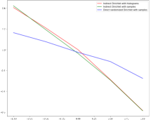

Discounting numerical errors, all estimators seem to detect convex order. The direct randomized Dirichlet method is less complex; however it does not seem to explore the -space as well as the two indirect Dirichlet methods. On the other hand, both of the indirect Dirichlet methods yield very similar results for the examples considered. As the name suggests, the “indirect Dirichlet method with samples” works on samples directly, which might be more convenient for practical applications on real data.
As can be expected from the numerical implementation, the histogram method consistently yields the lowest runtimes, while runtimes of the other methods are much higher. Indeed, when working with samples, the weights of the empirical distributions are constant, while the OT cost matrices and in the implementation have to re-computed in each iteration and this is very costly; for the histogram method, the weights change, while the grid stays constant — and thus also and .
5. Model independent arbitrage strategies
Let us consider a financial market with financial assets and denote its price process by . Let us assume and fix two maturities . If call options with these maturities are traded at all strikes, then the prices of the call options determine the distribution of and under any martingale measure; this fact was first established by Breeden and Litzenberger (1978). Let us denote the laws of and by and respectively. If trading is only allowed at and , the following definition is natural and will be crucial for our analysis.
Definition 5.1.
The triple of measurable functions is a model-independent arbitrage if , and
If no such strategies exist, then we call the market free of model-independent arbitrage.
In the above, and can be interpreted as payoffs of Vanilla options with market prices and respectively, while the term denotes the gains or losses from buying assets at time and holding them until .
The following theorem makes the connection between model-independent arbitrages and convex order of and apparent. It can essentially be found in (Guyon et al., 2017, Theorem 3.4).
Theorem 5.2.
The following are equivalent:
-
(i)
The market is free of model-independent arbitrage.
-
(ii)
.
-
(iii)
.
In particular, if , then there exists a convex function , such that the triple is a model-independent arbitrage. Here is a measurable selector of the subdifferential of .
The strategy is often called a calendar spread. As our setting is not quite exactly covered by (Guyon et al., 2017, Theorem 3.4) and the proof is not hard, we include it here.
Proof of Theorem 5.2.
(ii)(iii) is Strassen’s theorem, see Strassen (1965). If , then by definition there exists a convex function such that
On the other hand, is convex and thus satisfies
Combining the two equations above shows that is a model-independent arbitrage, and thus (i)(iii). It remains to show (ii)(i), which is well known. Indeed, taking expectations in the inequality
under any martingale measure with marginals leads to a contradiction. This concludes the proof. ∎
As a direct consequence of Theorem 5.2, we can use Theorem 1.1 to detect model-independent arbitrages in the market under consideration: indeed, Theorem 1.1 states that implies existence of a probability measure satisfying
Next, if , then the proof of Theorem 1.1 shows that for some convex function and
In particular, a model-independent arbitrage strategy is given by calendar spread . Via an approximation argument, this result remains true for arbitrary probability measures . In particular, we can use the same methods as in Section 4 to find . We then estimate from the optimizing transport plan of by taking the conditional expectation , where denotes the conditional probability distribution of with respect to its second marginal . This is a standard technique (see e.g. Deb et al. (2021) for details). In conclusion we can obtain an explicit arbitrage strategy.
To illustrate the ideas outlined above, we return to Example 4.1, i.e. and for and . Having determined such that , we estimate numerically. We show estimates for and in the plots below.


6. Remaining proofs
Proof of Corollary 2.3.
Recall that a function is -concave, iff is convex. In particular
By (10) we obtain
This concludes the proof. ∎
Proof of Corollary 2.4.
Proof of Corollary 2.1.
First, (Wang et al., 2020, Theorem 2 & Lemma 1) show that iff
| (11) |
for all concave functions such that the above integral is finite. As any concave function is Lebesgue-almost surely differentiable, standard approximation arguments imply that (11) holds iff
for all bounded increasing left-continuous functions . But
is exactly the set of all bounded increasing left-continuous functions on . Noting that by (Villani, 2003, Equation (2.47))
we calculate
This concludes the proof. ∎
References
- Acciaio et al. [2013] B. Acciaio, M. Beiglböck, F. Penkner, and W. Schachermayer. A model-free version of the Fundamental Theorem of Asset Pricing and the Super-replication Theorem. Math. Finance, DOI: 10.1111/mafi.12060, 2013.
- Alfonsi and Jourdain [2020] A. Alfonsi and B. Jourdain. Squared quadratic Wasserstein distance: optimal couplings and Lions differentiability. ESAIM Prob. Stat., 24:703–717, 2020.
- Alfonsi et al. [2019] A. Alfonsi, J. Corbetta, and B. Jourdain. Sampling of one-dimensional probability measures in the convex order and computation of robust option price bounds. Int. J. Theor. Appl. Finance, 22(3), 2019.
- Alfonsi et al. [2020] A. Alfonsi, J. Corbetta, and B. Jourdain. Sampling of probability measures in the convex order by Wasserstein projection. Ann. Henri Poincare, 56(3):1706–1729, 2020.
- Arnold [2012] B. Arnold. Majorization and the Lorenz order: A brief introduction, volume 43. Springer Science & Business Media, 2012.
- Beiglböck et al. [2013] M. Beiglböck, P. Henry-Labordère, and F. Penkner. Model-independent bounds for option prices—a mass transport approach. Finance Stoch., 17(3):477–501, 2013.
- Beiglböck et al. [2015] M. Beiglböck, M. Nutz, and N. Touzi. Complete duality for martingale optimal transport on the line. Ann. Prob., 45(5):3038–3074, 2015.
- Bernard et al. [2017] C. Bernard, L. Rüschendorf, and S. Vanduffel. Value-at-risk bounds with variance constraints. J. Risk Insur., 84(3):923–959, 2017.
- Breeden and Litzenberger [1978] D. Breeden and R. Litzenberger. Prices of state-contingent claims implicit in option prices. Journal of Business, pages 621–651, 1978.
- Brenier [1991] Y. Brenier. Polar factorization and monotone rearrangement of vector-valued functions. Commu. Pure Appl. Math., 44(4):375–417, 1991.
- Carlier [2008] Guillaume Carlier. Remarks on toland’s duality, convexity constraint and optimal transport. Pacific Journal of Optimization, 4(3):423–432, 2008.
- De March and Touzi [2019] H. De March and N. Touzi. Irreducible convex paving for decomposition of multidimensional martingale transport plans. Ann. Prob., 47(3):1726–1774, 2019.
- Deb et al. [2021] Nabarun Deb, Promit Ghosal, and Bodhisattva Sen. Rates of estimation of optimal transport maps using plug-in estimators via barycentric projections. Advances in Neural Information Processing Systems, 34:29736–29753, 2021.
- Embrechts et al. [2013] P. Embrechts, G. Puccetti, and L. Rüschendorf. Model uncertainty and var aggregation. J. Bank. Financ., 37(8):2750–2764, 2013.
- Galichon et al. [2014] A. Galichon, P. Henry-Labordère, and N. Touzi. A stochastic control approach to no-arbitrage bounds given marginals, with an application to lookback options. Ann. Appl. Prob., 24(1):312–336, 2014.
- Guo and Obłój [2019] Gaoyue Guo and Jan Obłój. Computational methods for martingale optimal transport problems. Ann. Appl. Prob., 29(6):3311–3347, 2019.
- Guyon et al. [2017] Julien Guyon, Romain Menegaux, and Marcel Nutz. Bounds for VIX futures given S&P 500 smiles. Finance and Stochastics, 21:593–630, 2017.
- Jourdain and Margheriti [2022] B. Jourdain and W. Margheriti. Martingale Wasserstein inequality for probability measures in the convex order. Bernoulli, 28(2):830–858, 2022.
- Kantorovich [1958] L. Kantorovich. On the translocation of masses. Manag. Sci., (5):1–4, 1958.
- Massa and Siorpaes [2022] M. Massa and P. Siorpaes. How to quantise probabilities while preserving their convex order. arXiv preprint arXiv:2206.10514, 2022.
- Monge [1781] G. Monge. Mémoire sur la théorie des déblais et des remblais. De l’Imprimerie Royale, 1781.
- Müller and Stoyan [2002] A. Müller and D. Stoyan. Comparison methods for stochastic models and risks, volume 389. Wiley, 2002.
- Nendel [2020] M. Nendel. A note on stochastic dominance, uniform integrability and lattice properties. Bull. Lond. Math. Soc., 52(5):907–923, 2020.
- Obłój and Siorpaes [2017] J. Obłój and P. Siorpaes. Structure of martingale transports in finite dimensions. arXiv preprint arXiv:1702.08433, 2017.
- Peyré and Cuturi [2019] G. Peyré and M. Cuturi. Computational optimal transport: With applications to data science. Foundations and Trends® in Machine Learning, 11(5-6):355–607, 2019.
- Rachev and Rüschendorf [1998] S. Rachev and L. Rüschendorf. Mass Transportation Problems: Volume I: Theory, volume 1. Springer Science Business Media, 1998.
- Ross et al. [1996] S. M Ross, J. Kelly, R. Sullivan, W. Perry, D. Mercer, R. Davis, T. Washburn, E. Sager, J. Boyce, and V. Bristow. Stochastic processes, volume 2. Wiley New York, 1996.
- Rüschendorf and Rachev [1990] L. Rüschendorf and S. Rachev. A characterization of random variables with minimum L2-distance. J. Multivariate Anal., 32(1):48–54, 1990.
- Rüschendorf and Uckelmann [2002] L. Rüschendorf and L. Uckelmann. Variance minimization and random variables with constant sum. In et al. Cuadras, editor, Distributions with given marginals and statistical modelling, pages 211–222. Springer, 2002.
- Shaked and Shanthikumar [2007] M. Shaked and J. Shanthikumar. Stochastic orders. Springer, 2007.
- Strassen [1965] V. Strassen. The existence of probability measures with given marginals. Ann. Math. Statist., pages 423–439, 1965.
- Tchen [1980] A. Tchen. Inequalities for distributions with given marginals. Ann. Prob., pages 814–827, 1980.
- Villani [2003] C. Villani. Topics in optimal transportation. Number 58. American Mathematical Soc., 2003.
- Villani [2008] C. Villani. Optimal transport: old and new, volume 338. Springer Berlin, 2008.
- Wang and Wang [2011] B. Wang and R. Wang. The complete mixability and convex minimization problems with monotone marginal densities. J. Multivariate Anal., 102(10):1344–1360, 2011.
- Wang et al. [2020] Q. Wang, R. Wang, and Y. Wei. Distortion riskmetrics on general spaces. Astin Bull., 50(3):827–851, 2020.