An LMI Framework for Contraction-based Nonlinear Control Design by Derivatives of Gaussian Process Regression
Abstract
Contraction theory formulates the analysis of nonlinear systems in terms of Jacobian matrices. Although this provides the potential to develop a linear matrix inequality (LMI) framework for nonlinear control design, conditions are imposed not on controllers but on their partial derivatives, which makes control design challenging. In this paper, we illustrate this so-called integrability problem can be solved by a non-standard use of Gaussian process regression (GPR) for parameterizing controllers and then establish an LMI framework of contraction-based control design for nonlinear discrete-time systems, as an easy-to-implement tool. Later on, we consider the case where the drift vector fields are unknown and employ GPR for functional fitting as its standard use. GPR describes learning errors in terms of probability, and thus we further discuss how to incorporate stochastic learning errors into the proposed LMI framework.
keywords:
Nonlinear systems, discrete-time systems, stochastic systems, contraction analysis, Gaussian process regression1 Introduction
Contraction theory [28, 9] has attracted massive research attention in the systems and control community, e.g., [7, 40], which establishes a differential geometric approach to study incremental properties, i.e., properties between any pair of trajectories. Revisiting nonlinear control theory from contraction perspectives brings new insights not only for stability analysis but also for dissipativity theory [43, 11, 23], balancing theory [25, 19], and monotone systems [10, 20, 21] to name a few. As an advantage in comparison with classical Lyapunov theory, the nature of incremental stability enables us to formulate various design problems in a unified framework, such as stabilizing control [29, 24], tracking control [15, 33], observer design [1, 28], and control design for achieving synchronizations [1] and other rich behaviors [11]. Owing to the differential geometric feature, these problems are described in terms of Jacobian matrices, which is expected as another advantage in practical use. Indeed, restricting the class of controllers (and observer gains) into linear reduces design problems to linear matrix inequalities (LMIs) [19, 11]. However, nonlinear control design is more involved because of the so-called integrability problem. Namely, design conditions are imposed not on controllers but on their partial derivatives, which are the main difficulty in developing an LMI framework for contraction-based nonlinear control design.
To overcome this difficulty, in this paper, we employ Gaussian process regression (GPR), a functional fitting tool [32, 4]. As its non-standard use, we employ GPR to parametrize a controller based on its two important features: 1) computing derivatives of GPR is easy; 2) GPR becomes linear with respect to parameters while it possesses the flexibility to describe a nonlinear function. Utilizing these two, we describe a condition for control design in terms of LMIs with respect to parameters of GPR. Namely, we establish an LMI framework for contraction-based nonlinear stabilizing control design by explicitly addressing the integrability problem. We mainly consider nonlinear discrete-time systems with constant input vector fields and constant metrics for contraction. Then, we mention that the formulations are still in the LMI framework for discrete-time systems with non-constant input vector fields and continuous-time systems with non-constant input vector fields and non-constant metrics. The proposed method is further applicable to the aforementioned various design problems thanks to a unified problem formulation by contraction theory.
In systems and control, GPR is typically used to estimate an unknown drift vector field from measured states, and [17, 36, 35, 2, 41, 42] study control design for learned models. Other applications are a joint estimation of the state and model [3, 6] and solving the Hamilton-Jacobi equations/inequalities [18, 14]. In particular, [35, 2, 41, 42] study closed-loop stability under learning errors. However, controllers are designed without taking learning errors into account, and learning errors are used for closed-loop analysis only. Motivated by these works, in this paper, we also consider the case where a drift vector field is unknown, and this is learned by GPR. In contrast to the conventional approach, we compensate for the learning error by control design, which are benefits of developing the LMI framework for control design and learning models by GPR. The proposed approach can be generalized to the case where the whole system dynamics are unknown, and only system’s input and output are measurable, since there are learning approaches by GPR in such a setting [13, 12].
As relevant researches, [38, 39, 35] give neural network frameworks for contraction-based control design, which requires iterations for finding suitable parameters in contrast to the proposed LMI framework. The paper [17] formulates control design for models learned by GPR in an LMI framework and designs a switching linear controller, but does not use GPR for control design or is not based on contraction theory. Therefore, the result in [17] is not applicable for solving the integrability problem. In this paper, we establish an LMI framework for contraction-based control design by utilizing the derivatives of GPR to solve the integrability problem.
The remainder of this paper is organized as follows. In Section 2, we pose the problem formulation by mentioning the integrability problem of control design in contraction theory. In Section 3, we develop an LMI framework for contraction-based control design by utilizing derivatives of GPR. In Section 4, we consider the case where drift vector fields are unknown. In Section 5, the proposed control design method is illustrated by the means of an example.
Notation: The sets of real numbers, non-negative integers, and positive integers are denoted by , , and , respectively. The identity matrix with the size is denoted by . For , (resp. ) means that is symmetric and positive definite (resp. semi-definite). The Euclidean norm of weighted by is denoted by . If , this is simply denoted by . The Moore-Penrose inverse of a matrix is denoted by .
For a function , the row vector-valued function consisting of its partial derivatives with respect to is denoted by . If depends on only, this is simply denoted by . For a scalar-valued function , its Hessian matrix is denoted by , which is a matrix-valued function. The multivariate normal distribution with mean and variance is denoted by . The (standard) expectation is denoted by . A stochastic process is said to be i.i.d. if , are independently distributed, and none of the characteristics of changes with .
2 Preliminaries
2.1 Problem Formulation
Consider the following discrete-time nonlinear system:
| (1) |
where and denote the state and input, respectively; is of class , i.e., continuously differentiable, and . The th components of and are denoted by and , respectively. For the sake of notational simplicity, we consider single-input systems. However, the results can readily be generalized to multiple-input systems as explained below. We also later discuss the case where is a function of .
In contraction theory [28, 37, 22], we study incremental stability as a property of the pair of trajectories, stated below.
Definition 2.1.
The system (with its copy ) is said to be incrementally exponentially stable (IES) if there exist and such that
for each .
Applying [37, Theorem 15] to control design yields the following IES condition.
Proposition 2.2.
Suppose that there exist , , and of continuous such that
| (2) |
for all , where represents the appropriate matrix. If there exists of class such that
| (3) |
for all , then the closed-loop system is IES.
By the Schur complement, the set of (2) and (3) is equivalent to and
| (4) |
This is nothing but the definition of uniform contraction with [37, Definition 6] for the closed-loop system . Therefore, [37, Theorem 15] concludes IES of the closed-loop system. ∎
In [37, Theorem 15], it has been shown that a closed IES system admits a state-dependent satisfying a similar inequality as (2). Moreover, such a is uniformly lower and upper bounded by constant matrices. It is not yet clear when becomes constant. If one restricts the class of controllers into linear for a constant , control design can be reduced to linear matrix inequalities (LMIs); see, e.g., [11, 19]. Namely, control design can be sometimes formulated as a practically solvable problem even for nonlinear systems. Indeed, (2) is an LMI with respect to , and at each . However, as in Proposition 2.2, designing nonlinear controllers is not fully formulated in the LMI framework, due to the so-called integrability constraint (3), i.e., needs to be the partial derivative of some function providing a feedback control law . The main objective of this paper is to develop an LMI framework for stabilizing nonlinear control design by tackling the integrability constraint, stated below.
Problem 2.3.
Remark 2.4.
We later consider the case where is unknown by learning it. As a byproduct of developing control design methodologies in the LMI framework, it is possible to compensate for learning errors by control design.
An important feature of contraction theory is to study the convergence between any pair of trajectories. By virtue of this, one can handle observer design [1, 28], tracking control [15, 33], and control design for imposing synchronizations [1] and rich behavior such as limit cycles [11] in the same framework as stabilizing control design. These references mainly focus on continuous-time systems, but similar results can be delivered to discrete-time systems, since incremental stability conditions in contraction analysis have been derived also for discrete-time systems [28, 37]. Moreover, the proposed method in this paper can be generalized to continuous-time systems as will be explained in Section 3.3. Therefore, solving Problem 2.3 can result in LMI frameworks for various design problems.
Integrability constraints sometimes appear in nonlinear adaptive control or observer design. Since directly addressing integrability constraints are difficult, there are techniques for avoiding them by adding the dynamic order of the identifier. However, as pointed out by [27], adding additional dynamics can degenerate control performances, and it has not been validated that such an approach works for contraction-based control design. Therefore, it is worth solving Problem 2.3 directly. In particular, we provide an LMI framework for control design, which is easy-to-implement. The proposed method may be tailored for nonlinear adaptive control or observer design although this is beyond the scope of this paper.
2.2 Gaussian Process Regression
To solve Problem 2.3, we employ Gaussian process regression (GPR) [32, 4]. We, in this subsection, briefly summarize basics of GPR and, in the next section, demonstrate that GPR is a suitable tool for handling problems involving partial derivatives, e.g., integrability conditions.
Let , be input data, and let , be the corresponding output data given by
| (5) |
where is i.i.d. GPR is a technique to learn an unknown function from input-output data by assuming as a Gaussian process (GP).
A stochastic process is said to be GP if any finite set has a joint Gaussian distribution [32, Definition 2.1]. A GP is completely specified by its mean function and covariance function . They are defined by
| (6) | ||||
| (7) |
and we represent the GP by .
The essence of GPR is to estimate and as the posterior mean and covariance given by the Bayes estimation [32, 4]. Typically, the prior mean is selected as zero. The prior covariance needs to be a positive definite kernel [32, Section 6], and we also require smoothness. Standard kernels are linear, polynomial, or squared exponential (SE) [32, 4], which are all smooth and positive definite. For instance, an SE kernel is
| (8) |
where and in addition to in (5) are free parameters, called hyper parameters. The hyper parameters can be selected to maximize the marginal likelihood from observed data; see e.g., [32, Section 5.4].
3 Contraction-based Nonlinear Control Design
In this section, we establish an LMI framework for contraction-based nonlinear control design by utilizing derivatives of GPR to solve the integrability problem. Then, we discuss generalizations of the proposed method to non-constant input vector fields and continuous-time cases.
3.1 LMI Frameworks for Nonlinear Control Design
Taking the partial derivatives of (6) and (7), we have the joint distribution of and as in
| (9) |
see, e.g., [30, Equation (2)]. The goal of this subsection is to find based on the Bayes estimation such that is a solution to Problem 2.3. For the sake of notational simplicity, we select the prior mean of as zero.
A standard procedure of the Bayes estimation is that we first select a class positive definite kernel as a prior covariance. Then, we compute the posterior mean given data of . Looking at this from a different angle, can be viewed as a function of data of . Based on this perspective, we consider generating suitable data such that becomes a solution to Problem 2.3 as a non-standard use of GPR.
To this end, let denote a data set to be generated, where
| (10) |
The role of i.i.d. is explained later; one can simply choose it as zero. Define the vector consisting of by
Also, we introduce the following notations:
| (11) |
Then, the joint distribution of the prior distribution of , denoted by and is
By the Bayes estimation, we can compute the posterior mean given as
| (12) |
where denotes the th block-component with size of defined by
| (13) |
The partial derivative of is easy-to-compute:
| (14) |
Especially if and , it follows from (14) that
| (15) |
Note that and are nonlinear functions of and linear functions of . Therefore, control design reduces to generating suitable , i.e., , which is proceeded based on Proposition 2.2.
Now, we are ready to develop an LMI framework for contraction-based nonlinear control design. Substituting into (2) does not give an LMI because of the coupling between and . This issue can be addressed by using a standard technique of an LMI. According to [34, Theorem 2.3.11], (2), i.e., the set of and (2.1) implies, for all ,
| (18) |
This is an LMI with respect to and at each . For a solution to (18) and , one only has to solve (2) with respect to . The proposed procedure for solving Problem 2.3 is summarized in Algorithm 1.
If Algorithm 1 has a set of solutions, the obtained is a solution to Problem 2.3 at each data point, stated below.
Theorem 3.1.
Using a set of solutions and , define . Then, (3) holds for all . It suffices to confirm that (2) holds at , . Since , we have , . Therefore, (23) implies (2) for , . ∎
Note that in Algorithm 1, the number of training data and data point set can be chosen arbitrarily. As increases, the number of in (23) increase. However, the problem is still convex. As explained in the next subsection, for sufficiently large , one can show that is a solution to Problem 2.3 other than when is distributed evenly in the state space. Moreover, such can be found.
When and , (15) helps to simplify Algorithm 1. In fact, we only have to solve a finite family of LMIs once, stated below without the proof.
Corollary 3.2.
Remark 3.3.
It is not guaranteed that the constructed controller in Theorem 3.1 preserves an equilibrium point of . However, it is easy to impose . An approach is to use shifted . Another approach is to utilize (5). Consider new data in (5). Define . Then, the posterior mean given and can be computed by the Bayes estimation also. As a special case, specifying , , , and can result for learned . More generally, one can specify the values of at arbitrary finite points .
Remark 3.4.
In the multiple-input case, each component of can be designed separately by introducing corresponding to . Namely, the results obtained in this paper can readily be generalized to the multiple-input case.
At the end of this subsection, we argue the role of in (10) by interpreting the procedure of Algorithm 1 as follows. We generate suitable based on the LMIs and then construct by functional fitting. In functional fitting, overfitting is a common issue, since a constructed function becomes unnecessarily complex. The variance specifies how much a constructed function needs to fit to data, and thus adding the noise helps to avoid overfitting. However, if is large, a constructed function can fit to instead of . This is well known as the bias-variance tradeoff in functional fitting [16, Section 5.4.4]. It is worth emphasizing that Theorem 3.1 holds for arbitrary .
If in (11) is non-singular, in (13) is nothing but the minimizer of the following optimization problem:
| (25) |
The first term evaluates the fitting error at each and the second one is for regularization. Especially when , the optimal value becomes zero for the obtained , i.e., a complete fitting , is achieved as stated by Corollary 3.2. A reproducing kernel Hilbert space is a formal tool to study a functional fitting problem under regularization as an optimization problem. For the prior variance as a kernel, the pair can be understood as a minimizer according to the representer theorem [31, Theorem 2].
3.2 Closed-loop Stability
In Theorem 3.1, it is not clear whether satisfies (2) other than in contrast to the integrability condition (3). Applying standard arguments of the polytope approach [5], we improve the LMIs in Algorithm 1 such that its solution satisfies (2) other than when is sufficiently large.
For a set of matrices , let denote its convex hull, i.e.,
Now, we choose and
From the standard discussion of the polytope approach [5], (2) and (3) hold for all belonging to
This set can be made larger by increasing the number of data used for control design.
Increasing is not the only approach to enlarge a set of in which (2) holds. Another approach is to improve the LMIs in Algorithm 1. First, we decide which is arbitrary as long as
| (26) |
Instead of (21), we consider the following finite family of LMIs with respect to and :
| (29) | |||
Using a solution , we consider the following finite family of LMIs with respect to and instead of (23):
| (30) | |||
The newly obtained satisfies (2) for all belonging to
Now, we are ready to state a control design procedure such that the IES conditions (2) and (3) hold on a given bounded set.
Theorem 3.5.
Consider a system (1), a class positive definite kernel , and . Let denote an -dimensional closed hypercube. We partition it evenly to closed hypercubes, denoted by , where , . For all , there exist , such that
| (31) | ||||
Let each , be the center of . Suppose that for such , ,
-
1)
for all , the LMI (29) admits and ;
-
2)
for all and obtained in item 1), the LMI (30) admits and ;
-
3)
for the elements of , there exists a strictly decreasing positive function of such that as , and if and are next to each other.
Then, there exists a sufficiently large such that satisfies (2) and (3) for all .
First, we show (31). Since a continuous function is bounded on a bounded set, is bounded for each . Each bounded set admits its convex hull. Therefore, there exists satisfying (31).
Next, we consider the latter statement. We choose . Then, (3) holds on . It remains to show that (2) holds on . Items 1) and 2) and (31) imply that for each ,
The strict inequality holds for any positive . Since is continuous (with respect to ), there exists a sufficiently small centered at such that
From item 3), the continuity of and , and the boundedness of , there exists a sufficiently large such that for all . Consequently, (2) hold on , a union of , . ∎
In the above theorem, and are not necessarily to be hypercubes or closed. Essential requirements are that is covered by , and each shrinks as increases. In the proof, we show that a switching controller , also satisfies (2) and (3). However, a continuous controller is more easy-to-implement.
Remark 3.6.
In Theorem 3.5, IES of the closed-loop system is guaranteed on geodesically convex if either is positively invariant or contains an equilibrium point. By the Schur complement, one can confirm that (2) and (3) on implies (2.1) on . According to the proof of [37, Theorem 15], if (2.1) holds on , then there exists such that
for all and as long as . This implies that if is geodesically convex and positively invariant, the closed-loop system is IES on . Next, if contains an equilibrium point , it follows that
for all . From geodesic convexity, this further implies that is positively invariant. Thus, the closed-loop system is IES on .
3.3 Discussions for Generalizations
In this subsection, we discuss how to generalize our results to the cases where the input vector field is a function of . Also, we mention the continuous-time case.
First, we consider the system with non-constant :
| (32) |
where is of class . A modification of Proposition 2.2 implies that a controller achieves IES if there exist , , and of class such that for all ,
| (33) |
The difference from (2) is the additional term .
For finding first, one can utilize a modification of (18):
| (36) |
Substituting its solution , , and into (33) yields an LMI with respect to and at each . Therefore, even for non-constant , one can still design a controller only by solving two finite families of LMIs on data points .
In this paper, we focus on discrete-time systems. However, our method can also be applied to the continuous-time systems:
| (37) |
According to [9, Theorem 1], a controller makes the closed-loop system IES if there exist and , such that for all ,
| (38) | ||||
Let and , where denotes the th element of , and is i.i.d. Denote by the posterior mean of given , . Then, we first find satisfying and
For the obtained , it suffices to solve (3.3) with respect to , i.e., . Therefore, in the continuous-time case, nonlinear control design can be achieved only by solving two finite families of LMIs at even for a non-constant metric . As mentioned in Section 2.1, the proposed method can further be applied to various design problems.
4 Control Design for Unknown Systems
For unknown system dynamics, it is shown by e.g. [13, 12] that its state-space model can be estimated from the system’s input and output by GPR. Since GPR is a Bayesian approach, the estimation error is represented by a posterior covariance. In this section, we show how to compensate for a stochastic learning error by control design. To focus on exposing the main idea, we consider a case where the drift vector field is unknown, and the state is measurable, but the results can be generalized to the case where all systems dynamics are unknown and only the system’s input and output are measurable by utilizing the results in [13, 12].
4.1 Learning Drift Vector Fields
In GPR, we learn each component , of separately from training data ,
where is i.i.d. The number of training data and training data points for learning are allowed to be different from those used for control design. Differently from control design, we can directly obtain training data of , and thus it can be estimated by the standard use of GPR. Moreover, to compensate for the learning error of by control design, we estimate the error as the posterior covariance.
We choose a prior distribution of as , where is a class positive definite kernel. Then, the Bayes estimation yields the posterior mean of the joint distribution of and as follows:
where denotes the th component of ; see, e.g. [32, Section 2] for the computation of , and can be computed by taking its partial derivative with respect to .
Remark 4.1.
When is also unknown, we learn , from training data ,
To utilize the prior knowledge that is linear with respect to , we employ the following kernel , where is a class positive definite kernel. Namely, we select a prior distribution of as . Then, the Bayes estimation yields the posterior mean of as follows:
where and are the same as the above. Note that is linear with respect to .
A benefit of GPR for learning a function is the ease of analytical computation of the posterior covariance function of as in
Similarly, the posterior covariance function of is easy to compute:
Therefore, the posterior distributions of and are respectively obtained by
and consequently,
| (39) |
An advantage of obtaining the covariance functions and in nonlinear system identification is that one can compute empirical confidence intervals and decide if one increases training data in some region of interest to relearn the model. Repeating this, one can construct a model with a desired accuracy.
Taking the model learning error into account, a representation of an estimated closed-loop system with becomes
| (40) | |||
where is i.i.d. The error can be compensated by control design. To see this, we study the stochastic system (40) from two aspects. First, by applying a moment IES condition in [22, Corollary 5.4], we argue how to choose in the LMI (23). Then, we also discuss how to construct , for guaranteeing IES in probability.
4.2 Moment Incremental Stability
Proposition 2.2 for IES has been generalized to the moment IES of stochastic systems [22, Corollary 5.4]. This can be used to decide in (23) for control design.
Definition 4.2.
Proposition 4.3.
A system (40) is IES in the second moment if there exist and such that
| (44) |
for all , where each , denotes the standard basis whose th element is , and the other elements are all .
4.3 Incremental Stability in Probability
In Section 3.2 for control design, a polytope approach has been mentioned. There is a freedom to design finite families of matrices , . This can be utilized to guarantee IES in probability.
Applying the Chebyshev’s inequality [8, Theorem 1] yields, given ,
where is the variance of the Jacobian matrix, computed in (39). Therefore, one can design such that is contained in in probability , where note that and , are mutually independent. For the designed , suppose that (30) has a set of solutions. Then, a controller guaranteeing IES in probability can be constructed from the solutions.
5 Example
Consider a negative resistance oscillator [26, Exercise 2.7]. Its forward Euler discretization with the sampling period is given by
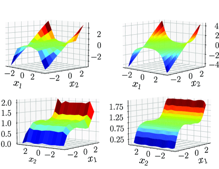
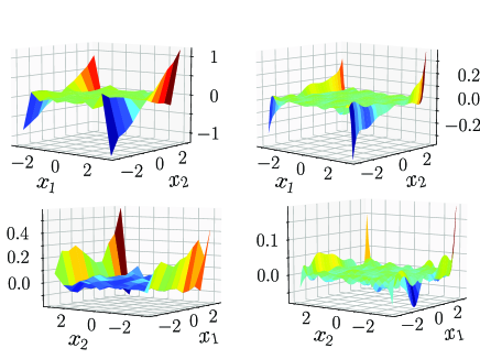
We learn only, since is determined by the psychical structure. For the number of training data, we consider two cases and . For both cases, training data points are equally distributed on . Training data is generated by , where . As a kernel function, we use a Gaussian kernel . Figures 1 and 2 show the learned and the learning error , respectively. In Fig. 2, the error is large around the edges. This is because when computing derivatives at some point, we need information around it, but around the edges, this is not possible. In other words, the learned in Fig. 1 is closed to the true except for the edges.
(left) (right)
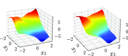
Next, we design a nonlinear controller based on the learned by using Algorithm 1. To avoid the edges, we consider a smaller region . For the number of training data, we consider two cases and . For both cases, training data points are equally distributed. We select and . Then, for both cases, solutions to the LMI (21) are the same:
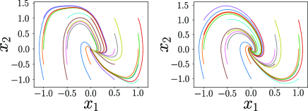
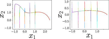
For this , we solve the LMI (23) and construct that is plotted in Fig. 3. We apply the constructed controller to the true system. Since the origin is an equilibrium point of , we modify the controller as to preserve the equilibrium point. For the different numbers of training data, Fig. 4 shows the phase portraits of the closed-loop systems, i.e., the state trajectories starting from different initial states. In each case, the origin of the true system is stabilized by a controller designed for a learned model.
An advantage of our approach is that a nonlinear stabilizing controller is designed only by solving LMIs. The papers [41, 42] propose stabilizing control design methods for a model learned by GPR. The essence of these methods are to cancel nonlinear terms by state feedback like feedback linearization. We apply this approach. Namely, we divide control design procedure into two steps. First, we apply for cancelling the nonlinear term , where is an estimation of . Next, we design linear feedback based on the linear terms, which can be done by solving an LMI. In fact, we obtain . For the different numbers of training data, Fig 5 shows the phase portrait of the closed-loop system by . In each case, some trajectories (e.g. the red colored one) does not converge to the equilibrium point. This can be caused by the gap between true and learned as known that feedback linearization is weak at model uncertainty.
6 Conclusion
In this paper, we have established an LMI framework for contraction-based control design by utilizing the derivatives of GPR to solve the integrability problem, as an easy-to-implement tool for nonlinear control. Differently from the standard use, we have used GPR to parametrize a set of controllers and have found suitable parameters from the contraction condition. The proposed method can further deal with the case where system dynamics are unknown by learning them by GPR, and the learning errors can be compensated by control design by simple modifications of the proposed LMI framework. Future work includes applying our method to a high-dimensional model with a real data set.
References
- [1] V. Andrieu, B. Jayawardhana, and L. Praly. Transverse exponential stability and applications. IEEE Transactions on Automatic Control, 61(11):3396–3411, 2016.
- [2] T. Beckers, D. Kulić, and S. Hirche. Stable Gaussian process based tracking control of Euler–Lagrange systems. Automatica, 103:390–397, 2019.
- [3] K. Berntorp. Online Bayesian inference and learning of Gaussian-process state–space models. Automatica, 129:109613, 2021.
- [4] C. M. Bishop. Pattern Recognition and Machine Learning. Springer, New York, 2006.
- [5] S. Boyd, L. El Ghaoui, E. Feron, and V. Balakrishnan. Linear Matrix Inequalities in System and Control Theory. SIAM, Philadelphia, 1994.
- [6] M. Buisson-Fenet, V. Morgenthaler, S. Trimpe, and F. Di Meglio. Joint state and dynamics estimation with high-gain observers and Gaussian process models. IEEE Control Systems Letters, 5(5):1627–1632, 2020.
- [7] F. Bullo. Contraction Theory for Dynamical Systems. Kindle Directed Publishing, 2022.
- [8] X. Chen. A new generalization of Chebyshev inequality for random vectors. arXiv:0707.0805, 2007.
- [9] F. Forni and R. Sepulchre. A differential Lyapunov framework for contraction anlaysis. IEEE Transactions on Automatic Control, 59(3):614–628, 2014.
- [10] F. Forni and R. Sepulchre. Differentially positive systems. IEEE Transactions on Automatic Control, 61(2):346–359, 2015.
- [11] F. Forni and R. Sepulchre. Differential dissipativity theory for dominance analysis. IEEE Transactions on Automatic Control, 64(6):2340–2351, 2018.
- [12] R. Frigola, Y. Chen, and C.E. Rasmussen. Variational Gaussian process state-space models. Advances in Neural Information Processing Systems, 27, 2014.
- [13] R. Frigola, F. Lindsten, T.B. Schön, and C.E. Rasmussen. Identification of Gaussian process state-space models with particle stochastic approximation EM. IFAC Proceedings Volumes, 47(3):4097–4102, 2014.
- [14] K. Fujimoto, H. Beppu, and Y. Takaki. On computation of numerical solutions to Hamilton-Jacobi inequalities using Gaussian process regression. Proc.2018 American Control Conference, pages 424–429, 2018.
- [15] M. Giaccagli, D. Astolfi, V. Andrieu, and L. Marconi. Sufficient conditions for global integral action via incremental forwarding for input-affine nonlinear systems. IEEE Transactions on Automatic Control, 67(12):6537 – 6551, 2022.
- [16] I. Goodfellow, Y. Bengio, and A. Courville. Deep Learning. MIT press, Massachusetts, 2016.
- [17] Y. Ito, K. Fujimoto, Y. Tadokoro, and T. Yoshimura. On stabilizing control of Gaussian processes for unknown nonlinear systems. IFAC-PapersOnLine, 50(1):15385–15390, 2017.
- [18] Y. Ito, K. Fujimoto, T. Yoshimura, and Y. Tadokoro. On Gaussian kernel-based Hamilton-Jacobi-Bellman equations for nonlinear optimal control. Proc.2018 American Control Conference, pages 1835–1840, 2018.
- [19] Y. Kawano. Controller reduction for nonlinear systems by generalized differential balancing. IEEE Transactions on Automatic Control, 67(11):5856–5871, 2022.
- [20] Y. Kawano, B. Besselink, and M. Cao. Contraction analysis of monotone systems via separable functions. IEEE Transactions on Automatic Control, 65(8):3486–3501, 2020.
- [21] Y. Kawano and M. Cao. Contraction analysis of virtually positive systems. Systems & Control Letters, 168:105358, 2022.
- [22] Y. Kawano and Y. Hosoe. Contraction analysis of discrete-time stochastic systems. arXiv:2106.05635, 2021.
- [23] Y. Kawano, C. K. Kosaraju, and J. M. A. Scherpen. Krasovskii and shifted passivity based control. IEEE Transactions on Automatic Control, 66(10):4926–4932, 2021.
- [24] Y. Kawano and T. Ohtsuka. Nonlinear eigenvalue approach to differential Riccati equations for contraction analysis. IEEE Transactions on Automatic Control, 62(10):6497– 6504, 2017.
- [25] Y. Kawano and J. M. A. Scherpen. Model reduction by differential balancing based on nonlinear Hankel operators. IEEE Transactions on Automatic Control, 62(7):3293–3308, 2017.
- [26] H. K. Khalil. Nonlinear Systems. Prentice-Hall, New Jersey, 1996.
- [27] M. Krstic. On using least-squares updates without regressor filtering in identification and adaptive control of nonlinear systems. Automatica, 45(3):731–735, 2009.
- [28] W. Lohmiller and J.-J. E. Slotine. On contraction analysis for non-linear systems. Automatica, 34(6):683–696, 1998.
- [29] I. R. Manchester and J.-J. E. Slotine. Control contraction metrics: Convex and intrinsic criteria for nonlinear feedback design. IEEE Transactions on Automatic Control, 62(6):3046–3053, 2017.
- [30] M. Padidar, X. Zhu, L. Huang, J. Gardner, and D. Bindel. Scaling gaussian processes with derivative information using variational inference. Advances in Neural Information Processing Systems, 34, 2021.
- [31] G. Pillonetto, F. Dinuzzo, T. Chen, G. De Nicolao, and L. Ljung. Kernel methods in system identification, machine learning and function estimation: A survey. Automatica, 50(3):657–682, 2014.
- [32] C. E. Rasmussen and C. K. I. Williams. Gaussian Processes for Machine Learning. MIT Press, Massachusetts, 2006.
- [33] R. Reyes-Báez, A. J. van der Schaft, and B. Jayawardhana. Tracking control of fully-actuated port-Hamiltonian mechanical systems via sliding manifolds and contraction analysis. Proc. 20th IFAC World Congress, pages 8256–8261, 2017.
- [34] E. S. Robert, T. Iwasaki, and M. G. Karolos. A Unified Algebraic Approach to Linear Control Design. Routledge, London, 2017.
- [35] D. Sun, M. J. Khojasteh, S. Shekhar, and C. Fan. Uncertain-aware safe exploratory planning using Gaussian process and neural control contraction metric. Proc. 3rd Annual Conference on Learning for Dynamics and Control, pages 728–741, 2021.
- [36] Y. Takaki and K. Fujimoto. On output feedback controller design for Gaussian process state space models. Proc.56th IEEE Conference on Decision and Control, pages 3652–3657, 2017.
- [37] D. N. Tran, B. S. Rüffer, and C. M. Kellett. Convergence properties for discrete-time nonlinear systems. IEEE Transactions on Automatic Control, 63(8):3415–3422, 2018.
- [38] H. Tsukamoto and S.-J. Chung. Convex optimization-based controller design for stochastic nonlinear systems using contraction analysis. Proc. 58th IEEE Conference on Decision and Control, pages 8196–8203, 2019.
- [39] H. Tsukamoto, S.-J. Chung, and J.-J. E. Slotine. Neural stochastic contraction metrics for learning-based control and estimation. IEEE Control Systems Letters, 5(5):1825–1830, 2020.
- [40] H. Tsukamoto, S.-J. Chung, and J.-J. E. Slotine. Contraction theory for nonlinear stability analysis and learning-based control: A tutorial overview. Annual Reviews in Control, 52:135–169, 2021.
- [41] J. Umlauft and S. Hirche. Feedback linearization based on Gaussian processes with event-triggered online learning. IEEE Transactions on Automatic Control, 65(10):4154–4169, 2019.
- [42] J. Umlauft, L. Pöhler, and S. Hirche. An uncertainty-based control Lyapunov approach for control-affine systems modeled by Gaussian process. IEEE Control Systems Letters, 2(3):483–488, 2018.
- [43] A. J. van der Schaft. On differential passivity. IFAC Proceedings Volumes, 46(23):21–25, 2013.