An Introduction to Fluid Dynamics and Numerical Solution of Shock Tube Problem by Using Roe Solver

1 Introduction

1.1 What is a Fluid?

A fluid is any substance that deforms continuously when subjected to a shear stress, no matter how small. Usually a liquid or a gas.

1.2 Newton’s Law of Viscosity:

The shear viscosity of a fluid expresses its resistance to shearing flows, where adjacent layers move parallel to each other with different speeds. It can be defined through the idealized situation known as a Couette flow, where a layer of fluid is trapped between two horizontal plates, one fixed and one moving horizontally at constant speed . (The plates are assumed to be very large, so that one need not consider what happens near their edges.)If the speed of the top plate is small enough, the fluid particles will move parallel to it, and their speed will vary linearly from zero at the bottom to at the top. Each layer of fluid will move faster than the one just below it, and friction between them will give rise to a force resisting their relative motion. In particular, the fluid will apply on the top plate a force in the direction opposite to its motion, and an equal but opposite to the bottom plate. An external force is therefore required in order to keep the top plate moving at constant speed.

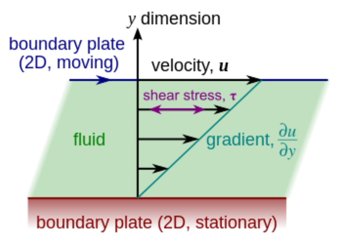
Refer to caption — Figure 1: Laminar shear of fluid between two plates.

The magnitude F of this force is found to be proportional to the speed u and the area A of each plate , and inversely proportional to the separation y. i.e.

\textbf{F}=\mu A\frac{\textbf{u}}{y}

the proportionality factor $\mu$ is this formula the viscosity of the fluid The ratio $\frac{\textbf{u}}{y}$ is called the rate of shear deformation or shear velocity, and is the derivative of the fluid speed in the direction perpendicular to the plates. Isaac Newton expressed the viscous forces by the differential equation

\tau=\mu\frac{\partial\textbf{u}}{\partial y}

where $\tau=\frac{\textbf{f}}{A}$ and $\frac{\partial\textbf{u}}{\partial y}$ is the local shear velocity. and similar case for 2 D

\tau_{xy}=\mu\left(\frac{\partial\textbf{u}}{\partial y}+\frac{\partial\textbf{v}}{\partial x}\right)

This is also known as Newton’s Second law of Viscosity.

1.3 Specification of motion

Fluids are treated as continuous media. There are four main physical idea which forms the basis of fluid dynamics:

$\ast$

The continuum hypothesis,
$\ast$

Conservation of mass,
$\ast$

Balance of momentum (Newton‘s second law of motion) and
$\ast$

Balance (conservation) of energy. The last of these is not needed in the description of some types of flows

Motion and state can be specified in terms of the velocity u, pressure P, density $\rho$ etc evaluated at every point in space x and time t. To define the density at a point, for example, suppose the point to be surrounded by a very small element (small compared with length scales of interest in experiments) which nevertheless contains a very large number of molecules. The density is then the total mass of all the molecules in the element divided by the volume of the element. Considering the velocity, pressure etc as functions of time and position in space is consistent with measurement techniques using fixed instruments in moving fluids. It is called the Eulerian specification. However, Newton’s laws of motion (see below) are expressed in terms of individual particles, or fluid elements, which move about. Specifying a fluid motion in terms of the position $\textbf{x}(t)$ of an individual particle (identified by its initial position, say) is called the Lagrangian specification. The two are linked by the fact that the velocity of such an element is equal to the velocity of the fluid evaluated at the position occupied by the element:

\frac{d\textbf{x}}{dt}=\textbf{u}(\textbf{x}(t),t)

Path Line: The path followed by a fluid element is called a particle path or path line. Mathematically obtained by

d\textbf{x}=\textbf{u}dt

\Rightarrow\textbf{x}=\textbf{x}_{0}+\int_{t_{0}}^{t_{1}}\textbf{u}(x(t),t)dt

Stream Line: A streamline is a continuous line within a fluid such that the tangent at each point is the direction of the velocity vector at that point.stream lines are defined as

\frac{d\textbf{x}}{dt}\otimes\textbf{u}=0

the components of u and x are related by from upper expression

\frac{dx}{u}=\frac{dy}{v}=\frac{dz}{dw}

Streak Lines: A streak line is the locus of the temporary locations of all particles that have passed though a fixed point in the flow field at any instant of time.

1.4 Material Derivative

Identify (or label) a material of the fluid; track (or follow) it as it moves, and monitor change in its properties. The properties may be velocity, temperature, density, mass, concentration etc in the flow field. In Lagrangian Approach the trajectory of each individual fluid parcel as it moves from some initial location, often described as “―placing a coordinate system on each fluid parcel“ and “―riding on that parcel as it travels through the fluid.“

In Eulerian Approach This corresponds to a coordinate system fixed in space, and in which fluid properties are studied as functions of time as the flow passes fixed spatial locations.

suppose a fluid property f is function of coordinate (x,y,z,t) as like f = f(x,y,z,t) and velocity vector $\textbf{U}\equiv(u,v,w)^{T}$ then

df=\frac{\partial f}{\partial t}dt+\frac{\partial f}{\partial x}dx+\frac{\partial f}{\partial y}dy+\frac{\partial f}{\partial z}dz

\Rightarrow\frac{df}{dt}=\frac{\partial f}{\partial t}+\frac{\partial f}{\partial x}\frac{dx}{dt}+\frac{\partial f}{\partial y}\frac{dy}{dt}+\frac{\partial f}{\partial z}\frac{dz}{dt}

\Rightarrow\frac{df}{dt}=\frac{\partial f}{\partial t}+u\frac{\partial f}{\partial x}+v\frac{\partial f}{\partial y}+w\frac{\partial f}{\partial z}

\Rightarrow\frac{df}{dt}=\frac{\partial f}{\partial t}+\left(\textbf{U}\cdot\nabla\right)f

the term $\frac{\partial f}{\partial t}$ is the local acceleration and $\left(\textbf{U}\cdot\nabla\right)$ the convective acceleration. The convective acceleration is nonlinear in f,which is the source of the great complexity of the mathematics and physics of fluid motion.

2 General Transport Theorem

The general transport theorem shows a beautiful equation from which the all conservation equations can be derived. This equation gives a expression for the variation of a physical quantity distributed in a scalar or vectorial field inside a deformable volume. This deformable volume can have variable mass if its boundary is permeable (open system). The basic Reynolds Transport Theorem shows the relation for a constant mass volume and a fixed volume, but it can be easily expanded to consider changes in a generic volume. The most interesting fact about these theorem is that it is only a geometrical relation. Physics only gets into the transport theorem when we define changes in a constant mass volume, which can use known physical laws, specially from thermodynamics.

2.1 Control System

Control Mass:

1.

It is a system of fixed mass.
2.

This type of system is usually referred to as “closed system”.
3.

There is no mass transfer across the system boundary.
4.

Energy transfer may be take place into or out of the system.

Control Volume:

1.

It is a system of fixed Volume.
2.

This type of system usually referred to as “Open System” or a ”Control Volume“.
3.

Mass transfer take place across the control volume.
4.

Energy Transfer also occur into or out of the system.

2.2 Reynolds Transport Theorem:

The question arise as to how a given quantity changes $\psi$ (where, $\psi(\textbf{x},t)$ some fluid property per unit volume) with respect to time as a material volume deforms.

We define the material volume as: An arbitrary chosen control volume of fluid whose surface moves at the particle velocity.

The significance of the volume moving at the same rate as the particle velocity is that no mass is transported across the chosen control surface that encloses the control volume. In addition, we state by definition that the material control volume deforms with the body motion.

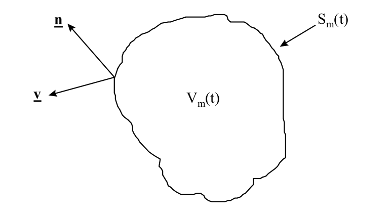
Consider a material volume $V_{m}(t)$ with surface area $S_{m}(t)$ . The unit normal to the surface is denoted by $\underline{\textbf{n}}$ and the surface velocity is denoted by $\underline{\textbf{v}}$ . But in our calculation $\underline{\textbf{n}}\Leftrightarrow\hat{\textbf{n}}$ and $\underline{\textbf{v}}\Leftrightarrow\textbf{U}$ . Within this control volume is a property of the continuum $\psi$ that is of interest. We would like to determine how $\psi$ changes with time. The total amount of $\psi$ present in the volume $V_{m}(t)$ can be expressed as:

\textbf{F}(t)=\int_{V_{m}(t)}\psi(\textbf{x},t)dV

(2.1)

The time rate of change if the fluid property is defined as:

\frac{d\textbf{F}}{dt}=\frac{d}{dt}\int_{V_{m}(t)}\psi(\textbf{x},t)dV

(2.2)

Since integration limit $V_{m}(t)$ is function of time so we can not take the derivative inside the integration directly. In order to overcome this problem we transform the volume, and material property from a spatial representation to a reference/material representation. Recall that any differential volume element at time t is

dV=JdV_{0}

where $dV_{0}$ is differential volume at t = 0 and Jacobian J is defined as

J=detF=\begin{bmatrix}\vspace{2mm}\frac{\partial x_{1}}{\partial X_{1}}&\frac{\partial x_{2}}{\partial X_{1}}&\frac{\partial x_{3}}{\partial X_{1}}\\ \vspace{2mm}\par\frac{\partial x_{1}}{\partial X_{2}}&\frac{\partial x_{2}}{\partial X_{2}}&\frac{\partial x_{3}}{\partial X_{2}}\\ \frac{\partial x_{1}}{\partial X_{3}}&\frac{\partial x_{2}}{\partial X_{3}}&\frac{\partial x_{3}}{\partial X_{3}}\end{bmatrix}

(2.3)

Given $\textbf{x}=\Phi(\textbf{X},t)$ also $\Psi(\textbf{x},t)$ can be expressed in terms of material coordinates by employing the results is

\Psi(\textbf{x},t)=\Psi({\Phi(\textbf{x},t)},t)=\Psi(\textbf{X},t)

Therefore we can express the integral in equation 2.2 in terms of the material coordinates:

\frac{d\textbf{F}}{dt}=\int_{V_{0}}\frac{d}{dt}\left[\Psi(\textbf{X},t)J\right]dV_{0}

\Rightarrow\frac{d\textbf{F}}{dt}=\int_{V_{0}}\left[\frac{d\Psi(\textbf{X},t)}{dt}J+\Psi(\textbf{X},t)\frac{dJ}{dt}\right]dV_{0}

\Rightarrow\frac{d\textbf{F}}{dt}=\int_{V_{0}}\left[\left(\frac{\partial\Psi(\textbf{X},t)}{\partial t}+(\textbf{U}\cdotp\nabla)\Psi\right)J+\Psi(\textbf{X},t)\frac{dJ}{dt}\right]dV_{0}

(2.4)

Where U is the velocity of control volume Now we recall J, from equation 2.3 we can say the J is function of $\frac{\partial\textbf{x}}{\partial\textbf{X}}$ i.e.

J=J\left(\frac{\partial\textbf{x}}{\partial\textbf{X}}\right)

\Rightarrow dJ=\frac{\partial J}{\partial\left(\frac{\partial\textbf{x}}{\partial\textbf{X}}\right)}d(\frac{\partial\textbf{x}}{\partial\textbf{X}})

\Rightarrow\frac{dJ}{dt}=\frac{\partial J}{\partial\left(\frac{\partial\textbf{x}}{\partial\textbf{X}}\right)}\frac{d}{dt}\left(\frac{\partial\textbf{x}}{\partial\textbf{X}}\right)

\Rightarrow\frac{dJ}{dt}=\frac{\partial J}{\partial\left(\frac{\partial\textbf{x}}{\partial\textbf{X}}\right)}\frac{\partial}{\partial X}\left(\frac{d\textbf{x}}{dt}\right)

\Rightarrow\frac{dJ}{dt}=J\left(\nabla\cdot\textbf{U}\right)

(2.5)

Now putting the value of $\frac{dJ}{dt}$ in equation 2.5 we get,

\frac{d\textbf{F}}{dt}=\int_{V_{0}}\left[\frac{\partial\Psi(\textbf{X},t)}{\partial t}+(\textbf{U}\cdotp\nabla)\Psi+\Psi(\textbf{X},t)\left(\nabla\cdot\textbf{U}\right)\right]JdV_{0}

\Rightarrow\frac{d\textbf{F}}{dt}=\int_{V_{m}(t)}\left[\frac{\partial\Psi}{\partial t}+\nabla\cdot\left(\textbf{U}\Psi\right)\right]dV_{m}

\Rightarrow\frac{d}{dt}\int_{V_{m}(t)}\Psi(\textbf{x},t)dV_{m}=\int_{V_{m}(t)}\left[\frac{\partial\Psi}{\partial t}+\nabla\cdot\left(\textbf{U}\Psi\right)\right]dV_{m}

(2.6)

This is known as Reynold’s Transport Theorem.[6] Now applying Gauss’s Divergence Theorem in $2^{nd}$ of the integral for the surface area $S_{m}(t)$ of the control volume of volume $V_{m}(t)$ we get

\frac{d\textbf{F}}{dt}=\int_{V_{m}(t)}\frac{\partial\Psi}{\partial t}dV_{m}+\int_{S_{m}(t)}\Psi\textbf{U}\cdot\hat{\textbf{n}}dS_{m}

\frac{d}{dt}\int_{V_{m}(t)}\Psi\left(\textbf{x},t\right)dV_{m}=\int_{V_{m}(t)}\frac{\partial\Psi}{\partial t}dV_{m}+\int_{S_{m}(t)}\Psi\textbf{U}\cdot\hat{\textbf{n}}dS_{m}

(2.7)

Rate of change at Net flow of $\Psi$ . a point volume across the surface $S_{m}(t)$

This is another form of RTT which is known as $\textbf{General Transport Theorem}.$

3 Conservation of Mass

Conservation of mass The constancy of mass is inherent in the definition of a control mass system and therefore we can write

\left(\frac{dm}{dt}\right)_{CMS}=0

(3.1)

The total mass of the the control volume can be defined as

m=\int_{V_{m(t)}}\rho dV_{m}

To develop the analytical statement for the conservation of mass of a control volume, by using equation 2.6 we get,

\frac{d\textbf{m}}{dt}=\int_{V_{m}(t)}\left[\frac{\partial\rho}{\partial t}+\nabla\cdot\left(\textbf{U}\rho\right)\right]dV_{m}

\Rightarrow\int_{V_{m}(t)}\left[\frac{\partial\rho}{\partial t}+\nabla\cdot\left(\textbf{U}\rho\right)\right]dV_{m}=0

\frac{\partial\rho}{\partial t}+\nabla\cdot\left(\textbf{U}\rho\right)=0

(3.2)

This known as mass conservation equation also known as differential form of continuity equation.

4 ConservatioFconsern of Momentum

Conservation of Momentum or Momentum Theorem The principle of conservation of momentum as applied to a control volume is usually referred to as the momentum theorem.The first step in deriving the analytical statement of linear momentum theorem is to write the equation 2.7 for the property $\Psi$ as the linear-momentum $m\textbf{u}$ and the velocity u along x-direction . Then it becomes

\frac{d}{dt}\int_{V_{m}(t)}\rho udV_{m}=\int_{V_{m}(t)}\left[\frac{\partial}{\partial t}\left(\rho u\right)+\nabla\cdot\left(\rho u\textbf{U}\right)\right]dV_{m}

(4.1)

\Rightarrow\frac{d}{dt}\int_{V_{m}(t)}\rho udV_{m}=\int_{V_{m}(t)}\left[\frac{\partial}{\partial t}\left(\rho u\right)+\nabla\cdot\left(\rho u\textbf{U}\right)\right]dV_{m}

=\int_{V_{m}(t)}u\left[\frac{\partial\rho}{\partial t}+\nabla\cdot\rho\textbf{U}\right]+\left[\rho\frac{\partial u}{\partial t}+\rho\textbf{U}\cdot\nabla u\right]dV_{m}

The last term of $1^{st}$ term of the integral and first term of $2^{nd}$ term of the integral create shows the equation of mass conservation which gives zero. so that

\int_{V_{m}(t)}\left[\rho\frac{\partial\rho}{\partial t}+\rho\textbf{U}\cdot\nabla u\right]dV_{m}=\int_{V_{m}(t)}\rho\frac{du}{dt}dV_{m}

(4.2)

From equation 4.1 and 4.2 we get (similar equations can be derived for v and w as well)

\int_{V_{m}(t)}\rho\frac{d\textbf{U}}{dt}dV_{m}=\int_{V_{m}(t)}\textbf{F}_{B}dV_{m}+\int_{S_{m}(t)}\textbf{F}_{S}dS_{m}

(4.3)

We begin by noting that $\textbf{F}_{S}$ be a vector that there must be a matrix say T such that

\textbf{F}_{s}=\textbf{T}\cdot\hat{\textbf{n}}

Notice that the ”dot” notation for the matrix-vector product is used to emphasize that each component of $\textbf{F}_{S}$ is the (vector) dot product of the corresponding row of T with the unit column vector $\hat{\textbf{n}}$ . So we get

\int_{V_{m}(t)}\rho\frac{d\textbf{U}}{dt}dV_{m}=\int_{V_{m}(t)}\textbf{F}_{B}dV_{m}+\int_{S_{m}(t)}\textbf{T}\cdot\hat{\textbf{n}}dS_{m}

By using Gauss Divergence Theorem for the last term of RHS and recalling $V_{m}(t)$ as arbitrary fluid element, we get

\rho\frac{d\textbf{U}}{dt}-\textbf{F}_{B}-\nabla\cdot\textbf{T}=0

(4.4)

This provides a fundamental and very general momentum balance that is valid at all points of any fluid flow (following the continuum hypothesis). T is reason of surface force. Now we are not going to more expression of T. Now writing the final form of T

\textbf{T}=\begin{bmatrix}\vspace{2 mm}-P+\tau_{xx}&\tau_{xy}&\tau_{xz}\\ \vspace{2 mm}\tau_{yx}&-P+\tau_{yy}&\tau_{yz}\\ \tau_{zx}&\tau_{zy}&-P+\tau_{zz}\end{bmatrix}

(4.5)

\Rightarrow\textbf{T}=-P\textbf{I}+\tau

In this equation I is the identity matrix, and $\tau$ is often termed the viscous stress tensor. The expression will be clear from the picture

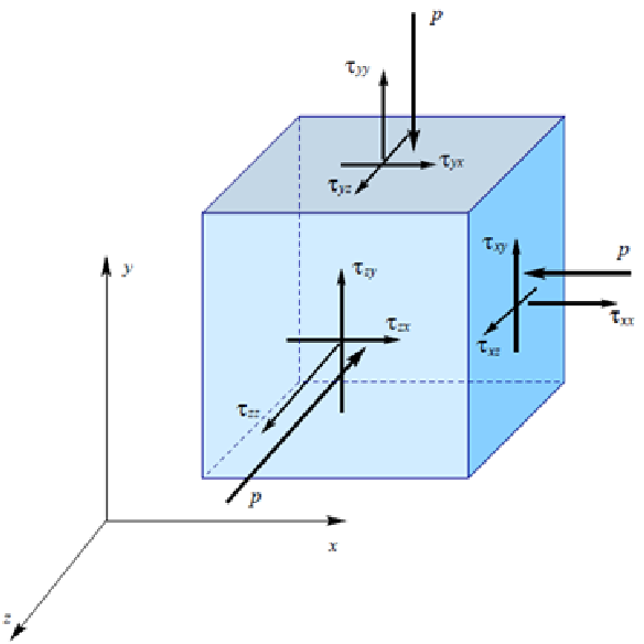
From Newton’s law of viscosity we can express the components of shear stress

\tau_{xy}=\mu\left(\frac{\partial u}{\partial y}+\frac{\partial v}{\partial x}\right)

Putting this value in equation 4.4 we get(in component form)

\begin{split}\rho\frac{du}{dt}=-P_{x}+\mu\left(u_{xx}+u_{yy}+u_{zz}\right)+F_{B_{,x}}\\ \rho\frac{dv}{dt}=-P_{y}+\mu\left(v_{xx}+v_{yy}+v_{zz}\right)+F_{B_{,y}}\\ \rho\frac{dv}{dt}=-P_{z}+\mu\left(w_{xx}+w_{yy}+w_{zz}\right)+F_{B_{,z}}\end{split}

(4.6)

Now divide these equations by $\rho$ on both side and express them as

\begin{split}\frac{\partial u}{\partial t}+u\frac{\partial u}{\partial x}+v\frac{\partial u}{\partial y}+w\frac{\partial u}{\partial z}=\frac{\partial P}{\partial x}+\nu\triangle u+\frac{1}{\rho}+F_{B_{,x}}\\ \frac{\partial v}{\partial t}+u\frac{\partial v}{\partial x}+v\frac{\partial v}{\partial y}+w\frac{\partial v}{\partial z}=\frac{\partial P}{\partial y}+\nu\triangle v+\frac{1}{\rho}+F_{B_{,y}}\\ \frac{\partial w}{\partial t}+u\frac{\partial w}{\partial x}+v\frac{\partial w}{\partial y}+w\frac{\partial w}{\partial z}=\frac{\partial P}{\partial z}+\nu\triangle w+\frac{1}{\rho}+F_{B_{,z}}\end{split}

(4.7)

Here, $\nu$ is kinematic viscosity, the ratio of viscosity $\mu$ to density $\rho$ and $\triangle$ is the second-order partial differential operator (given here in Cartesian coordinates)

\triangle=\frac{\partial^{2}}{\partial x^{2}}+\frac{\partial^{2}}{\partial y^{2}}+\frac{\partial^{2}}{\partial z^{2}}

This is known as momentum conservation equation but well known as Nevier-Stokes Equation. and they provide a pointwise description of essentially any time-dependent incompressible fluid flow.

5 Energy Conservation

Let E be the total energy of the fluid, sum of its kinetic energy and internal energy:

E=E_{k}+E_{int}=\frac{1}{2}\int_{V_{m}(t)}\rho\textbf{u}^{2}dV_{m}+\int_{V_{m}(t)}\rho\epsilon dV_{m}

Principle of energy conservation: “the variation in time of the total energy of a portion of fluid is equal to the work done per unit time over the system by the stresses (internal forces) and the external forces”. Apply E in $\bf{RTT}$ equation 2.6, we get

\frac{dE}{dt}=\frac{d}{dt}\int_{V_{m}(t)}\left(\frac{1}{2}\rho\textbf{u}^{2}+\rho\epsilon\right)dV_{m}=\int_{V_{m}(t)}\left[\frac{\partial}{\partial t}\left(\frac{1}{2}\rho\textbf{u}^{2}+\rho\epsilon\right)+\nabla\cdot\left(\frac{1}{2}\textbf{u}\rho\textbf{u}^{2}+\textbf{u}\rho\epsilon\right)\right]dV_{m}

(5.1)

Here, $\frac{\partial}{\partial t}\left(\frac{1}{2}\rho u^{2}\right)=\rho u_{i}\frac{\partial u_{i}}{\partial t}$ and substituting in equation 4.7, we get

\frac{\partial u_{i}}{\partial t}=-u_{k}\frac{\partial u_{i}}{\partial x_{k}}-\frac{1}{\rho}\frac{\partial P}{\partial x_{i}}+u_{i}\frac{\partial\sigma_{ik}}{\partial x_{k}}

The result is

\frac{\partial}{\partial t}\left(\frac{1}{2}\rho\textbf{u}^{2}\right)=-\rho\textbf{u}\cdot\left(\textbf{u}\cdot\nabla\right)\textbf{u}-\textbf{u}\cdot\nabla P+u_{i}\frac{\partial\sigma_{ik}}{\partial x_{k}}

\Rightarrow\frac{\partial}{\partial t}\left(\frac{1}{2}\rho\textbf{u}^{2}\right)=-\rho\left(\textbf{u}\cdot\nabla\right)\left(\frac{u^{2}}{2}+\frac{P}{\rho}\right)+\nabla(\textbf{u}\cdot\sigma)-\sigma_{ik}\frac{\partial u_{i}}{\partial x_{k}}

Here $\textbf{u}\cdot\sigma$ denotes the vector whose components are $u_{i}\sigma_{ik}$ . Since $\nabla\cdot\textbf{u}=0$ for an incompressible fluid, we can write the first term on the right as a divergence:

\frac{\partial}{\partial t}\left(\frac{1}{2}\rho\textbf{u}^{2}\right)=-\nabla\cdot\left[\rho\textbf{u}\left(\frac{1}{2}\textbf{u}^{2}+\frac{P}{\rho}\right)-\textbf{u}\cdot\sigma\right]-\sigma_{ik}\frac{\partial u_{i}}{\partial x_{k}}

(5.2)

$\Downarrow$ $\Downarrow$ $\Downarrow$

Energy Flux Energy Flux Energy Flux

due to actual due to Friction due to momentum

mass transfer change

Now from equation 5.1, we get

\int_{V_{m}(t)}\left[\frac{\partial}{\partial t}\left(\frac{1}{2}\rho\textbf{u}^{2}+\rho\epsilon\right)+\nabla\cdot\left(\left(\frac{1}{2}\rho\textbf{u}^{2}+\rho\epsilon+P\right)\textbf{u}-\textbf{u}\cdot\sigma\right)\right]dV_{m}=-\int_{V_{m}(t)}\sigma_{ik}\frac{\partial u_{i}}{\partial x_{k}}

(5.3)

This is known as Energy conservation equation.[2]

6 Euler Equation:

The purpose of this note derivation of Euler’s equation for fluid flow on the basis of conservation of mass, conservation of momentum and Newton’s laws.

To set the stage, consider the example shown in figure 4. The top half is a snapshot of the fluid at some initial time $t_{0}$ and the bottom half is a snapshot at some slightly later time $t_{1}$ . One parcel of fluid has been marked with blue dye, and another parcel has been marked with red dye. The rectangle represents an imaginary box, also called the “Control Volume” we will be particularly interested in what is happening within this box.

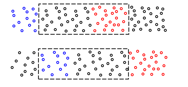
There are some qualitative observations that we can make immediately:

$\ast$

The fluid is flowing left-to-right.
$\ast$

The density depends on position: The red parcel is denser than the blue parcel.
$\ast$

The density depends on time: The density in the control volume decreases as time passes from $t_{0}$ to $t_{1}$ .
$\ast$

The velocity depends on position: during the time interval in question, the right edge of the blue parcel moves a relatively short distance, while the right edge of the red parcel moves a relatively long distance.
$\ast$

The total number of red particles does not change, and the total number of blue particles does not change. (Some particles that flow out of the frame of the diagram are not accounted for, but all particles -red, blue, or black-that affect the control volume are accounted for.

In our calculations, we consider the following assumptions

‡

The fluid is ideal gas.
‡

There is no viscous force i.e $\mu=0$
‡

There is no external force.
‡

Fluid flow is one dimensional.

Now applying this assumption on equation 3.2

\frac{\partial\rho}{\partial t}+\nabla\cdot\left(\rho\textbf{u}\right)=0

\Rightarrow\frac{\partial\rho}{\partial t}+\frac{\partial\left(\rho u\right)}{\partial x}=0

(6.1)

This is Mass Conservation equation for ideal gas.

$\star$ Momentum Conservation: In some volume of fluid with surface $S_{m}(t)$ the total force acting on the volume $V_{m}(t)$ is $-\int_{S_{m}(t)}PdS_{m}=-\int_{V_{m}(t)}\nabla PdV_{m}$ where P is the pressure. Applying force on unit volume $\rho\frac{d\textbf{u}}{dt}$ (Newton’s $2^{nd}$ Law). Then we may be written as

\rho\frac{d\textbf{u}}{dt}=-\nabla P

By using RTT equation 2.6, we get

\frac{\partial(\rho\textbf{u})}{\partial t}+\nabla\cdot\left[\textbf{u}\otimes\left(\rho\textbf{u}\right)\right]=0

\Rightarrow\frac{\partial\left(\rho u_{j}\right)}{\partial t}+\sum_{i=1}^{3}\frac{\partial\left(\rho u_{i}u_{j}\right)}{\partial x_{i}}+\frac{\partial P}{\partial x_{j}}=0

But for one dimensional case $i=j=1$ , then

\frac{\partial\left(\rho u\right)}{\partial t}+\frac{\partial\left(\rho u^{2}+P\right)}{\partial x}=0

(6.2)

This is Momentum conservation and now applying the assumption on energy equation 5.3:

\int_{V_{m}(t)}\left[\frac{\partial\left(\rho\textbf{u}^{2}+\rho\epsilon\right)}{\partial t}+\nabla\cdot\left(\left(\frac{1}{2}\rho\textbf{u}^{2}+\rho\epsilon+P\right)\textbf{u}\right)\right]dV_{m}=0

recalling arbitrary value of elementary volume and applying one dimensional case

\Rightarrow\frac{\partial\left(\rho u^{2}+\rho\epsilon\right)}{\partial t}+\frac{\partial}{\partial x}\left[\left(\frac{1}{2}\rho u^{2}+\rho\epsilon+P\right)u\right]=0

Total energy of ideal gas $e=\frac{1}{2}\rho u^{2}+\rho\epsilon$ , so

\frac{\partial e}{\partial t}+\frac{\partial}{\partial x}\left[u\left(e+P\right)\right]=0

(6.3)

This is known as Energy Conservation equation for ideal gas.

7 Finite Volume Method

The finite-volume method[5] is a method for representing and evaluating partial differential equations in the form of algebraic equations. In this method values are calculated from at discrete places at meshed geometry. ”Finite Volume” refers small volume surroundings about mesh grid point. The evaluated terms are Fluxes at the surface of referred volume. Because the flux entering a given volume is identical to that leaving the adjacent volume, these methods are conservative. This method is used in many CFD packages.

Let us consider a 1 Dimensional Hyperbolic Equation can be defined by partial differential equation

\frac{\partial\rho}{\partial t}+\frac{\partial\Psi}{\partial x}=0,\hskip 19.91692ptt\geq 0

(7.1)

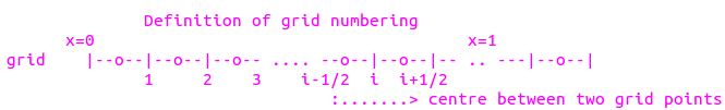
Where, $\rho=\rho(x,t)$ represents the state variable and $\Psi=\Psi(x,t)$ represents the flux or flow of $\rho$ .Conventionally, positive $\Psi$ indicates flow from left to right and negative $\Psi$ indicates flow from right to left.If we assume that equation (7.1) represents a flowing medium of constant area, we can sub-divide the spatial domain x, into finite volumes or cells with cell center index i. For a particular cell ’i’ we can define the volume average value of $\rho_{i}(t)=\rho(x,t)$ at time t = $t_{1}$ and $x\in[x_{i-1/2},x_{i+1/2}]$ . Just look at the figure

Now average value equation is

\bar{\rho_{i}}(t_{1})=\frac{1}{x_{i+1/2}-x_{i-1/2}}\int_{x_{i-1/2}}^{x_{i+1/2}}\rho(x,t_{1})dx

(7.2)

At time $t=t_{2}$ , the average value equation is

\bar{\rho_{i}}(t_{2})=\frac{1}{x_{i+1/2}-x_{i-1/2}}\int_{x_{i-1/2}}^{x_{i+1/2}}\rho(x,t_{2})dx

(7.3)

Where, $x_{i-1/2}$ and $x_{i+1/2}$ represent locations of the upstream and downstream faces or edges respectively of the $i^{th}$ cell. Now integrating equation(7.1) with respect to time, we have:

\rho_{i}(t_{2})=\rho_{i}(t_{1})-\int_{t_{1}}^{t_{2}}\Psi_{x}(x,t)dt

(7.4)

where $\Psi_{x}=\frac{\partial\Psi}{\partial x}$ , To obtain the volume average $\rho(x,t)$ at time $t=t_{2}$ we integrate $\rho(x,t_{2})$ over the cell volume $[x_{i-1/2},x_{i+1/2}]$ after then we divide the result by $\triangle x_{i}=x_{i+1/2}-x_{i-1/2}$ , implies that

\bar{\rho_{i}}(t_{2})=\frac{1}{\triangle x_{i}}\int_{x_{i-1/2}}^{x_{i+1/2}}\textbf{[}\rho(x,t_{1})-\int_{t_{1}}^{t_{2}}\Psi_{x}(t,x)\textbf{]}dx

(7.5)

we can assume that $\Psi$ is well behaved and flow is normal to the surface area, even for 1 D case $\Psi_{x}\sim\bigtriangledown\Psi$ , so we can apply gauss divergence theorem in equation(7.5) over the x region $[x_{i-1/2},x_{i+1/2}]$ even x and t are independent to each other i.e. we can interchange the integration of dx and dt, now we have:

\bar{\rho_{i}}(t_{2})=\frac{1}{\triangle x_{i}}\int_{x_{i-1/2}}^{x_{i+1/2}}\rho(x,t_{1})dx-\frac{1}{\triangle x_{i}}\int_{t_{1}}^{t_{2}}\textbf{[}\int_{x_{i-1/2}}^{x_{i+1/2}}\Psi_{x}(t,x)dx\textbf{]}dt

(7.6)

\bar{\rho_{i}}(t_{2})=\bar{\rho}(x,t_{1})-\frac{1}{\triangle x_{i}}\int_{t_{1}}^{t_{2}}\textbf{[}\Psi_{x_{i+1/2}}-\Psi_{x_{i-1/2}}\textbf{]}dt

(7.7)

We can therefore derive semi discrete numerical method with cell center index i and edges at $i\pm 1/2$ :

\frac{d\bar{\rho_{i}}}{dt}=\frac{1}{\triangle x_{i}}{\textbf{[}{\Psi_{i+1/2}-\Psi_{i-1/2}}\textbf{]}}

(7.8)

where values for the edge fluxes, $\Psi_{i+1/2},\Psi_{i-1/2}$ can be reconstructed by interpolation or extrapolation of the cell averages. Equation (7.8) is exact for the volume averages; i.e., no approximations have been made during its derivation.

8 Roe Scheme Method

Roe Scheme Method[1] is a method to solve fluid conservation laws which are based on exploiting the information obtained by considering a sequence of Riemann Problem. It is argued that in existing schemes much of this information is degraded, and that only certain features of the exact solution are worth striving.

we consider the initial value problem for a hyperbolic system of conservation laws, such that

\textbf{u}_{t}+\textbf{F}_{x}=0

(8.1)

where, $\textbf{u}=\textbf{u}(x,t)$ and

\textbf{u}(x,0)=\textbf{u}_{0}(x)

(8.2)

Where, F is some vector-valued function of u, such that the Jacobian matrix $A=\frac{\partial\textbf{F}}{\partial\textbf{u}}$ has only real eigenvalues, by using the discrete representation $x_{i}=x_{0}+i\triangle x$ and $t_{n}=t_{0}+n\triangle t$ and consider $\textbf{u}_{i}^{n}$ is some approximation of $\textbf{u}(x_{i},t_{n})$ but a multitude of strategies are required to obtain the numerical result which is unclear, so we recall Riemann Problem and condition are:

\textbf{u}(x,0)\equiv\textbf{u}_{L}\hskip 19.91692pt(x<0);\hskip 28.45274pt\textbf{u}(x,0)=\textbf{u}_{R}\hskip 19.91692pt(x>0)

(8.3)

Now we can solve exactly equation 8.1 by using this initial condition and corresponding system equation where equation(8.1) will be converted to $\textbf{u}_{t}+A\textbf{u}_{x}=0$ , which is our exact solution, but now we try to solve the equation(8.1) by boundary value and which gives us the approximate solution.

we consider the approximate solutions

\textbf{u}_{t}+\tilde{A}\textbf{u}_{x}=0

(8.4)

where, $\tilde{A}=\tilde{A}(\textbf{u}_{L},\textbf{u}_{R})$ which satisfy the properties:

1.

It constitutes a linear mapping from the vector space u to the vector space F
2.

As $\textbf{u}_{L}\textbf{u}_{R}\rightarrow\textbf{u}$ , $\bar{A}(\textbf{u}_{l},\textbf{u}_{R})\rightarrow A(\textbf{u})$ , where $A=\frac{\partial\textbf{F}}{\partial\textbf{u}}$
3.

For any $\textbf{u}_{L}$ , $\textbf{u}_{R}$ , $\tilde{A}(\textbf{u}_{L},\textbf{u}_{R})\times(\textbf{u}_{L}-\textbf{u}_{R})=\textbf{F}_{L}-\textbf{F}_{R}$
4.

The eigenvectors of $\tilde{A}$ are linearly independent.

8.1 Parameter Vector:

In this section we will use experience in analytic geometry that a plane curve y(x) may in some cases be much more easily described by a parametric form y = y(t) and x = x(t). we may therefore expect that a multidimensional manifold such as $\textbf{F}(\textbf{u})$ may sometimes be more amenable if represented as $\textbf{F}=\textbf{F}(\textbf{w})$ , $\textbf{u}=\textbf{u}(\textbf{w})$ where w as a parameter vector. Now we exhibit parameter vector for the Euler Equations, which we write as

\textbf{u}_{t}+\textbf{F}_{x}=0,

(8.5)

where

\boxed{\textbf{u}=\begin{bmatrix}\rho\\ \rho u\\ e\\ \end{bmatrix},\hskip 42.67912pt\textbf{F}=\begin{bmatrix}\rho u\\ P+\rho u^{2}\\ u(P+e)\\ \end{bmatrix}}

(8.6)

in which $\rho$ = density, P = static pressure, u = velocity in Cartesian coordinate x, and e is total energy per unit volume. For ideal gas equation :

P=\rho RT=\rho(C_{P}-C_{V})T=\rho(\gamma-1)C_{V}T=\rho(\gamma-1)\bar{e}

(8.7)

$\bar{e}$ = internal energy per unit mass, so internal energy per unit volume $\rho\bar{}\bar{e}=P/(\gamma-1)$ so Total energy = Kinetic energy + Thermal energy i.e.

\boxed{e=\frac{1}{2}\rho u^{2}+P/(\gamma-1)}

(8.8)

Now we take the parameter vector as like $\textbf{w}=\rho^{\frac{1}{2}}(1,u,h)^{T}$ where h = enthalpy is defined as

\rho h=e+P=\frac{1}{2}\rho u^{2}+\frac{P}{(\gamma-1)}+P

(8.9)

\boxed{h-\frac{u^{2}}{2}=\frac{\gamma P}{(\gamma-1)\rho}}

(8.10)

\boxed{(\gamma-1)(h-\frac{u^{2}}{2})=\frac{\gamma P}{\rho}}

(8.11)

Now from the expression of w and from equation 8.6, we have

u_{1}=w_{1}^{2},\hskip 19.91692ptu_{2}=w_{1}w_{2},\hskip 19.91692ptu_{3}=\frac{w_{1}w_{3}}{\gamma}+\frac{\gamma-1}{2\gamma}w_{2}^{2}

(8.12)

and

F_{1}=w_{1}w_{2}

F_{2}=P+\rho u^{2}

=\frac{\gamma-1}{\gamma}(\rho h-\frac{\rho u^{2}}{2})+\rho u^{2}

=\frac{\gamma-1}{\gamma}\rho h+\frac{\gamma+1}{2\gamma}\rho u^{2}

=\frac{\gamma-1}{\gamma}w_{1}w_{3}+\frac{\gamma+1}{2\gamma}w_{2}^{2}

F_{3}=u(P+e)=u\rho h=w_{2}w_{3}

(8.13)

8.2 Eigenvalues and Eigenvectors for Euler Equation

It is now very easy to represent any jump in space u,F in terms of its image in the space w. For example, given any pair of states $(\textbf{u}_{L},\textbf{u}_{R})$ and their images $(\textbf{w}_{L},\textbf{w}_{r})$ we can write

\left(\textbf{u}_{L}-\textbf{u}_{R}\right)\equiv\tilde{\textbf{B}}\left(\textbf{w}_{L}-\textbf{w}_{R}\right)

(8.14)

and

\left(\textbf{F}_{L}-\textbf{F}_{R}\right)\equiv\tilde{\textbf{C}}\left(\textbf{w}_{L}-\textbf{w}_{R}\right)

(8.15)

where $\tilde{\textbf{B}}$ , $\tilde{\textbf{C}}$ are $3\times 3$ matrix, now $\tilde{\textbf{B}}$ can be evaluated by the process:

u_{L1}-u_{R1})=\tilde{B}_{11}\left(w_{L1}-w_{R1}\right)+\tilde{B}_{12}\left(w_{L2}-w_{R2}\right)+\tilde{B}_{13}\left(w_{L3}-w_{R3}\right)

(w_{L1}^{2}-u_{R1}^{2})=\tilde{B}_{11}(w_{L1}-w_{R1})+\tilde{B}_{12}(w_{L2}-w_{R2})+\tilde{B}_{13}(w_{L3}-w_{R3})

So there is only one solution for $\tilde{B}_{11}=\frac{w_{L1}^{2}-w_{L2}^{2}}{w_{L1}-w_{R1}}=\bar{w}_{1}$ where $\bar{w}_{1}=\frac{1}{2}(w_{L1}+w_{R1})$ and $\tilde{B}_{12}$ , $\tilde{B}_{13}$ are zero. Similarly we evaluate another component of $\tilde{\textbf{B}}$

u_{L2}-u_{R2}=\tilde{B}_{21}(w_{L1}-w_{R1})+\tilde{B}_{22}(w_{L2}-w_{R2})+\tilde{B}_{23}(w_{L3}-w_{R3})

\Rightarrow w_{L1}w_{L2}-w_{R1}w_{R2}=\tilde{B}_{21}(w_{L1}-w_{R1})+\tilde{B}_{22}(w_{L2}-w_{R2})+\tilde{B}_{23}(w_{L3}-w_{R3})

Here $\tilde{B}_{23}=0$ , because LHS have no term of $w_{L3}$ or $w_{R3}$ . Now we try to solve the reduced equation. There are two solution but we have to choose the solution which containing $w_{L}$ and $w_{R}$ both. So the reduced equation is

w_{L1}w_{L2}-w_{R1}w_{R2}=\tilde{B}_{21}(w_{L1}-w_{R1})+\tilde{B}_{22}(w_{L2}-w_{R2})

Where $\tilde{B}_{21}=\frac{1}{2}(w_{L2}+w_{R2})=\bar{w}_{2}$ and $\tilde{B}_{22}=$ $\frac{1}{2}(w_{L1}+w_{R2})=\bar{w}_{1}$ , similarly solving the third equation we have the matrix $\tilde{\textbf{B}}$ as

\tilde{\textbf{B}}=\begin{bmatrix}\vspace{3mm}2\bar{w}_{1}&0&0\\ \vspace{3mm}\bar{w}_{2}&\bar{w}_{1}&0\\ \frac{\bar{w_{3}}}{\gamma}&\frac{\gamma-1}{\gamma}\bar{w_{2}}&\frac{\bar{w}_{1}}{\gamma}\\ \end{bmatrix}

(8.16)

and by using equivalent method

\tilde{\textbf{C}}=\begin{bmatrix}\vspace{3mm}\bar{w}_{2}&\bar{w}_{1}&0\\ \vspace{3mm}\frac{\gamma-1}{\gamma}\bar{w}_{3}&\frac{\gamma+1}{\gamma}\bar{w}_{2}&\frac{\gamma-1}{\gamma}\bar{w}_{1}\\ 0&\bar{w}_{3}&\bar{w}_{2}\end{bmatrix}

(8.17)

Obviously these very simple formulas are closely related to the homogeneous property of the Euler equations. We will wish to construct the eigenvalues and the eigenvectors of some matrix $\tilde{A}$ which maps $\triangle\textbf{u}$ and $\triangle\textbf{F}$ with property u. Evidently we may choose $\tilde{A}=(\tilde{\textbf{C}})(\tilde{\textbf{B}})^{-1}$ . To find the find the eigenvalues and eigenvectors we simplify the matrix $\tilde{\textbf{B}}$ and $\tilde{\textbf{C}}$ divide by $\bar{w}_{1}$ without loss of property.

\boxed{\frac{\bar{w}_{2}}{\bar{w}_{1}}=\frac{\rho_{L}^{\frac{1}{2}}u_{L}+\rho_{R}^{\frac{1}{2}}u_{R}}{\rho_{L}^{\frac{1}{2}}+\rho_{R}^{\frac{1}{2}}}=\bar{u}}

(8.18)

\boxed{\frac{\bar{w}_{3}}{\bar{w}_{1}}=\frac{\rho_{L}^{\frac{1}{2}}h_{L}+\rho_{R}^{\frac{1}{2}}h_{R}}{\rho_{L}^{\frac{1}{2}}+\rho_{R}^{\frac{1}{2}}}=\bar{h}}

(8.19)

we use Python code to determine the eigenvalues and eigenvector of new $\tilde{\textbf{B}}$ and $\tilde{\textbf{C}}$ :

⬇

#!/usr/bin/env python

# -*- coding: utf-8 -*-

from sympy import S, pprint,symbols, simplify

from sympy.matrices import *

from sympy.interactive.printing import init_printing

init_printing = init_printing(use_unicode=False,

wrap_line=False,no_global=True)

u, h, gamma = symbols(’u h gamma’)

gammaA = ((gamma-1)/gamma)

gammaB = ((gamma+1)/gamma)

C = Matrix([[u, 1, 0], [gammaA*h, gammaB*u, gammaA], [0, h, u]])

BP = Matrix([[2, 0, 0], [u, 1, 0], [h/gamma, gammaA*u, 1/gamma]])

B = Inverse(BP)

A = C*B

lam = A.eigenvals()

vec = A.eigenvects()

Corresponding results are :

\tilde{A}=\begin{bmatrix}\vspace{3mm}0&1&0\\ \vspace{3mm}\frac{\bar{u}^{2}}{2\gamma}(\gamma^{2}-3\gamma)&\frac{-\bar{u}(\gamma^{2}-3\gamma)}{\gamma}&\gamma-1\\ \bar{u}(\bar{a}^{2}-\gamma\bar{h})&-2\bar{a}^{2}-\bar{h}+2\gamma\bar{h}&\gamma\bar{u}\end{bmatrix}

(8.20)

\boxed{\lambda_{1}=\bar{u},\hskip 28.45274pt\lambda_{2}=\bar{a},\hskip 28.45274pt\lambda_{3}=\bar{u}+\bar{a}}

(8.21)

\boxed{e_{1}=\begin{bmatrix}\vspace{3 mm}1\\ \vspace{3 mm}\bar{u}-\bar{a}\\ \bar{h}-\bar{u}\bar{a}\\ \end{bmatrix},\hskip 14.22636pte_{2}=\begin{bmatrix}\vspace{3 mm}1\\ \vspace{3 mm}\bar{u}\\ \frac{\bar{u}^{2}}{2}\end{bmatrix},\hskip 14.22636pte_{3}=\begin{bmatrix}\vspace{3 mm}1\\ \vspace{3 mm}\bar{u}+\bar{a}\\ \bar{h}+\bar{u}\bar{a}\\ \end{bmatrix}}

(8.22)

Here $\bar{a}^{2}=(\gamma-1)(\bar{h}-\bar{u}^{2}/2)=\frac{\gamma\bar{P}}{\bar{\rho}}$ (by using equation 8.11 ), $\lambda$ ’s are eigenvalues and $e_{i}$ are eigenvectors.

8.3 Approximate Riemann Solver

To complete the analysis we must show how to project an arbitrary $\triangle u$ onto the eigenvectors as basis i.e., we have to find coefficient $\alpha_{i}$ in

\triangle u=\sum_{i=1}^{3}\alpha_{i}e_{i}

(8.23)

A routine calculation yields

\triangle u_{1}=\alpha_{1}+\alpha_{2}+\alpha{3}

\triangle u_{2}=\alpha_{1}(\bar{u}-\bar{a})+\alpha_{2}\bar{u}+\alpha_{3}(\bar{u}+\bar{a})

\Rightarrow\triangle u_{2}=(\alpha_{1}+\alpha_{2}+\alpha{3})\bar{u}+(\alpha_{3}-\alpha_{1})\bar{a}

\Rightarrow\triangle u_{2}-\bar{u}\triangle u_{1}=(\alpha_{3}-\alpha_{1})\bar{a}

\triangle u_{3}=\alpha_{1}(\bar{h}-\bar{u}\bar{a})+\alpha_{2}\frac{\bar{u}^{2}}{2}+\alpha_{3}(\bar{h}+\bar{u}\bar{a})

\Rightarrow\triangle u_{3}=(\alpha_{3}-\alpha_{1})\bar{u}\bar{a}+\alpha_{2}\frac{\bar{u}^{2}}{2}+(\alpha_{1}+\alpha_{3})\bar{h}

\Rightarrow\triangle u_{3}=(\triangle u_{2}-\bar{u}\triangle u_{1})\bar{u}+\alpha_{2}\frac{\bar{u}^{2}}{2}+(\triangle u_{1}-\alpha_{2})\bar{h}

\Rightarrow\triangle u_{3}=(\bar{h}-\bar{u}^{2})\triangle u_{1}+\alpha_{2}\frac{u^{2}}{2}+\bar{u}\triangle u_{2}

\Rightarrow\frac{\bar{a}^{2}}{\gamma-1}\alpha{2}=(\bar{h}-\bar{u}^{2})\triangle u_{1}+u\triangle u_{2}-\triangle u_{3}

\Rightarrow\frac{a^{2}}{\gamma-1}\alpha{2}=(\frac{\bar{a}^{2}}{\gamma-1}-\frac{\bar{u}^{2}}{2})\triangle u_{1}+\bar{u}\triangle u_{2}-\triangle u_{3}

\Rightarrow\boxed{\alpha_{2}=(1-\frac{(\gamma-1)\bar{u}^{2}}{2\bar{a}^{2}})\triangle u_{1}+\frac{(\gamma-1)\bar{u}}{\bar{a}^{2}}\triangle u_{2}-\frac{\gamma-1}{\bar{a}^{2}}\triangle u_{3}}

(8.24)

Now from the $1^{st}$ equation :

\alpha_{1}+\alpha_{3}=\triangle u_{1}-\alpha_{2}

\Rightarrow\alpha_{1}+\alpha_{3}=\frac{(\gamma-1)\bar{u}^{2}}{2\bar{a}^{2}}\triangle u_{1}-\frac{(\gamma-1)\bar{u}}{\bar{a}^{2}}\triangle u_{2}+\frac{(\gamma-1)}{\bar{a}^{2}}\triangle u_{3}

and from $2^{nd}$ equation:

-\alpha_{1}+\alpha_{3}=\frac{1}{a}(\triangle u_{2}-u\triangle u_{1})

So we are able to solve $\alpha_{1}$ and $\alpha_{3}$ :

\boxed{\alpha_{1}=\frac{\bar{u}}{4\bar{a}}\left[2+\frac{(\gamma-1)\bar{u}}{\bar{a}}\right]\triangle u_{1}-\frac{1}{2\bar{a}}\left[1+\frac{(\gamma-1)\bar{u}}{\bar{a}}\right]\triangle u_{2}+\frac{\gamma-1}{2\bar{a}^{2}}\triangle u_{3}}

(8.25)

\boxed{\alpha_{3}=-\frac{\bar{u}}{4\bar{a}}\left[2+\frac{(\gamma-1)\bar{u}}{\bar{a}}\right]\triangle u_{1}+\frac{1}{2\bar{a}}\left[1-\frac{(\gamma-1)\bar{u}}{\bar{a}}\right]\triangle u_{2}+\frac{\gamma-1}{2\bar{a}^{2}}\triangle u_{3}}

(8.26)

Now we construct $\triangle F$ , which will construct by the eigenvalues and eigenvectors of $\tilde{A}$ which maps $\triangle u$ and $\triangle F$ and must be multiplied by $\alpha_{i}$ ’s because $\tilde{A}$ in image space w. So we have:

\triangle F=\sum_{i}\lambda_{i}\alpha_{i}e_{i}

Now we have have the information $F_{i}$ and $F_{i+1}$ on the mesh grid point so intermediate Flux is given by:

F_{i+1/2}=\frac{1}{2}(F_{i+1}+F_{i})-\frac{1}{2}\sum{\lambda_{i}\alpha_{i}e_{i}}

\Rightarrow F_{i+1/2}=\frac{1}{2}(F_{L}+F_{R})-\frac{1}{2}\sum{\lambda_{i}\alpha_{i}e_{i}}

(8.27)

8.4 Harten Sonic Entropy Fix

when, $\bar{u}=\bar{a}$ then $\lambda_{1}=\bar{u}-\bar{a}=0$ so

\Rightarrow F_{i+1/2}=\frac{1}{2}(F_{L}+F_{R})

This means that central discretization is used, without artificial viscosity so that there is a danger that entropy decreases, and that discontinuities are insufficiently smear out. The flow is not sonic , then we do not have central discretization , and there may be enough dissipation to prevent violation of the entropy condition. this is confirmed by the correct approximation by the subsonic fans.

An often used artifice to add dissipation to the Roe scheme near sonic condition has been proposed by Harten(1984). The eigenvalues $\lambda_{1}$ and $\lambda{3}$ are slightly increased in the vicinity of zero, replacing them in value $\lambda_{i}$ ’s by

\boxed{\mid\tilde{\lambda}_{i}\mid=\mid\lambda_{i}\mid\hskip 14.22636ptif\hskip 8.53581pt\mid\lambda_{i}\mid\geq\epsilon,\hskip 8.53581pti=1,3;}

\boxed{\mid\tilde{\lambda}_{i}\mid=\frac{1}{2}(\frac{\lambda_{i}^{2}}{\epsilon}+\epsilon)\hskip 14.22636ptif\hskip 8.53581pt\mid\lambda_{i}\mid<\epsilon,\hskip 8.53581ptp=i,3;}

(8.28)

for some small value of $\epsilon$ . Since equation 8.21 becomes into play when $\bar{u}\approx\bar{a}$ this is called sonic entropy fix.[8] For super sonic tube $\epsilon=0.5$ corresponding numerical solution is given in section 13.

9 One-Dimensional Shock-Tube Problem

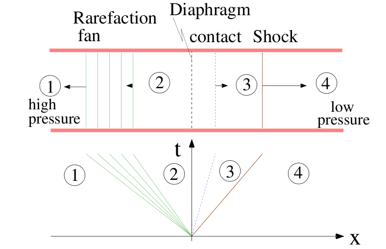
shock tube is a very long pipe in which a strong shock wave is generated. In the initial configuration, the tube is divided by a diaphragm into two compartments: the driver section containing the gas with the higher pressure $P_{1}$ and the driven section with the gas at the lower pressure $P_{4}$ .Here, we omitting the parts about reflected shock and expansion waves as well as some theory considered too general. The right-running normal shock is treated on page 21 and the solution to the complete problem is given on page 21.

We start from the continuity, momentum and energy equations for a stationary normal shock wave[3]:

\rho_{4}u_{4}=\rho_{3}u_{3}

(9.1)

P_{4}+\rho_{4}u_{4}^{2}=P_{3}+\rho_{3}u_{3}^{2}

(9.2)

h_{4}+\frac{u_{4}^{2}}{2}=h_{3}+\frac{u_{3}^{2}}{2}

(9.3)

where the index 4 refers to gas upstream of the wave, index 3 to gas downstream of the wave.The important point is that $u_{4}$ and $u_{3}$ are interpreted as velocities relative to the wave; because it is stationary, they are in this case also relative to the laboratory. For the moving wave the velocities relative to the wave are $W$ (for the gas ahead) and $W-u_{p}$ (for the gas behind) also making the total velocity equal to $W-u_{4}$ because In figure, with the shock wave propagating to the right . After replacing $u_{4}$ and $u_{3}$ , equation 9.1 to 9.3 become

\rho_{4}\left(W-u_{4}\right)=\rho_{3}\left(W-u_{p}\right)

(9.4)

P_{4}+\rho_{4}\left(W-u_{4}\right)^{2}=P_{3}+\rho_{3}\left(W-u_{p}\right)^{2}

(9.5)

h_{4}+\frac{\left(W-u_{4}\right)^{2}}{2}=h_{3}+\frac{\left(W-u_{p}\right)^{2}}{2}

(9.6)

Equations 9.4 to 9.6 are the normal-shock equations for a shock moving with velocity W into a stagnant gas. They can be rearranged and substituted, using h = e+p/ $\rho$ , to obtain

e_{3}-e_{4}=\frac{P_{4}+P_{3}}{2}\left(V_{4}-V_{3}\right)

(9.7)

The states after the shock are connected by the Rankine Hugoniot shock jump conditions[9] (Landau page no. 334) is valid, because we assume the case of polytropic gas, $e=C_{P}T$ , $T=\frac{PV}{R}$ and $V=\frac{1}{\rho}$ ; equation 9.7 becomes

\boxed{\frac{V_{3}}{V_{4}}=\frac{P_{3}}{P_{4}}\Bigg{(}\frac{\frac{\gamma+1}{\gamma-1}+\frac{P_{3}}{P_{4}}}{1+\frac{\gamma+1}{\gamma-1}}\Bigg{)}}

(9.8)

\boxed{\Rightarrow\frac{\rho_{3}}{\rho_{4}}=\frac{\frac{\gamma+1}{\gamma-1}+\frac{P_{3}}{P_{4}}}{1+\frac{\gamma+1}{\gamma-1}}}

(9.9)

Equations 9.8 and 9.9 give the temperature and density ratios across the shock wave as functions of the pressure ratio. We define the moving shock Mach number as

Ma_{S}=\frac{W-u_{4}}{a_{4}}

By taking the polytropic gas relations and Eqn. 9.4 to 9.6 into account, we can derive

\frac{P_{3}}{P_{4}}=1+\frac{2\gamma}{\gamma+1}\left(Ma_{S}^{2}-1\right)

\Rightarrow Ma_{S}=\sqrt{\frac{\gamma+1}{2\gamma}\left(\frac{P_{3}}{P_{4}}-1\right)+1}

(9.10)

Since $Ma_{S}=(W-u_{4})/a_{4}$ , Eqn. 9.10 leads to

W-u_{4}=a_{4}\sqrt{\frac{\gamma+1}{2\gamma}\left(\frac{P_{3}}{P_{4}}-1\right)+1}

(9.11)

Equation 9.11 relates the velocity of the moving shock wave to the pressure ratio across the wave and the local speed of sound of the gas ahead of the shock wave.

The last quantity we are interested in is the velocity up of the mass motion induced by the shock wave. Equation 9.4 can be rewritten

\boxed{u_{p}=W+\left(W-u_{4}\right)\left(-\frac{\rho_{4}}{\rho_{3}}\right)}

(9.12)

After substitution of Eqn. 9.9 and 9.11 into Eqn. 9.12, we obtain

\boxed{u_{p}=u_{4}+\frac{a_{4}}{\gamma}\left(\frac{P_{3}}{P_{4}}\right)\left(\frac{\frac{2\gamma}{\gamma+1}}{\frac{P_{3}}{P_{4}}+\frac{\gamma-1}{\gamma+1}}\right)^{1/2}}

(9.13)

With what we have derived so far, we can obtain for a given pressure ratio $P_{3}/P_{4}$ and speed of sound $a_{4}$ the corresponding values of $\rho_{3}/\rho_{4}$ , $T_{3}/T_{4}$ , W and up from Eqn 9.8, 9.9, 9.11 and 9.13. The next section deals with the counterpart of the moving shock wave, namely the expansion wave.

9.1 The incident expansion wave

In the last section discussions about the relations between the regions 3 and 4 of Fig. 6. In this section we examine the regions 1 and 2. The formulas relate to a left-running expansions wave; they would be similar for a right-running one except some changes of the signs in the equations. We use the fact that the gas in region 1 feels as if a piston was pulled to the right with velocity $u_{4}$ . In fact, $u_{4}$ is the mass-motion velocity of the gas behind the expansion wave[3] because this portion is high pressure region realtive to region 4.

Inside the wave, a mass motion with velocity u is induced, directed toward right. Temperature T and subsequently the local speed of sound a are reduced; because of this the head of the wave propagates faster into region 1 than other parts of the wave, so the wave is spreading out while running down the tube.

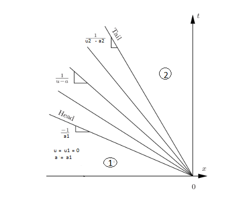
The tail of the wave moves at velocity $dx/dt=u_{2}-a_{2}$ . Note that if $u_{2}>a_{2}$ , i. e., $u_{2}$ is supersonic, the tail of the wave propagates to the right although the wave is left-running. It can be shown that the characteristics of the expansion wave are straight lines and thus the values of u, a (and consequently also p, $\rho$ , T etc.) are constant along them. Such a wave is called a simple wave; a non simple waves where the characteristics are curved comes up for example when the expansion wave is reflected.

To obtain a closed analytical form for the expansion wave, we use Riemann invariant form [9] (page no. 394)

u+\frac{2a}{\gamma-1}=\text{constant through the wave}

(9.14)

Applying this equation in region 1, we get

u_{1}+\frac{2a_{1}}{\gamma-1}=\text{constant}

(9.15)

Combining these equations we get

\boxed{\frac{a}{a_{1}}=1-\frac{\gamma-1}{2}\left(\frac{u}{a_{1}}-\frac{u_{1}}{a_{1}}\right)}

(9.16)

Which relates u and a within the expansion wave. Because $a=\sqrt{\gamma RT}$ Eqn 9.16 also gives

\frac{T}{T_{1}}=\left(1-\frac{\gamma-1}{2}\left(\frac{u}{a_{1}}-\frac{u_{1}}{a_{1}}\right)\right)^{2}

(9.17)

For isentropic process $\triangle s=0$

P=(\text{constant})\rho^{\gamma},\hskip 8.53581ptT=(\text{constant})\rho^{\gamma-1}\hskip 8.53581pt,a=(\text{constant})\rho^{(\gamma-1)/2}

Then from Eqn. 9.17, we get

\boxed{\frac{P}{P_{1}}=\left(1-\frac{\gamma-1}{2}\left(\frac{u}{a_{1}}-\frac{u_{1}}{a_{1}}\right)\right)^{2\gamma/(\gamma-1)}}

(9.18)

and

\boxed{\frac{\rho}{\rho_{1}}=\left(1-\frac{\gamma-1}{2}\left(\frac{u}{a_{1}}-\frac{u_{1}}{a_{1}}\right)\right)^{2/(\gamma-1)}}

(9.19)

These equations give all properties within the simple expansion wave as a function of the local gas velocity u. To get them as function of x and t, we use straight line characteristics as

\frac{dx}{dt}=\left(u-a\right)t

\Rightarrow x=\left(u-a\right)t+u_{1}

Using this relation in Eqn. 9.16

x=\left(u-u_{1}-a_{1}+\frac{\gamma-1}{2}u\right)t

\boxed{\Rightarrow u=u_{1}+\frac{2}{\gamma-1}\left(a_{1}+\frac{x}{t}\right)}

(9.20)

The properties can be determined within the expansion wave, $u_{1}-a_{1}\leqslant x/t\leqslant u_{2}-a_{2}$

9.2 Final Expression of Shock Tube

Finally, we combine the last two section for a closed analytical solution. End of the day we recall that $u_{2}=u_{3}=u_{p}$ and $P_{2}=P_{3}$ across the contact surface; last expression of $u_{p}$ was

u_{p}=u_{3}=u_{4}+\frac{a_{4}}{\gamma}\left(\frac{P_{3}}{P_{4}}\right)\left(\frac{\frac{2\gamma}{\gamma+1}}{\frac{P_{3}}{P_{4}}+\frac{\gamma-1}{\gamma+1}}\right)^{1/2}

Applying Eqn. 9.18 to the tail of the expansion wave,

\frac{P_{2}}{P_{1}}=\left(1-\frac{\gamma-1}{2}\Big{(}\frac{u_{2}}{a_{1}}-\frac{u_{1}}{a_{1}}\Big{)}\right)^{2\gamma/(\gamma-1)}

(9.21)

\Rightarrow u_{2}=u_{1}+\frac{2a_{1}}{\gamma-1}\left(1-\Big{(}\frac{P_{2}}{P_{1}}\Big{)}^{(\gamma-1)/2\gamma}\right)

Putting $P_{2}=P_{3}$

u_{2}=u_{1}+\frac{2a_{1}}{\gamma-1}\left(1-\Big{(}\frac{P_{3}}{P_{1}}\Big{)}^{(\gamma-1)/2\gamma}\right)

Since $u_{2}=u_{3}$ , so we apply in last Eqn. and equation 9.13, we get

u_{4}+\frac{a_{4}}{\gamma}\bigg{(}\frac{P_{3}}{P_{4}}\bigg{)}\Bigg{(}\frac{\frac{2\gamma}{\gamma+1}}{\frac{P_{3}}{P_{4}}+\frac{\gamma-1}{\gamma+1}}\Bigg{)}^{1/2}=u_{1}+\frac{2a_{1}}{\gamma-1}\left(1-\Big{(}\frac{P_{3}}{P_{1}}\Big{)}^{(\gamma-1)/2\gamma}\right)

\boxed{\frac{P_{4}}{P_{1}}=\frac{P_{4}}{P_{3}}\left(1+\frac{\big{(}u_{1}-u_{4}\big{)}\big{(}\gamma-1\big{)}}{2a_{1}}-\frac{\Big{(}\gamma-1\Big{)}\Big{(}\frac{a_{4}}{a_{1}}\Big{)}\Big{(}\frac{P_{3}}{P_{4}}-1\Big{)}}{\sqrt{2\gamma\Bigg{(}\Big{(}\gamma-1\Big{)}+\Big{(}\gamma+1\Big{)}\frac{P_{3}}{P_{4}}\Bigg{)}}}\right)^{2\gamma/(\gamma-1)}}

(9.22)

Equation (9.22) gives the incident shock strength $P_{3}/P_{4}$ as an implicit function of the diaphragm pressure ratio $P_{1}/P_{4}$ . We can now unfold a recipe for the solution of the shock tube problem, which consists of all the boxed equations:

$\ast$

Calculate $P_{3}/P_{4}$ from Eqn. 9.22 to get the strength of the shock wave.
$\ast$

Calculate all other shock properties from Eqn. 9.8, 9.9, 9.11 and 9.13.
$\ast$

Calculate $P_{2}/P_{1}=(P_{2}/P_{4})/(P_{1}/P_{4})=(P_{3}/P_{4})/(P_{1}/P_{4})$ to get the strength of the expansion wave.
$\ast$

All other properties behind the expansion wave can be found using

$\frac{P_{2}}{P_{1}}=\left(\frac{\rho_{2}}{\rho_{1}}\right)^{\gamma}$
$\ast$

The properties inside the expansion wave can be found from Eqs. 9.16 to 9.19 and 9.20.

9.3 Implementation in Python

Source code of these mathematics is given in section 13.3, where xgrid is a vector containing the x-positions where the solution is evaluated rho , u ,c(=a),P,machE and $entropy\_E$ are vectors of the size of x_grid containing the density, local velocity,sound velocity,pressure, Mach number and entropy at the corresponding positions.

$t\_end$ specifies at what time the solution is to be evaluated;rhoL( $=\rho_{1}$ ), rhoR $(=\rho_{4})$ , PrL $(P_{1})$ , PrR $(=P_{4})$ , uL = $u_{1}$ uR = $u_{4}$ initial settings for density, pressure and local velocity in the two compartments.

After parsing the input and optionally setting default values, some constants are specified: the heat capacity gamma = 1.4 and position of diaphragm at 0.5 . Next local speed and the densities for region 1 and 4 are computed from the quantities known so far. To get P3, rho3, rho2, u2 and c2 we solve Eqn 9.22 for $P_{3}/P_{4}$ that means we have to find a $P_{3}/P_{4}$ satisfying

\frac{P_{4}}{P_{3}}\left(1+\frac{\big{(}u_{1}-u_{4}\big{)}\big{(}\gamma-1\big{)}}{2a_{1}}-\frac{\Big{(}\gamma-1\Big{)}\Big{(}\frac{a_{4}}{a_{1}}\Big{)}\Big{(}\frac{P_{3}}{P_{4}}-1\Big{)}}{\sqrt{2\gamma\Bigg{(}\Big{(}\gamma-1\Big{)}+\Big{(}\gamma+1\Big{)}\frac{P_{3}}{P_{4}}\Bigg{)}}}\right)^{2\gamma/(\gamma-1)}-\frac{P_{4}}{P_{1}}=0

(9.23)

This equation is solved by python function fsolve which can gives the iterative solution about a point of iterative solution by using Newton’s method, bisection method etc.

Now, the mesh $x\_grid$ is initialized, usually to a size of 1 x 300, but the number of points could also be changed to some other value if desired. Before iterating through all the solution vectors, the boundaries of the regions are determined using the knowledge about the velocities of head and tail of the expansion wave.

$\ast$

Starting expansion fan i.e Boundary between leftmost driver gas and expansion wave.

$pos1=0.5+(u_{1}-a_{1})*t\_end$

$\Rightarrow pos1=0.5+(uL-aL)*t\_end$
$\ast$

End of expansion fan i.e. Boundary between expansion wave and lower pressure driver gas.

$pos2=0.5+(u_{3}-a_{3})*t\_end$

$\Rightarrow pos2=0.5+(u2+uR-c2)*t\_end\hskip 8.53581pt\text{, because u2 = u3}$
$\ast$

Position of contact discontinuity i.e. Boundary between driver gas and driven gas.

$conpos=0.5+u\_p*t\_end$

$\Rightarrow conpos=0.5+(u2+uR)*t\_end$

\ast

Shock Position i.e Location of the shock wave.

spos=0.5+t\_end*W

\Rightarrow spos=0.5+t\_end*\left(a_{4}\sqrt{\frac{\gamma+1}{2\gamma}\left(\frac{P_{3}}{P_{4}}-1\right)+1}+u_{4}\right)

\Rightarrow spos=0.5+t\_end*\left(a_{4}\sqrt{\frac{\gamma-1}{2\gamma}+\frac{\gamma+1}{2\gamma}\frac{P_{3}}{P_{4}}}+u_{4}\right)

\Rightarrow spos=0.5+t\_end*\left(cR\sqrt{\frac{\gamma-1}{2\gamma}+\frac{\gamma+1}{2\gamma}\frac{P3}{P4}}+uR\right)

10 Sod Shock Tube

The Sod shock tube problem, named after Gary A. Sod, is a common test for the accuracy of computational fluid codes, like Riemann solvers and was heavily investigated by Sod in 1978. The test consists of a one dimensional Riemann problem with the following parameters, for left and right states of an ideal gas.

\begin{pmatrix}\rho_{L}\\ u_{L}\\ P_{L}\end{pmatrix}=\begin{pmatrix}1.0\\ 0.0\\ 1.0\end{pmatrix}\begin{pmatrix}\rho_{R}\\ v_{R}\\ P_{R}\end{pmatrix}=\begin{pmatrix}0.125\\ 0.0\\ 0.1\end{pmatrix}

(10.1)

The time evolution of this problem can be described by solving the Euler equations. Which leads to three characteristics, describing the propagation speed of the various regions of the system. Namely the rarefaction wave, the contact discontinuity and the shock discontinuity. If this is solved numerically, one can test against the analytical solution, and get information how well a code captures and resolves shocks and contact discontinuities and reproduce the correct density profile of the rarefaction wave.

11 Result:

11.1 Shock tube Data Plot after Breaking the Diaphragm

In this case

$t\_end$ =0.17 Sec N=300 $\mu$ =0.35
Quantity	left side	right side
Density	1.0	0.125
Pressure	1.0	0.1
Velocity	0.0	0.0

Table 1: Shock tube data at t = 0

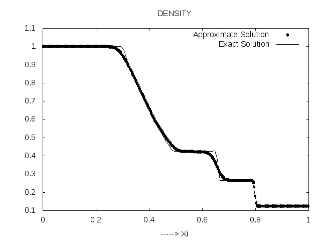
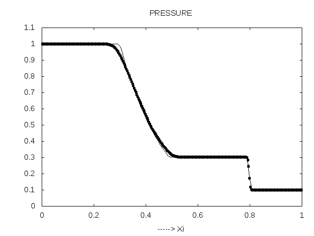
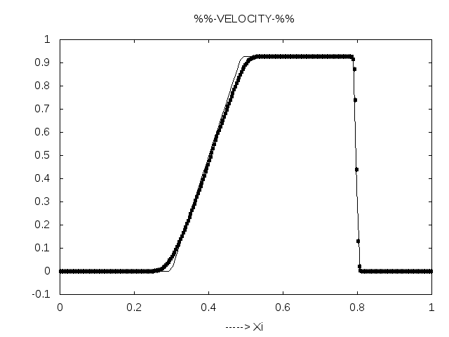
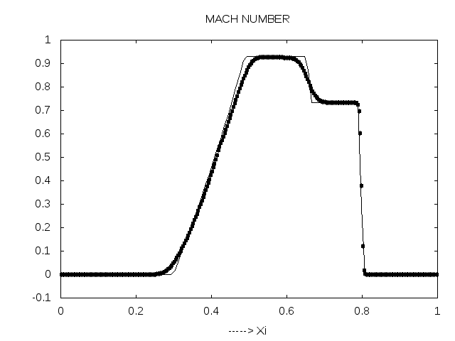
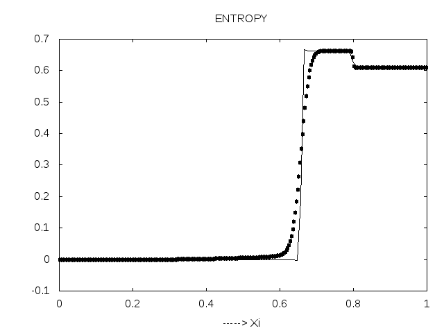
Comparison to measurements yields respectable results, actually this result is only for stationary shock tube.but our program simulation for both cases. Three Python scripts on the accompanying movies, which visualize the density,pressure,velocity, Mach number and entropy in shock tube after breaking the diaphragm.See Appendix LABEL:subsec:_Contents_in_CD for details on the CD.

Script file	Video file	Quantity
exact.py	exact.avi	Exact value by Shock tube formula
approximate.py	approximate.avi	Approximate solution by Roe Solver
approximate_exact.py	approximate_exact.avi	Both solution

Table 2: Scripts for video files visualizing the analytical and approximate solution

12 Conclusions

We described a strategy for obtaining numerical solutions to hyperbolic initial-value problems by Roe Scheme Method[1]. In the project we have the details of one element in that strategy. Our investigations into the Euler equations have revealed some very tidy structures. Also the existence of a fast exact Riemann solver is found more generally useful. Our programming experience is that the present direct method is about a time-consuming as one cycle of the iterative procedures. Iterations needed to obtain more exact solutions. Also we use Harten entropy fix assuming the Harten original approach: the entropy fix as means to select the physically relevant weak solution, corresponding to the vanishing viscosity solution.

13 Appendix

13.1 Implementation in Python of Roe Scheme:

we will apply the Roe Scheme to the one test case of shock tube. We discretize the flow of quantity u by finite volume method of equation 7.7 in time by explicit Euler method

\bar{u}_{i}(t_{2})=\bar{u}_{i}(t_{1})-\frac{\triangle t}{\triangle x_{i}}[F_{i+1/2}-F_{i-1/2}]

\Rightarrow\bar{u}_{i}(t_{2})=\bar{u}_{i}(t_{1})-\nu[F_{i+1/2}-F_{i-1/2}]

(13.1)

The exact solution is used to prescribe $u_{1}(t)$ and $u_{i}(t)$ . The time step $\triangle t$ and mesh size $\triangle x_{i}$ ’s are constant .

$\ast$

Grid of Physical Quantity Take x_grid, density grid, pressure grid, velocity grid all have same no of grid point(in our case 300) last three grid maintain Riemann Problem given in equation 8.2 i.e. first half grid value will rhoL, PrL, uL and last half grid value rhoR, PrR, uR.
$\ast$

Energy Momentum Calculate total energy, momentum, total enthalpy by using equation 8.8 and 8.9
$\ast$

Average Calculation Calculate density average velocity, enthalpy average by using equation 8.18 and 8.19 similarly calculate the flux averages and apply on all grid point.
$\ast$

Grid of New Average Calculation From this new grid calculate Aav by using equation 8.11 also alpha1,Eqn 8.25 alpha2, 8.24 alpha3 8.26, lambda’s 8.21 now we have all the eigenvalues and corresponding eigenvector but to remove the problem of artificial viscosity apply Harten sonic entropy fix condition 8.28
$\ast$

Flux Average Calculate roe flux’s Eqn 8.27 where for 1st term is flux averages.
$\ast$

Average data for grid formation since we have the average data between two grid point so we can fill centering grid point by using 13.1 , which is our new grid.
$\ast$

Entropy End of the program calculate entropy

$entropy=log(P/\rho**\gamma)$

Since at t = 0 all left and right side data are same so when we calculate the average value gives us ’-nan’ so next time gives two ’-nan’ data so it will be dangerous. To remove this problem if $U_{i}==-nan$ then $U_{i}=U_{i-1}$ .

13.2 Python Code

⬇

#!/usr/bin/env python

"""

Roe Scheme for one-dimensional Euler equations of Perfect

Gas in Adiabatic Process....

"""

import numpy as np

from pylab import *

from decimal import *

""" -----o---Specification of Riemann problems---o--- """

PrL = 1.0; PrR = 0.1; rhoL = 1.0; rhoR = 0.125;

uL = 0; uR = 0; t_end = 0.17; mu = 0.35; # nu = dt/dx

""" -------- Input Section -------- """

gamma = 1.4 # Ratio of specific heat

N = 300.0 # Number of grid cells

"""-------END I/P ----- """

gammaA = gamma - 1 ; gammaB = 1/(gamma - 1)

dx = 1/N # Cell Size

dt = mu*dx # Time step

n = int(t_end/dt)

"""

Definition of grid numbering

x=0 x=1

grid |--o--|--o--|--o--|--o-- .... ---|--o--|

1 1 2 2 3 3 4 N-1 N I

"""

N = int(N)

x = np.linspace(0.0,1.0,N+1)

xgrid = np.linspace(dx,1.0,N) - (dx/2)

Pr = np.zeros((1,len(xgrid)))

rho = np.zeros((1,len(xgrid)))

u = np.zeros((1,len(xgrid)))

for i in range (0, N, 1):

if xgrid[i] < 0.5 : Pr[0,i] = PrL; rho[0,i] = rhoL; u[0,i] = uL

else: Pr[0,i] = PrR; rho[0,i] = rhoR; u[0,i] = uR

eI = (gammaB*Pr)/rho # specific (= per unit mass) internal energy

eT = gammaB*Pr # Thermal energy

M = u*rho # Momntum rho*u

Et = eT + 0.5*M* u # Total energy

EtL = Et[0,0] ; EtR = Et[0,N-1]

Ht = gamma*eI + 0.5*u*u # Total enthalpy

# New cell centre Variables

mach = np.zeros((1,N))

rho_n = np.zeros((1,N))

M_n = np.zeros((1,N))

Et_n = np.zeros((1,N))

A_n = np.zeros((1,N))

# Roe Fluxes

roeF1 = np.zeros((1,N))

roeF2 = np.zeros((1,N))

roeF3 = np.zeros((1,N))

# Roe Averages

Hav = np.zeros((1,N))

uav = np.zeros((1,N))

Aav = np.zeros((1,N))

dd = np.zeros((1,N))

# Flux Averages

F1av = np.zeros((1,N))

F2av = np.zeros((1,N))

F3av = np.zeros((1,N))

# State Vector Difference

delrho = np.zeros((1,N))

delM = np.zeros((1,N))

delEt = np.zeros((1,N))

# Eigenvalues

lamda1 = np.zeros((1,N))

lamda2 = np.zeros((1,N))

lamda3 = np.zeros((1,N))

#Coefficents

alpha1 = np.zeros((1,N))

alpha2 = np.zeros((1,N))

alpha3 = np.zeros((1,N))

t = 0

for i in range (0,n,1):

t = t + dt

for j in range(0,N-2,1):

dd[0,j] = np.sqrt(rho[0,j+1]/rho[0,j])

if np.isnan(dd[0,j]) == True:

dd[0,j] = dd[0,j-1]

Hav[0,j] = (Ht[0,j] + dd[0,j]*Ht[0,j+1])/(1+dd[0,j])

uav[0,j] = (u[0,j] + dd[0,j]*u[0,j+1])/(1+dd[0,j])

delrho[0,j] = rho[0,j+1] - rho[0,j]

delM[0,j] = M[0,j+1] - M[0,j]

delEt[0,j] = Et[0,j+1] - Et[0,j]

F1av[0,j] = 0.5*(M[0,j] + M[0,j+1])

F2av[0,j] = 0.5*((M[0,j]*M[0,j]/rho[0,j]) + Pr[0,j] +

(M[0,j+1]*M[0,j+1]/rho[0,j+1]) + Pr[0,j+1])

F3av[0,j] = 0.5*((M[0,j]*Ht[0,j]) + (M[0,j+1]*Ht[0,j+1]))

Aav = np.sqrt(gammaA*(Hav - 0.5*(uav*uav)))

Mav = uav/Aav

alpha1 = (0.25*Mav*(2+gammaA*Mav)*delrho -

0.5*(1+gammaA*Mav)*(delM/Aav) + 0.5*gammaA*(delEt/(Aav**2)))

alpha2 = ((1-0.5*gammaA*(Mav**2))*delrho + gammaA*(Mav/Aav)*delM -

gammaA*(delEt/(Aav**2)))

alpha3 = (-0.25*Mav*(2-gammaA*Mav)*delrho + 0.5*(1-gammaA*Mav)*(delM/Aav)

+ 0.5*gammaA*(delEt/(Aav**2)))

lamda1 = np.abs(uav - Aav); lamda2 = np.abs(uav);

lamda3 = np.abs(uav + Aav)

""" Harten’s sonic entropy fix """

Eps = 0.5

""" Eps = 0.0 No entropy fix """

for j in range (0,N-1):

if lamda1[0,j] < Eps :

lamda1[0,j] = 0.5*((Eps + lamda1[0,j]**2)/Eps)

if lamda3[0,j] < Eps:

lamda3[0,j] = 0.5*((Eps + lamda3[0,j]**2)/Eps)

roeF1 = F1av - 0.5*lamda1*alpha1 - 0.5*lamda2*alpha2 - 0.5*lamda3*alpha3

roeF2 = (F2av - 0.5*lamda1*alpha1*(uav-Aav) - 0.5*lamda2*alpha2*uav

- 0.5*lamda3*alpha3*(uav+Aav))

roeF3 = (F3av - 0.5*lamda1*alpha1*(Hav - uav*Aav) - 0.25*lamda2*

alpha2*uav*uav- 0.5*lamda3*alpha3*(Hav + uav*Aav))

rho_n[0,0] = rhoL; rho_n[0,N-1] = rhoR

M_n[0,0] = rhoL*uL; M_n[0,N-1] = rhoR*uR

Et_n[0,0] = EtL; Et_n[0,N-1] = EtR

for j in range(1, N-1):

rho_n[0,j] = rho[0,j] - mu*(roeF1[0,j] - roeF1[0,j-1])

M_n[0,j] = M[0,j] -mu*(roeF2[0,j] - roeF2[0,j-1])

Et_n[0,j] = Et[0,j] - mu*(roeF3[0,j] - roeF3[0,j-1])

u = M_n/rho_n

Pr = gammaA*(Et_n - 0.5*M_n*u)

eI = (gammaB*Pr)/rho_n

Ht = (Et_n + Pr)/rho_n

rho = rho_n

M = M_n

Et = Et_n

A_n = np.sqrt(gamma*gammaA*eI)

mach = u/A_n

for k in range(1,N):

if np.isnan(u[0,k]) == True:

u[0,k] = u[0,k-1]

if np.isnan(Pr[0,k]) == True:

Pr[0,k] = Pr[0,k-1]

if np.isnan(eI[0,k]) == True:

eI[0,k] = eI[0,k-1]

if np.isnan(Ht[0,k]) == True:

Ht[0,k] = Ht[0,k-1]

if np.isnan(rho[0,k]) == True:

rho[0,k] = rho[0,k-1]

if np.isnan(M[0,k]) == True:

M[0,k] = M[0,k-1]

if np.isnan(Et[0,k]) == True:

Et[0,k] = Et[0,k-1]

ent_ropy = np.log(Pr/(rho**gamma))

""" ---o---File Write Section---o--- """

file = open("roe_scheme.txt","w")

for i in range(0,xgrid.size):

(file.write(str("%.6f"%xgrid[0,i])+’ ’+str("%.6f"%rho_n[0,i])+’

’+str("%.6f"%Pr_n[0,i])+’ ’+str("%.6f"%u_nE[0,i])+’

’+str("%.6f"%machE[0,i])+’ ’+str("%.6f"%entropy_E[0,i])))

file.write("\n")

file.close()

13.3 Code For Sod Shock Tube Problem By Python Code:

⬇

#!/usr/bin/env python

import numpy as np

from scipy.optimize import fsolve

#--------o--Input Section--o-------

# Sod Shock Tube Problem

PrL = 1.0; PrR = 0.1; rhoL = 1.0; rhoR = 0.125;

uL = 0.0; uR = 0.0; t_end = 0.2; mu = 0.35; # mu = dt/dx

#--------o--END Input Section--o-----------------

gamma = 1.4

gammaA = gamma - 1.0

gammaB = 1/gammaA

gammaC = gamma + 1.0

PRL = PrR/PrL

cR = np.sqrt(gamma * PrR/rhoR)

cL = np.sqrt(gamma * PrL/rhoL)

CRL = cR/cL

machL = (uL - uR)/cL

def func(p34):

wortel = np.sqrt(2 * gamma * (gammaA + gammaC * p34))

yy = (gammaA * CRL * (p34 - 1)) / wortel

yy = (1 + machL * gammaA/2 - yy)**(2 * gamma/gammaA)

y = yy/p34 - PRL

return y

p34 = fsolve(func,3.0) # p34 = p3/p4

print p34

p3 = p34 * PrR

alpha = gammaC/gammaA

rho3 = rhoR * (1 + alpha * p34)/(alpha + p34)

rho2 = rhoL * (p34 * PrR/PrL)**(1/gamma)

u2 = uL-uR+(2/gammaA)*cL*(1 - (p34 * PrR/PrL)**(gammaA/(2 * gamma)))

c2 = np.sqrt(gamma * p3/rho2)

spos = (0.5 + t_end* cR *np.sqrt(gammaA/(2 * gamma) +

gammaC/(2 * gamma) * p34) + t_end * uR) # Shock position

conpos = 0.5 + u2 * t_end + t_end * uR # Position of contact discontinuity

pos1 = 0.5 + (uL - cL) * t_end # Start of expansion fan

pos2 = 0.5 + (u2 + uR - c2) * t_end # End of expansion fan

xgrid = np.linspace(0,1,100)

PrE = np.zeros((1,len(xgrid)))

uE= np.zeros((1,len(xgrid)))

rhoE = np.zeros((1,len(xgrid)))

machE = np.zeros((1,len(xgrid)))

cE = np.zeros((1,len(xgrid)))

xgrid = np.matrix(xgrid)

for i in range (0,xgrid.size):

if xgrid[0,i] <= pos1:

PrE[0,i] = PrL

rhoE[0,i] = rhoL

uE[0,i] = uL

cE[0,i]= np.sqrt(gamma*PrE[0,i]/rhoE[0,i]);

machE[0,i]= uE[0,i]/cE[0,i];

elif xgrid[0,i] <= pos2:

PrE[0,i] = (PrL*(1 + (pos1 - xgrid[0,i])

/(cL * alpha * t_end))**(2 * gamma/gammaA))

rhoE[0,i] = (rhoL*(1+(pos1 - xgrid[0,i])

/(cL * alpha * t_end))**(2/gammaA))

uE[0,i] = uL + (2/gammaC)*(xgrid[0,i] - pos1)/t_end

cE[0,i] = np.sqrt(gamma * PrE[0,i]/rhoE[0,i])

machE[0,i] = uE[0,i]/cE[0,i]

elif xgrid[0,i] <= conpos:

PrE[0,i] = p3

rhoE[0,i] = rho2

uE[0,i] = u2 + uR;

cE[0,i]= np.sqrt(gamma * PrE[0,i]/rhoE[0,i]);

machE[0,i] = uE[0,i]/cE[0,i]

elif xgrid[0,i] <= spos:

PrE[0,i] = p3

rhoE[0,i] = rho3

uE[0,i] = u2+uR

cE[0,i] = np.sqrt(gamma * PrE[0,i]/rhoE[0,i])

machE[0,i] = uE[0,i]/cE[0,i]

else:

PrE[0,i] = PrR

rhoE[0,i] = rhoR;

uE[0,i] = uR

cE[0,i] = np.sqrt(gamma*PrE[0,i]/rhoE[0,i]);

machE[0,i] = uE[0,i]/cE[0,i];

entropy_E = np.log(PrE/rhoE**gamma);

""" ---o---File Write Section---o--- """

file = open("Riemann.txt","w")

for i in range(0,xgrid.size):

(file.write("%.6f"%str(xgrid[0,i])+’ ’+str("%.6f"%rhoE[0,i])+’

’+str("%.6f"%PrE[0,i])+’ ’+str("%.6f"%uE[0,i])+’

’+str("%.6f"%machE[0,i])+’ ’+str("%.6f"%entropy_E[0,i])))

file.write("\n")

file.close()

An Introduction to Fluid Dynamics and Numerical Solution of Shock Tube Problem by Using Roe Solver

Acknowledgements

Abstract

1 Introduction

1.1 What is a Fluid?

1.2 Newton’s Law of Viscosity:

1.3 Specification of motion

1.4 Material Derivative

2 General Transport Theorem

2.1 Control System

2.2 Reynolds Transport Theorem:

3 Conservation of Mass

4 ConservatioFconsern of Momentum

5 Energy Conservation

6 Euler Equation:

7 Finite Volume Method

8 Roe Scheme Method

8.1 Parameter Vector:

8.2 Eigenvalues and Eigenvectors for Euler Equation

8.3 Approximate Riemann Solver

8.4 Harten Sonic Entropy Fix

9 One-Dimensional Shock-Tube Problem

9.1 The incident expansion wave

9.2 Final Expression of Shock Tube

9.3 Implementation in Python

10 Sod Shock Tube

11 Result:

11.1 Shock tube Data Plot after Breaking the Diaphragm

12 Conclusions

References

13 Appendix

13.1 Implementation in Python of Roe Scheme:

13.2 Python Code

13.3 Code For Sod Shock Tube Problem By Python Code:

References

- [1] P. L. ROE JOURNAL OF COMPUTATIONAL. PHYSICS. 43, 357-372 (1981). Approximate. Riemann Solvers, Parameter Vectors, and Difference Schemes.
- [2] S. K. GHOSH ‘LECTURE ON ATMOSPHERIC SCIENCE. Fluid Mechanics‘
- [3] Anderson, Dale A., Tannehill, John C., & Pletcher, Richard H. 1984. Computational Fluid Mechanics and Heat Transfer. New York: McGraw-Hill.
- [4] T.J. PEDLEY, ’Introduction to Fluid Dynamics’, SCI. MAR., 61 (Supl. 1): 7-24
- [5] R. Eymard, T Gallouët and R. Herbin, ’FINITE VOLUME METHOD’, update of the article published in Handbook of Numerical Analysis, 2000
- [6] Elizabeth H. Hearn,’The Reynolds Transport Theorem’
- [7] P. Wesseling, Principles of Computational Fluid Dynamics
- [8] M. Pelanti, L. Quartapelle and L. Vigevano ’A review of entropy fixes as applied to Roe’s linerization’
- [9] L. D. LANDAU & E. M. LIFSHITZ ‘FLUID MECHANICS’ Second Edition