An insightful approach to bearings-only tracking in log-polar coordinates

Athena Helena Xiourouppa 0000-0003-0033-744X Dmitry Mikhin Melissa Humphries 0009-0002-6228-2958 0000-0002-0473-7611 and John Maclean 0000-0002-5533-0838

Abstract

The choice of coordinate system in a bearings-only (BO) tracking problem influences the methods used to observe and predict the state of a moving target. Modified Polar Coordinates (MPC) and Log-Polar Coordinates (LPC) have some advantages over Cartesian coordinates. In this paper, we derive closed-form expressions for the target state prior distribution after ownship manoeuvre: the mean, covariance, and higher-order moments in LPC. We explore the use of these closed-form expressions in simulation by modifying an existing BO tracker that uses the UKF. Rather than propagating sigma points, we directly substitute current values of the mean and covariance into the time update equations at the ownship turn. This modified UKF, the CFE-UKF, performs similarly to the pure UKF, verifying the closed-form expressions. The closed-form third and fourth central moments indicate non-Gaussianity of the target state when the ownship turns. By monitoring these metrics and appropriately initialising relative range error, we can achieve a desired output mean estimated range error (MRE). The availability of these higher-order moments facilitates other extensions of the tracker not possible with a standard UKF.

Index Terms:

Statistical analysis, bearings-only tracking, target tracking, Modified Polar Coordinates, Log-Polar Coordinates, Unscented Kalman Filter

I Introduction

Consider a sensing platform (ownship) tracking a vessel of interest (target) using a passive acoustic sensor.¹¹1For simplicity, we ignore the potential differences between the ownship coordinates / orientation and the sensor coordinates / orientation. Assume energy propagates in simple, horizontal straight lines, so that there is only one energy path (ray) from target to sensor. The sensor obtains the target bearing by measuring the direction of target noise arrival. We aim to recover the target’s full state, i.e., position and speed, from a sequence of this data.

Modified Polar Coordinates (MPC) have been established as a stable approach for bearings-only (BO) target tracking. State update equations in MPC are non-linear; to implement estimation for non-linear systems, existing literature suggests the use of the Extended Kalman Filter (EKF) [1, 2] or Unscented Kalman Filter (UKF) [3].

Log-Polar Coordinates (LPC) are another viable candidate [4, 5], especially for theoretical analysis; using LPC, one can obtain the posterior Cramér-Rao bound (PCRB) for the target state distribution [4]. This paper further explores the theoretical properties of the state distribution in LPC.

We do so in the context of a simple explicit ownship manoeuvre, described in Section II; broader scenarios can be approximated as combinations of simple manoeuvres.

The main contribution of this paper is proving that the target state distribution after an ownship manoeuvre can be described in LPC with closed-form expressions, derived in Section III. Closed-form expressions allow us to better understand the relationships between target state variables. We demonstrate the advantage of this for tracking simulation in Section IV by implementing a Kalman Filter that incorporates the closed-form expressions, CFE-UKF, and comparing its capabilities to a pure UKF. Conclusions are presented in Section V.

II Passive Bearings-Only Tracking

II-A Straight Line Movement

The target’s state in MPC [2] is described as a vector of

•

absolute bearing $\beta$ that is the angle from the receiver to the target measured from True North,
•

bearing rate $\dot{\beta}$ ,
•

scaled range rate $\dot{\rho}=\dot{r}/r$ , where $r$ is range, and
•

inverse range $s=1/r$ .

Here and below, the upper dot denotes the derivative with respect to time.

We define the target state at time $t$ as $\bm{x}=[\beta,\dot{\beta},\dot{\rho},s]$ . If we assume that the ownship and target do not manoeuvre, the vessel trajectory in MPC is:

	$\displaystyle\beta^{+}$	$\displaystyle=\beta+\arctan{\frac{t_{\beta}}{1+t_{\rho}}},$	$\displaystyle s^{+}$	$\displaystyle=\frac{s}{\sqrt{{(1+t_{\rho})}^{2}+{t_{\beta}}^{2}}},$		(1)
	$\displaystyle\dot{\beta}^{+}$	$\displaystyle=\frac{\dot{\beta}}{{(1+t_{\rho})}^{2}+{t_{\beta}}^{2}},$	$\displaystyle\dot{\rho}^{+}$	$\displaystyle=\frac{\dot{\rho}+\Delta t(\dot{\rho}^{2}+\dot{\beta}^{2})}{{(1+t_{\rho})}^{2}+{t_{\beta}}^{2}}.$		(1)

Here $t^{+}$ is some later time, $\Delta t=t^{+}-t$ , $t_{\beta}=\dot{\beta}\Delta t$ and $t_{\rho}=\dot{\rho}\Delta t$ . The update equations in Eq. 1 are non-linear. To use these equations for target state updates in a sequential estimator, we must apply the EKF, UKF, or other advanced methods of non-linear estimation (e.g., [6]). By taking $\Delta t$ as the update interval of the EKF or UKF, Eq. 1 would define the state transition function for the filter.

The bearing transition equation $\beta^{+}$ in Eq. 1 does not contain the initial value of inverse range $s$ . Hence, we cannot determine the range from BO measurements when the ownship and target move straight.

II-B Equations of Motion for Manoeuvring Platforms

Assume that at the initial time $t$ the ownship position and speed in a fixed Cartesian coordinate system are $x_{\text{O}}$ , $y_{\text{O}}$ , $v_{x\text{O}}$ , and $v_{y\text{O}}$ , and the corresponding position and speed at a later time $t^{+}$ are $x^{+}_{\text{O}}$ , $y^{+}_{\text{O}}$ , $v^{+}_{x\text{O}}$ , and $v^{+}_{y\text{O}}$ . Define the ownship displacement vector and speed change vector as

	$\displaystyle\bm{w}_{\text{O}}$	$\displaystyle=\left[x^{+}_{\text{O}}-x_{\text{O}}-v_{x\text{O}}\Delta t,y^{+}_{\text{O}}-y_{\text{O}}-v_{y\text{O}}\Delta t\right],$		(2)
	$\displaystyle\dot{\bm{w}}_{\text{O}}$	$\displaystyle=\left[v^{+}_{x\text{O}}-v_{x\text{O}},v^{+}_{y\text{O}}-v_{y\text{O}}\right].$		(2)

Similarly, define $\bm{w}_{\text{T}}$ and $\dot{\bm{w}}_{\text{T}}$ for the target displacement. The overall acceleration-related displacement and speed change are

	$\displaystyle\bm{a}$	$\displaystyle=\bm{w}_{\text{T}}-\bm{w}_{\text{O}},$		(3)
	$\displaystyle\dot{\bm{a}}$	$\displaystyle=\dot{\bm{w}}_{\text{T}}-\dot{\bm{w}}_{\text{O}}.$		(3)

Using these definitions, target movement in MPC in the presence of target and ownship manoeuvres follows the equations

	$\displaystyle\beta^{+}$	$\displaystyle=\beta+\arctan{\frac{D_{\beta}}{D_{\rho}}},$	$\displaystyle s^{+}$	$\displaystyle=\frac{s}{{\left(D^{2}_{\beta}+D^{2}_{\rho}\right)}^{1/2}},$		(4)
	$\displaystyle\dot{\beta}^{+}$	$\displaystyle=\frac{\dot{D}_{\beta}D_{\rho}-\dot{D}_{\rho}D_{\beta}}{D^{2}_{\beta}+D^{2}_{\rho}},$	$\displaystyle\dot{\rho}^{+}$	$\displaystyle=\frac{\dot{D}_{\rho}D_{\rho}+\dot{D}_{\beta}D_{\beta}}{D^{2}_{\beta}+D^{2}_{\rho}},$		(4)

where

	$\displaystyle D_{\beta}$	$\displaystyle=t_{\beta}+s(\bm{a}\cdot\bm{n}),$	$\displaystyle\dot{D}_{\beta}$	$\displaystyle=\dot{\beta}+s(\dot{\bm{a}}\cdot\bm{n}),$		(5)
	$\displaystyle D_{\rho}$	$\displaystyle=1+t_{\rho}+s(\bm{a}\cdot\bm{q}),$	$\displaystyle\dot{D}_{\rho}$	$\displaystyle=\dot{\rho}+s(\dot{\bm{a}}\cdot\bm{q}),$		(5)

and the unit vectors $\bm{q}$ and $\bm{n}$ point from the ownship to the target and orthogonally at time $t$ :

	$\displaystyle\bm{q}$	$\displaystyle=\left[\sin{\beta},\cos{\beta}\right],$		(6)
	$\displaystyle\bm{n}$	$\displaystyle=\left[\cos{\beta},-\sin{\beta}\right].$		(6)

The bearing update equation 4 depends on the initial target range $s$ . If we know the ownship manoeuvres, we can estimate $s$ , assuming that the target moves straight. We often generalise this conclusion as “the ownship must outmanoeuvre the target to determine its range” [2]. For the non-manoeuvring target $\bm{w}_{\text{T}}=\dot{\bm{w}}_{\text{T}}=0$ , so the subscript “O” can be omitted in Eqs. 2 and 3 without causing ambiguity. From the Kalman Filter viewpoint, the acceleration-related terms $(\bm{a}\cdot\bm{n})$ , $(\dot{\bm{a}}\cdot\bm{n})$ , $(\bm{a}\cdot\bm{q})$ , and $(\dot{\bm{a}}\cdot\bm{q})$ now represent control inputs to the system.

II-C Modified Polar Coordinates Versus Log-Polar Coordinates

BO trackers commonly use bearing, bearing rate, and scaled range rate as state variables because these values are directly observable on a straight leg of the ownship [2]. The choice of the fourth state component is not fixed. One conventional choice is MPC, in which we use inverse range $s$ as the fourth coordinate, as in Sections II-A and II-B. An alternative is to select the logarithm of range $\rho=\ln r$ as the fourth state component; this gives LPC with the state vector $\bm{x}=[\beta,\dot{\beta},\dot{\rho},\rho]$ .

The choice of LPC has several theoretical advantages over MPC. Firstly, it allows the derivation of closed-form expressions for the posterior Cramér-Rao bound (PCRB) in a BO tracking problem [4]. Compared to MPC, the LPC state vector appears more intuitive because it contains two values (bearing and log-range) and their time derivatives, while MPC mixes $s$ and $\dot{\rho}$ . Also, a Gaussian distribution of the fourth state vector component $\rho$ never results in zero or negative range values, which theoretically is always possible in MPC at the tails of the distribution. A corollary is that sigma points of the UKF algorithm [7] would never end up at infeasible negative ranges.

The transition from MPC to LPC is simple: we describe the target motion in LPC by the system of differential equations

\frac{d}{dt}\begin{bmatrix}\beta\\ \dot{\beta}\\ \dot{\rho}\\ \rho\end{bmatrix}=\begin{bmatrix}\dot{\beta}\\ -2\dot{\beta}\dot{\rho}\\ \dot{\beta}^{2}-\dot{\rho}^{2}\\ \dot{\rho}\end{bmatrix},

(7)

obtained from Eqs. (11) and (18) of [2] by substituting $s=e^{-\rho}$ . The same substitution into Eqs. 1, 4 and 5 provides the solutions of Eq. 7 for straight and manoeuvring vessels, respectively. For use in the UKF, one should also adapt the range-related elements of the process noise matrix $Q$ .

In accordance with Kalman Filter theory assumptions, we model the target state vector in LPC, $\bm{x}=[\beta,\dot{\beta},\dot{\rho},\rho]$ as a Gaussian random variable:

\bm{x}\sim\mathcal{N}(\bm{x};\bm{\mu},\Sigma).

(8)

With LPC in mind, we return to the equations of motion and make a key simplification.

II-D Instant Manoeuvres

Assume that the ownship makes an elementary manoeuvre: an instant turn. The state space variables after the manoeuvre, $[\beta^{+},\dot{\beta}^{+},\dot{\rho}^{+},\rho^{+}]$ , are related to the corresponding values before the turn, $[\beta,\dot{\beta},\dot{\rho},\rho]$ by Eqs. 4 and 5 with $\Delta t=0$ . The target coordinates and speed do not change, and neither do the ownship coordinates, as the turn is instant. Therefore, the only non-zero acceleration-related term is $\dot{\bm{a}}=-\dot{\bm{w}}=-\left[\Delta v_{x},\Delta v_{y}\right]$ , and Eq. 4 simplifies to

	$\displaystyle\beta^{+}$	$\displaystyle=\beta,$	$\displaystyle\rho^{+}$	$\displaystyle=\rho,$		(9)
	$\displaystyle\dot{\beta}^{+}$	$\displaystyle=\dot{\beta}-\frac{(\dot{\bm{w}}\cdot\bm{n})}{r},$	$\displaystyle\dot{\rho}^{+}$	$\displaystyle=\dot{\rho}-\frac{(\dot{\bm{w}}\cdot\bm{q})}{r}.$		(9)

The properties of instant manoeuvres can be used to model non-instant, gradual manoeuvres by discretisation. Any ownship trajectory can be approximated as a series of instant manoeuvres interwoven with straight leg motion. The total cumulative duration of the straight legs should equal the duration of the original complete manoeuvre. Using sufficiently short legs, we can achieve the desired accuracy of approximation.

With all the preliminaries in place, we now begin to explore the state space distribution from a statistical perspective.

III Closed-Form Expressions for the Post-Manoeuvre Distribution

III-A The Post-Manoeuvre Distribution

Gaussian approximations of the distribution of state space variables are ubiquitous in filtering, for example, when using UKF [7] or ensemble methods [8]. Assume the pre-manoeuvre distribution of the state space variables is Gaussian. What about the post-manoeuvre distribution?

Proposition 1 (Post-manoeuvre distribution).

Let $f_{x}$ refer to the pre-manoeuvre probability distribution function for the target in coordinates $\bm{x}$ (either MPC or LPC). Then, the post-manoeuvre distribution is given by

f_{x^{+}}(\bm{x}^{+})=f_{x}(\bm{h}^{-1}(\bm{x}^{+})),

where

\bm{h}^{-1}(\bm{x}^{+})=\begin{bmatrix}\beta^{+}\\ \dot{\beta}^{+}+f_{1}(\beta^{+},\rho^{+})\\ \dot{\rho}^{+}+f_{2}(\beta^{+},\rho^{+})\\ \rho^{+}\end{bmatrix},

(10)

and


$\displaystyle f_{1}(\beta,\rho)$	$\displaystyle=e^{-\rho}(\Delta v_{x}\cos\beta-\Delta v_{y}\sin\beta),$	(11a)
$\displaystyle f_{2}(\beta,\rho)$	$\displaystyle=e^{-\rho}(\Delta v_{x}\sin\beta+\Delta v_{y}\cos\beta).$	(11b)

If working in MPC, then the fourth coordinate of $\bm{x}^{+}$ is $s^{+}$ and factors $e^{-\rho}$ in $f_{1}$ and $f_{2}$ are rewritten as $s$ .

Proof.

Define the coordinate transformation by Eq. 9 from the pre-manoeuvre distribution in $\bm{x}$ to the post-manoeuvre distribution in $\bm{x}^{+}$ , as the mapping $\bm{h}(\bm{x})$ :

\bm{h}(\bm{x})=\begin{bmatrix}\beta\\ \dot{\beta}-f_{1}(\beta,\rho)\\ \dot{\rho}-f_{2}(\beta,\rho)\\ \rho\end{bmatrix}.

(12)

By observation, $\bm{h}^{-1}$ defined in the proposition is the inverse of $\bm{h}$ . The multivariate change of variable theorem then expresses the post-manoeuvre distribution:

f_{x^{+}}(\bm{x}^{+})=f_{x}(\bm{h}^{-1}(\bm{x}^{+}))\lvert\det\mathcal{J}(\bm{x}^{+})\rvert,

(13)

where $\mathcal{J}$ is the Jacobian matrix

\mathcal{J}(\bm{x}^{+})=\begin{bmatrix}1&0&0&0\\ -f_{2}(\beta,\rho)&1&0&-f_{1}(\beta,\rho)\\ f_{1}(\beta,\rho)&0&1&-f_{2}(\beta,\rho)\\ 0&0&0&1\\ \end{bmatrix}.

It is easy to check that $\mathcal{J}$ has determinant $1$ , so Eq. 13 reduces to the appropriate form. ∎

As the transformation by Eq. 12 does not alter the bearing $\beta^{+}$ or the range coordinate ( $\rho^{+}$ or $s^{+}$ ), we anticipate that the marginal post-manoeuvre distribution of these two variables is unchanged from the pre-manoeuvre distribution. Information about the target range comes from the entanglement of $\rho^{+}$ or $s^{+}$ with $\dot{\beta}^{+}$ and $\dot{\rho}^{+}$ . We now lay out some special cases in which the post-manoeuvre distribution can be found exactly.

Proposition 2.

Assume that the pre-manoeuvre distribution (in either LPC or MPC) is well approximated by the Gaussian distribution $\bm{x}\sim\mathcal{N}(\bm{\mu},\Sigma)$ , so Proposition 1 provides

f_{x^{+}}(\bm{x}^{+})\propto\text{exp}\left\{-\frac{1}{2}\left[\bm{y}^{\text{T}}\Sigma^{-1}\bm{y}\right]\right\},

(14)

where $\bm{y}=h^{-1}(\bm{x}^{+})-\bm{\mu}$ .

(1)

If the coordinate system is MPC, $x_{4}=s$ , then

(i)

the post-manoeuvre distribution is non-Gaussian, but

(ii)

the post-manoeuvre distribution is Gaussian if conditioned on the bearing rate $\beta$ . In this case, the post-manoeuvre distribution in MPC is

\begin{pmatrix}\dot{\beta}\\ \dot{\rho}\\ s\end{pmatrix}\sim\mathcal{N}\left(\begin{pmatrix}\mu_{\dot{\beta}}-c_{1}\mu_{s}\\ \mu_{\dot{\rho}}-c_{2}\mu_{s}\\ \mu_{s}\end{pmatrix},\mathbf{P}\Sigma_{-\beta}\mathbf{P}^{\text{T}}\right).

In this distribution, $c_{1}=\Delta v_{x}\cos\beta-\Delta v_{y}\sin\beta$ and $c_{2}=\Delta v_{x}\sin\beta+\Delta v_{y}\cos\beta$ denote the constant factors in Eq. 11, $\Sigma_{-\beta}$ means the covariance matrix $\Sigma$ with the first row and column removed, and

\mathbf{P}=\begin{pmatrix}1&0&-c_{1}\\ 0&1&-c_{2}\\ 0&0&1\end{pmatrix}.

It is important to recall that $s$ is strictly positive and any significant probability mass for $s<0$ should formally be treated as follows: $s\rightarrow-s,\,\beta\rightarrow\beta\pm\pi$ .

(2)

If the coordinate system is LPC, $x_{4}=\rho$ , then

(i)

the post-manoeuvre distribution is non-Gaussian, but

(ii)

the post-manoeuvre distribution is Gaussian if conditioned on $\beta$ and $\rho$ , and in this case

\begin{pmatrix}\dot{\beta}\\ \dot{\rho}\end{pmatrix}\sim\mathcal{N}\left(\begin{pmatrix}\mu_{\dot{\beta}}+f_{1}(\beta,\,\rho)\\ \mu_{\dot{\rho}}+f_{2}(\beta,\,\rho)\end{pmatrix},\Sigma_{-\beta\rho}\right),

where $\Sigma_{-\beta\rho}$ refers to the $2\times 2$ covariance matrix formed by omitting the first and last row and column of $\Sigma$ .

The proof of Proposition 2 is in Appendix A-1. In order to understand the Proposition clearly, let us consider an illustrative example. Consider the situation of a nearby, poorly estimated target. In Cartesian coordinates, the pre-manoeuvre distribution estimates that the target is at $(100,150)$ m from the ownship, but with a standard deviation of $400$ m. Assume that $\beta$ is fairly accurately known from data. Then Fig. 1 shows how unusual the MPC and LPC distributions appear in practice. The LPC distribution, which is the topic of this paper, has many samples with great deviation from the sample mean; that is, the LPC distribution has large kurtosis.

Refer to caption — Figure 1: Visualisation by samples of the post-manoeuvre distribution in MPC and LPC. The colour of each sample indicates the estimated range of the target in $s$ or $\rho$ . As described below Proposition 2, the unusual situation in play is one in which the actual distance to the target is less than the *uncertainty* in the target position. The MPC distribution consists of two roughly Gaussian blobs, which are separated by $\pi$ in $\beta$ and represent the probability mass on each side of the ownship. The LPC distribution has clear skew and kurtosis; that is, there are rare, large deviations from the sample mean. Notice in both plots that there is a clear correlation between $\dot{\beta}$ and the range, shown by the colour banding; as explained in Proposition 2, this correlation has been created by the manoeuvre.

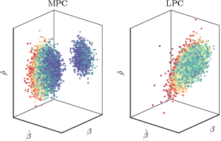
Altering the initial position of the target to $(1000,1500)$ m, and preserving all other parameters, we obtain roughly identical Gaussian distributions for MPC and LPC in Fig. 2. Full details for both Figs. 2 and 1 are given in Appendix A-2.

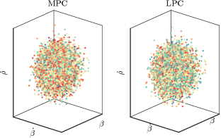
Our goal in investigating the post-manoeuvre distribution is to assess the viability of Kalman Filter approaches to target tracking. Such approaches work by estimating the target mean and covariance. Our concern is that those estimates can be inadequate or misleading if the underlying distribution has, for example, significant kurtosis. Proposition 2 establishes some special cases in which we do understand the distribution, but Figs. 1 and 2 demonstrate that, in the general case, the LPC post-manoeuvre distribution both can, and can not, resemble a Gaussian distribution. In order to assuredly use a Kalman Filter in LPC in the general case, we need to know whether a Gaussian approximation is defensible. For this reason, the main body of the paper derives the moments of the post-manoeuvre distribution. The skew and kurtosis of the post-manoeuvre distribution allow monitoring whether a Kalman Filter estimate can be trusted.

III-B Mean and Covariance of the Post-Manoeuvre Distribution

Define the pre-manoeuvre mean and covariance of the target state vector as $\bm{\mu}_{x}$ and $\Sigma_{x}$ ; we seek the corresponding post-manoeuvre mean and covariance, $\bm{\mu}^{+}_{x}$ and $\Sigma^{+}_{x}$ .

From Eq. 12, observe that any post-manoeuvre state space variable $x_{k}^{+}$ , where $k\in\{0,1,2,3\}$ , is defined in terms of its pre-manoeuvre value, bearing, and range as

x_{k}^{+}(x_{k})=x_{k}+a_{k}\frac{\sin\beta}{r}+b_{k}\frac{\cos\beta}{r},

(15)

where $a_{0}=a_{3}=b_{0}=b_{3}=0$ , $a_{1}=\Delta v_{y}$ and $b_{1}=-\Delta v_{x}$ , $a_{2}=-\Delta v_{x}$ and $b_{2}=-\Delta v_{y}$ .

The following results present the exact mean and covariance for the post-manoeuvre distribution.

Theorem 1 (Mean of the post-manoeuvre distribution).

The expected value of a post-manoeuvre variable $x_{k}^{+}$ defined in Eq. 15 is:

	$\displaystyle\mathbb{E}\left[x_{k}^{+}\right]=\;$	$\displaystyle\mathbb{E}\left[x_{k}\right]+e^{-\mu_{\rho}-\frac{1}{2}(\sigma_{\beta\beta}-\sigma_{\rho\rho})}(a_{k}\sin(\mu_{\beta}-\sigma_{\beta\rho})$
		$\displaystyle+b_{k}\cos(\mu_{\beta}-\sigma_{\beta\rho})).$		(16)

Proof.

The integrals for the mean values take the form

\mathbb{E}\left[x_{k}^{+}\right]=\int x_{k}^{+}(\bm{x})\mathcal{N}(\bm{x};\bm{\mu},\Sigma)d\bm{x}.

(17)

For $k\in\{0,3\}$ (bearing and log-range), $x_{k}^{+}=x_{k}$ , hence $\mathbb{E}\left[x^{+}_{k}\right]=\mu_{k}$ .

Now consider the mean for bearing rate, $k=1$ . Substituting Eq. 9 for $\dot{\beta}^{+}$ into Eq. 17, we get

$\displaystyle\mathbb{E}\left[\dot{\beta}^{+}\right]$	$\displaystyle=\int\dot{\beta}^{+}\mathcal{N}\!\left(\bm{x};\bm{\mu},\Sigma\right)d\bm{x}$
	$\displaystyle=\int\left(\dot{\beta}-\frac{\dot{\bm{w}}\cdot\bm{n}}{r}\right)\mathcal{N}\!\left(\bm{x};\bm{\mu},\Sigma\right)d\bm{x}$
	$\displaystyle=\mathbb{E}\left[\dot{\beta}\right]-\dot{\bm{w}}\cdot\mathbb{E}\left[\frac{\bm{n}}{r}\right].$	(18)

If we substitute the inverse range $r^{-1}$ with $e^{-\rho}$ and the sine and cosine components of $\bm{n}$ with real and imaginary parts of $e^{i\beta}$ , the last term becomes a linear combination of the real and imaginary parts of $\mathbb{E}\left[e^{-\rho+i\beta}\right]$ .

Note how this last expected value is similar to the moment-generating function (of the multivariate normal distribution), just for a complex-valued argument. As the case of a complex argument appears unnamed in the literature, we use the phrase ‘Generalised Gaussian MGF’.

Proposition 3 (The ‘Generalised Gaussian MGF’ (GGMGF)).

Let $\bm{h}\in\mathbb{C}^{n}$ be fixed and $\bm{x}\in\mathbb{R}^{n}$ be a Gaussian random variable. Then

\mathbb{E}\left[e^{\bm{h}^{\text{T}}\bm{x}}\right]=e^{\bm{\mu}^{\text{T}}\bm{h}+\frac{1}{2}\bm{h}^{\text{T}}\Sigma\bm{h}}\text{.}

(19)

This generalises the Gaussian moment-generating function (MGF) to complex arguments. The proof is described in §1.2 of [9] and §2 of [10].

Corollary 1 (GGMGF for specific $\bm{h}$ ).

For any $\bm{h}=[in,0,0,-m]$ , where $m,n\in\mathbb{N}\cup\{0\}$ , the GGMGF has the form

\!\!\mathbb{E}\!\left[r^{-m}e^{in\beta}\right]=e^{-m\mu_{\rho}-\frac{1}{2}\left(n^{2}\sigma_{\beta\beta}-m^{2}\sigma_{\rho\rho}\right)+i(n\mu_{\beta}-mn\sigma_{\beta\rho})}.

(20)

The real and imaginary parts of Eq. 20 give $\mathbb{E}\left[r^{-m}\cos\!{(n\beta)}\right]$ and $\mathbb{E}\left[r^{-m}\sin\!{(n\beta)}\right]$ , respectively.

Now, continuing the proof, to obtain the expected value of $e^{-\rho+i\beta}$ , we use Corollary 1 with $\bm{h}=[i,0,0,-1]$ to find

\!\mathbb{E}\!\left[e^{-\rho+i\beta}\right]=\exp{\!\big{(}\!-\mu_{\rho}-\frac{\sigma_{\beta\beta}-\sigma_{\rho\rho}}{2}+i(\mu_{\beta}-\sigma_{\beta\rho})\big{)}}.

(21)

The respective real and imaginary parts are $\mathbb{E}\left[r^{-1}\cos\beta\right]$ and $\mathbb{E}\left[r^{-1}\sin\beta\right]$ . Substitution of these expressions into Section III-B produces the mean of the post-manoeuvre bearing rate:

\mathbb{E}\!\left[\dot{\beta}^{+}\right]=\mathbb{E}\!\left[\dot{\beta}\right]-\left(\Delta v_{x}\cos(\mu_{\beta}-\sigma_{\beta\rho})\right.-\\ \left.\Delta v_{y}\sin(\mu_{\beta}-\sigma_{\beta\rho})\right)e^{-\mu_{\rho}-\frac{1}{2}(\sigma_{\beta\beta}-\sigma_{\rho\rho})}.

(22)

We can further simplify Eq. 22 by describing the ownship change in velocity through the turning angle $\alpha$ . Then, $\Delta v_{x}=\Delta v\cos\alpha$ and $\Delta v_{y}=\Delta v\sin\alpha$ , so that

\!\!\mathbb{E}\!\left[\dot{\beta}^{+}\right]\!=\mathbb{E}\!\left[\dot{\beta}\right]-\Delta ve^{-\mu_{\rho}-\frac{\sigma_{\beta\beta}-\sigma_{\rho\rho}}{2}}\cos{(\alpha+\mu_{\beta}-\sigma_{\beta\rho})}.

(23)

Finally, consider scaled range rate, $k=2$ . Using Eq. 9 for $\dot{\rho}^{+}$ in Eq. 17, and again employing Proposition 3, we obtain

$\displaystyle\mathbb{E}\!\left[\dot{\rho}^{+}\right]$	$\displaystyle=\int\dot{\rho}^{+}\mathcal{N}\!\left(\bm{x};\bm{\mu},\Sigma\right)d\bm{x}$
	$\displaystyle=\int\left(\dot{\rho}-s(\dot{\bm{w}}\cdot\bm{q})\right)\mathcal{N}\!\left(\bm{x};\bm{\mu},\Sigma\right)d\bm{x}$
	$\displaystyle=\mathbb{E}\left[\dot{\rho}\right]-\dot{\bm{w}}\cdot\mathbb{E}\left[e^{-\rho}\bm{q}\right]$
	$\displaystyle=\mathbb{E}\left[\dot{\rho}\right]-\left(\Delta v_{x}\sin(\mu_{\beta}-\sigma_{\beta\rho})\right.$
	$\displaystyle\quad\quad\left.+\Delta v_{y}\cos(\mu_{\beta}-\sigma_{\beta\rho})\right)e^{-\mu_{\rho}-\frac{1}{2}(\sigma_{\beta\beta}-\sigma_{\rho\rho})}$	(24)
	$\displaystyle=\mathbb{E}\left[\dot{\rho}\right]-\Delta ve^{-\mu_{\rho}-\frac{1}{2}(\sigma_{\beta\beta}-\sigma_{\rho\rho})}\sin{(\alpha+\mu_{\beta}-\sigma_{\beta\rho})}.$

Equations 22 and 24 match Theorem 1 with the coefficients $a_{k}$ and $b_{k}$ from Eq. 15, thus completing the proof. ∎

Now derive the second raw moments for the post-manoeuvre distribution. By combining these second raw moments with the first raw moments 1, we will also obtain the post-manoeuvre covariance matrix $\Sigma^{+}$ .

Theorem 2 (Second raw moment of the post-manoeuvre distribution).

For any two post-manoeuvre state space variables $x_{j}^{+}$ and $x_{k}^{+}$ , their second raw moment is:

$\displaystyle\mathbb{E}\!\left[x_{j}^{+}x_{k}^{+}\right]=\;$	$\displaystyle\mathbb{E}\left[x_{j}x_{k}\right]+a_{k}\mathbb{E}\!\left[x_{j}\frac{\sin{\beta}}{r}\right]+b_{k}\mathbb{E}\!\left[x_{j}\frac{\cos{\beta}}{r}\right]$
	$\displaystyle+a_{j}\mathbb{E}\!\left[x_{k}\frac{\sin{\beta}}{r}\right]+b_{j}\mathbb{E}\!\left[x_{j}\frac{\cos{\beta}}{r}\right]$
	$\displaystyle+\frac{a_{j}a_{k}+b_{j}b_{k}}{2}\mathbb{E}\!\left[\frac{1}{r^{2}}\right]$
	$\displaystyle+\frac{b_{j}b_{k}-a_{j}a_{k}}{2}\mathbb{E}\!\left[\frac{\cos{\!(2\beta)}}{r^{2}}\right]$
	$\displaystyle+\frac{a_{j}b_{k}+a_{k}b_{j}}{2}\mathbb{E}\!\left[\frac{\sin{\!(2\beta)}}{r^{2}}\right].$	(25)

All the expected values in this expression can be obtained in closed form using the GGMGF 19.

Corollary 2 ( $k=j$ case of second raw moment).

If $k=j$ for the two state space variables in Theorem 2, then

$\displaystyle\mathbb{E}\!\left[\left(x_{j}^{+}\right)^{2}\right]=\;$	$\displaystyle\mathbb{E}\!\left[x_{j}^{2}\right]+2a_{j}\mathbb{E}\!\left[x_{j}\frac{\sin{\beta}}{r}\right]+2b_{j}\mathbb{E}\!\left[x_{j}\frac{\cos{\beta}}{r}\right]$
	$\displaystyle+\frac{a_{j}^{2}+b_{j}^{2}}{2}\mathbb{E}\!\left[\frac{1}{r^{2}}\right]+\frac{b_{j}^{2}-a_{j}^{2}}{2}\mathbb{E}\!\left[\frac{\cos{\!(2\beta)}}{r^{2}}\right]$
	$\displaystyle+a_{j}b_{j}\mathbb{E}\!\left[\frac{\sin{\!(2\beta)}}{r^{2}}\right].$	(26)

Before presenting the proof of Theorem 2, we need one more auxiliary result. The theorem proof follows.

Lemma 1 (First derivative of GGMGF for specific $\bm{h}$ ).

For any $\bm{h}=[in,0,0,-m]$ , where $m,n\in\mathbb{N}\cup\{0\}$ , the first derivative of the GGMGF with respect to $x_{j}$ has the form

\mathbb{E}\left[x_{j}r^{-m}e^{in\beta}\right]=(\mu_{j}-m\sigma_{\rho j}+in\sigma_{\beta j})\mathbb{E}\left[r^{-m}e^{in\beta}\right].

(27)

Proof.

Consider the partial derivative of the GGMGF with respect to $h_{j}$ . Swapping the order of expectation and differentiation, we have

	$\displaystyle\mathbb{E}\left[x_{j}e^{\bm{h}^{\text{T}}\bm{x}}\right]$	$\displaystyle=\frac{\partial}{\partial h_{j}}\left(\mathbb{E}\left[e^{\bm{h}^{\text{T}}\bm{x}}\right]\right)$
		$\displaystyle=\frac{\partial}{\partial h_{j}}e^{\bm{\mu}^{\text{T}}\bm{h}+\frac{1}{2}\bm{h}^{\text{T}}\Sigma\bm{h}}$
		$\displaystyle=\left(\mu_{j}+\Sigma_{j}\bm{h}\right)e^{\bm{\mu}^{\text{T}}\bm{h}+\frac{1}{2}\bm{h}^{\text{T}}\Sigma\bm{h}},$

where $\Sigma_{j}$ denotes the $j^{\text{th}}$ row of the matrix $\Sigma$ . Without loss of generality, substitute $\bm{h}=[in,0,0,-m]$ into this expression to obtain Eq. 27. ∎

Proof of Theorem 2.

In the integral form, the second-order raw moments of the post-manoeuvre distribution are

\mathbb{E}\!\left[x_{j}^{+}x_{k}^{+}\right]=\int x_{j}^{+}x_{k}^{+}\mathcal{N}\!\left(\bm{x};\bm{\mu},\Sigma\right)d\bm{x}.

(28)

Substituting Eq. 15 for $x_{j}^{+}$ , $x_{k}^{+}$ , expanding the product, then interchanging the order of integration and expectation, and grouping the terms with the same expected values we obtain the decomposition 2. All the expected values in Theorem 2 are given in closed form by the real and imaginary parts of Eqs. 20 and 27 for the respective $m$ and $n$ indices. ∎

Corollary 2 immediately follows from Theorem 2 for $j=k$ . Therefore, we have derived closed-form expressions for all the post-manoeuvre first and second (raw and central) moments.

III-C Higher-Order Moments of the Post-Manoeuvre Distribution

In Theorems 1 and 2, we see that the first two moments of the post-manoeuvre distribution are linear combinations of pre-manoeuvre moments. We generalise this for the arbitrary $N^{\text{th}}$ raw moment of the post-manoeuvre distribution.

Proposition 4 ( $N^{\text{th}}$ raw moment of the post-manoeuvre distribution).

For post-manoeuvre state space variables $x_{k}^{+}$ each raised to powers $q_{k}$ , $k=0,\dots,3$ , such that $\sum_{j=0}^{3}q_{k}=N$ , the $N^{\text{th}}$ raw moment is

\displaystyle\!\!\!\mathbb{E}\!\left[\prod_{k=0}^{3}(x_{k}^{+})^{q_{k}}\right]\!=\mathbb{E}\!\left[\prod_{k=0}^{3}\!\left(x_{k}+a_{k}\frac{\sin\beta}{r}+b_{k}\frac{\cos\beta}{r}\!\right)^{q_{k}}\right]\!\!,

(29)

which, when expanded, yields a linear combination of

	$\displaystyle E_{p_{0},p_{1},p_{2},p_{3},m,n}^{(s)}$	$\displaystyle=\mathbb{E}\left[\prod_{k=0}^{3}x_{k}^{p_{k}}r^{-m}\sin(n\beta)\right]\text{, and}$
	$\displaystyle E_{p_{0},p_{1},p_{2},p_{3},m,n}^{(c)}$	$\displaystyle=\mathbb{E}\left[\prod_{k=0}^{3}x_{k}^{p_{k}}r^{-m}\cos(n\beta)\right],$		(30)

where $\sum_{k=0}^{3}p_{k}+m=N$ , for $0\leq n\leq m$ .

Proof.

Consider the product

\prod_{k=0}^{3}\left(x_{k}+a_{k}\frac{\sin\beta}{r}+b_{k}\frac{\cos\beta}{r}\right)^{q_{k}}

from the right-hand side of Eq. 29. Expansion via the binomial theorem yields a linear combination of terms

\prod_{k=0}^{3}x_{k}^{p_{k}}r^{-(c+d)}\sin^{c}{\beta}\cos^{d}{\beta},

(31)

where $\sum_{k=0}^{3}p_{k}+c+d=N$ .

Using De Moivre’s formula, Euler’s formula, and the binomial theorem, we convert the powers $\sin^{c}{\beta}$ and $\cos^{d}{\beta}$ to sums of $\sin(c^{*}\beta)$ and $\cos(d^{*}\beta)$ , where $c^{*}=0,\dots,c$ and $d^{*}=0,\dots,d$ . Expanding again the product of these sums, and using the trigonometric addition identities, each element 31 becomes a linear combination of terms

\prod_{k=0}^{3}x_{k}^{p_{k}}r^{-m}\sin\!{(n\beta)},\quad\prod_{k=0}^{3}x_{k}^{p_{k}}r^{-m}\cos\!{(n\beta)},

(32)

where $m=c+d$ , $\sum_{k=0}^{3}p_{k}+m=N$ , and $0\leq n\leq m$ .

Therefore, using the linearity of expectation, the right-hand side of Eq. 29 is a linear combination of $E_{p_{0},p_{1},p_{2},p_{3},m,n}^{(s)}$ and $E_{p_{0},p_{1},p_{2},p_{3},m,n}^{(c)}$ defined in Proposition 4, which are the expected values of expressions 32. ∎

The expected values in Proposition 4 can be found in closed form by recursive application of the following Lemma.

Lemma 2 ( $N^{\text{th}}$ partial derivative of the GMGF).

The $N^{\text{th}}$ partial derivative of the GMGF, conditioned by $\sum_{k=0}^{3}p_{k}+m=N$ , $p_{j}\geq 0$ , and $m\geq 0$ , is


$\displaystyle\mathbb{E}\left[e^{\bm{h}^{\text{T}}\bm{x}}\prod_{k=0}^{3}x_{k}^{p_{k}}\right]=$	$\displaystyle\frac{\partial^{N}\Phi_{\bm{x}}(\bm{h})}{\partial h_{j}^{p_{j}}\partial h_{k}^{p_{k}}\dots}$
$\displaystyle=$	$\displaystyle\sum_{j\neq k}p_{j}\sigma_{jk}\frac{\partial^{N-2}\Phi_{\bm{x}}(\bm{h})}{\partial h_{j}^{p_{j}-1}\partial h_{k}^{p_{k}-1}\dots}$	(33a)
	$\displaystyle+(p_{k}-1)\sigma_{kk}\frac{\partial^{N-2}\Phi_{\bm{x}}(\bm{h})}{\partial h_{j}^{p_{j}}\partial h_{k}^{p_{k}-2}\dots}$	(33b)
	$\displaystyle+\left(\mu_{k}+\Sigma_{k}\bm{h}\right)\frac{\partial^{N-1}\Phi_{\bm{x}}(\bm{h})}{\partial h_{j}^{p_{j}}\partial h_{k}^{p_{k}-1}\dots},$	(33c)

where $k$ is selected such that $p_{k}>1$ , which is always possible for $N\geq 1$ . The index $k$ is not specific, any index can be selected due to the symmetry of derivatives.

For the sake of brevity, the notation in Eq. 33 technically allows negative derivatives of order $-1$ if $p_{j}=0$ for some elements in Eq. 33a, or if $p_{k}=1$ in Eq. 33b. However, such terms are eliminated by the corresponding $p_{j}=0$ and $p_{k}-1$ multipliers in front.

Proof.

For $N=1$ , we re-write Eq. 27 as

\frac{\partial}{\partial h_{k}}\Phi_{\bm{x}}(\bm{h})=\left(\mu_{k}+\Sigma_{k}\bm{h}\right)\Phi_{\bm{x}}(\bm{h}).

(34)

For $N=2$ , we take the second partial derivative to obtain

$\displaystyle\frac{\partial^{2}}{\partial h_{k}\partial h_{j}}\Phi_{\bm{x}}(\bm{h})$	$\displaystyle=\frac{\partial}{\partial h_{k}}\left(\mu_{j}+\Sigma_{j}\bm{h}\right)\Phi_{\bm{x}}(\bm{h})$
	$\displaystyle=\bigl{(}\sigma_{jk}+\left(\mu_{j}+\Sigma_{j}\bm{h}\right)\left(\mu_{k}+\Sigma_{k}\bm{h}\right)\bigr{)}\Phi_{\bm{x}}(\bm{h})$
	$\displaystyle=\leavevmode\resizebox{258.36667pt}{}{$\sigma_{jk}\Phi_{\bm{x}}(\bm{h})+\left(\mu_{k}+\Sigma_{k}\bm{h}\right)\frac{\partial}{\partial h_{j}}\Phi_{\bm{x}}(\bm{h})$}.$	(35)

These expressions start the recursion of Eq. 33: for $j\neq k$ , the first term of Section III-C yields Eq. 33a, and for $j=k$ , it yields Eq. 33b. Eq. 34 and the last term of Section III-C produce Eq. 33c for the respective $N=1,2$ .

The proof for a general order $N$ is obtained through direct differentiation of Eq. 33 by $h_{m}$ for some arbitrary $m$ : the partial derivatives in Eqs. 33a to 33c increase the order of their $h_{m}$ -th derivatives by one. Then the derivative of the $\mu_{k}+\Sigma_{k}\bm{h}$ term in Eq. 33c yields one more summand with a $\sigma_{km}$ multiplier. If $k\neq m$ , it is combined with the corresponding $j=m$ term of Eq. 33a to increase its $p_{m}$ multiplier in front to $p^{\prime}_{m}=p_{m}+1$ . Alternatively, for $k=m$ the new summand is combined with Eq. 33b to increase the $p_{k}-1=p_{m}-1$ multiplier to $p_{m}=p^{\prime}_{m}-1$ . In both cases, we obtain Eq. 33 with substitutions $N\Rightarrow N^{\prime}=N+1$ and $p_{m}\Rightarrow p^{\prime}_{m}=p_{m}+1$ , which is the next order of recursion. ∎

Substituting $\bm{h}=[in,0,0,-m]$ into Eq. 33 recursively yields the expected values from Proposition 4.

By Proposition 4, any $N^{\text{th}}$ order raw moment is

	$\displaystyle\mathbb{E}\left[\prod_{k=0}^{3}(x_{k}^{+})^{q_{k}}\right]$	$\displaystyle=\sum_{\{q,m\}}\sum_{n=0}^{m}\left(S_{p_{0},\dots,p_{3},m,n}^{(p_{0},\dots,p_{3})}E_{p_{0},\dots,p_{3},m,n}^{(s)}\right.$
		$\displaystyle\left.+C_{p_{0},\dots,p_{3},m,n}^{(p_{0},\dots,p_{3})}E_{p_{0},\dots,p_{3},m,n}^{(c)}\right).$		(36)

The first sum considers all possible combinations of $p_{k}$ , $k=0,\dots,3$ and $m$ subject to the conditions $\sum_{k=0}^{3}p_{k}+m=N$ , $p_{k}\geq 0$ , $m\geq 0$ . The coefficients $S_{p_{0},\dots,p_{3},m,n}^{(p_{0},\dots,p_{3})}$ and $C_{p_{0},\dots,p_{3},m,n}^{(p_{0},\dots,p_{3})}$ are products of $a_{k}$ and $b_{k}$ and can be found from Eqs. 29 and 15.

We demonstrated that any higher-order moment of the post-manoeuvre distribution can be found in closed form by recursive application of Eqs. 33 and III-C. However, as the order of the moment increases, so does the complexity of its closed-form expression. Explicit calculation of the coefficients $S_{p_{0},\dots,p_{3},m,n}^{(p_{0}^{+},\dots,p_{3}^{+})}$ and $C_{p_{0},\dots,p_{3},m,n}^{(p_{0}^{+},\dots,p_{3}^{+})}$ quickly becomes prohibitive. Combined with the non-Gaussianity proven in Section III-A, such that we have no existing statistical results to draw on, we turn to computer algebra for deriving specific cases of Section III-C. We have developed a package in SageMath [11] to generate these moments and export them as LaTeX or Python code. A demonstration of this package is shown in Appendix B.

The first two moments are explicitly given by Theorems 1 and 2. In the next section, we apply these two moments in a modified UKF estimator, while using the higher-order moments to monitor its performance.

IV Applications of the Closed-Form Expressions in Tracking Simulation

IV-A UKF using Closed-Form Expressions for Mean and Covariance Prediction

The Kalman Filter provides a minimum square error estimate for the mean and covariance of the target location [12]. For our non-linear dynamical system, the UKF is appropriate. It uses the UT to propagate deterministic sigma points that accurately capture the target state mean and covariance [7].

In order to test our closed-form expressions in tracking simulation, we will implement a pure UKF and a modified UKF that incorporates our closed-form expressions. We assume the ownship alternates between straight legs and instant turns. The modified UKF employs the first two moments of the post-manoeuvre distribution to calculate the target state and covariance after each ownship turn.

We define the ownship manoeuvre at time step $i$ as a tuple of three values:

•

$\Delta\bm{r}_{i}$ , the accelerated displacement during the step illustrated in Fig. 3.
•

$\Delta\bm{v}_{i}$ , the speed change during the step; the speed changes instantly at the point of the turn, at unknown time within the step.
•

$\Delta t_{i}$ , the time duration of the step.

As the turn may happen at a time instance within the step, we seek to split the manoeuvre into elementary movements, or sub-manoeuvres: a straight leg, an instant turn, and another straight leg after the turn. The duration of the two straight legs adds up to the total duration of the time step $\Delta t_{i}$ . Computation of these sub-manoeuvres is described in Theorem 3.

Figure 3: A diagram of the predicted ownship position,

\bm{r}_{1}^{\prime}

, versus the true position,

\bm{r}_{3}

, where the black node indicates the point of the instant turn. Note the jump from index

1

3

as the second sub-manoeuvre, the instant turn, has zero duration, zero accelerated displacement (hence, zero length on the plot), but non-zero change in velocity:

\Delta\bm{v}=\bm{v}_{3}-\bm{v}_{1}

. The accelerated displacement is

\Delta\bm{r}=\bm{r}_{3}-\bm{r}_{1}^{\prime}

Theorem 3 (Manoeuvre splitting).

The manoeuvre containing a turn $M(\Delta\bm{r},\Delta\bm{v},\Delta t)$ is equivalently described as a list of three sub-manoeuvres:

1.

$M_{1}(0,0,\Delta t_{1})$ ,
2.

$M_{2}(0,\Delta\bm{v},0)$ , and
3.

$M_{3}(0,0,\Delta t_{3})$

where

\Delta t_{3}=\frac{\Delta\bm{r}\cdot\Delta\bm{v}}{|\Delta\bm{v}|^{2}}

(37)

and $\Delta t_{1}=\Delta t-\Delta t_{3}$ .

Proof.

We write the final position in terms of the initial position and two velocities.

\bm{r}_{3}=\bm{r}_{1}+\Delta t_{1}\bm{v}_{1}+\Delta t_{3}\bm{v}_{3}.

Substituting $\Delta t_{3}=\Delta t-\Delta t_{1}$ and regrouping, we get

\bm{r}_{3}-(\bm{r}_{1}+\Delta t\bm{v}_{1})=\Delta t_{3}(\bm{v}_{3}-\bm{v}_{1}).

As illustrated in Fig. 3, the left-hand side is the accelerated displacement $\Delta\bm{r}$ ; the term in brackets in the right-hand side is the speed change $\Delta\bm{v}$ . Therefore,

\Delta\bm{r}=\Delta t_{3}\Delta\bm{v}.

By assumption of a non-zero turn, $|\Delta\bm{v}|\neq 0$ . Thus, multiplying both sides by $\Delta\bm{v}$ we obtain Eq. 37. ∎

In cases where the turn is at the start or at the end of the total manoeuvre, without loss of generality, we split the total manoeuvre into two: a turn and a straight leg.

Having established the approach for isolating instant turns, we present the modified filter, CFE-UKF, as Algorithm 1.

Algorithm 1 The modified UKF algorithm, CFE-UKF, that uses the closed-form expressions 1 and 2 to update the mean and covariance over instant turns.

1:function CFE-UKF

2: Initialise at time

t_{0}

, iteration

0

N_{T}

is the total count of time steps

4: for

i\in[1,N_{T}]

5: Advance platforms forward by time step

\Delta t_{i}

6: Compute the manoeuvre

M_{i}(\Delta\bm{r}_{i},\Delta\bm{v}_{i},\Delta t_{i})

7: if

|\Delta\bm{v}_{i}|<\epsilon

then

\triangleright

no turn

8: Time update over

\Delta t_{i}

using UT

9: else

10: Split

M_{i}

into sub-manoeuvres

[M_{j}]

11: for all

M_{j}\in[M_{j}]\ \textbf{do}

12: if

\Delta\bm{v}_{j}\neq\bm{0}

then

\triangleright

ownship turned

13: State update by Theorems 1 and 2

14: else

\triangleright

straight leg

15: Time update over

\Delta t_{j}

using UT

16: end if

17: end for

18: end if

19: Measurement update of the UKF as usual

20: end for

21:end function

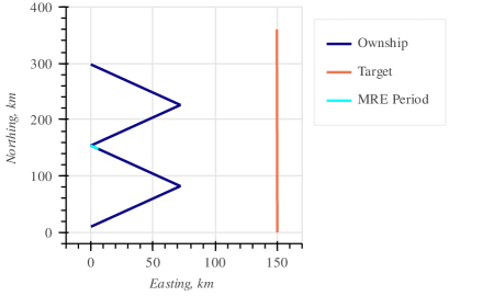
To compare the CFE-UKF with a pure UKF, we use a scenario presented in Fig. 4. The ownship moves deterministically along straight lines, and makes exact turns, while the target movement is subject to the process noise provided by the continuous-time white noise model with nearly constant velocity [13]. The time increment $\Delta t$ is 10 seconds.

For the purposes of verification, we first run the CFE-UKF and UKF with artificially precise parameters. The process noise intensity is set to $10^{-8}$ and the sensor standard deviation of bearing measurements to 0.001°. We set the initial track range to $150$ km (the true range from ownship to target) and initialise the range variance to $10$ % of the true range. In this idealised case, we find both trackers run very similarly: the averaged absolute difference between their means is only $[1.3\cdot 10^{-9},1.8\cdot 10^{-11},3.9\cdot 10^{-10},1.8\cdot 10^{-5}]$ .

The CFE-UKF is slightly less efficient than a pure UKF; for each turning point, we perform up to two UTs, depending on whether there is a preceding and succeeding straight leg, and then additionally compute the closed-form expressions to update the mean and covariance over the turn. However, due to our small state space dimension $n_{x}=4$ , and the small proportion of ownship turns relative to the total scenario, this increase in complexity has minimal effect on total run-time.

IV-B Monitoring Gaussianity Using the Third and Fourth Central Moments of the Post-Manoeuvre Distribution

In Section III-A we have shown that the post-manoeuvre distribution is not Gaussian. Now we can quantify this statement. When the ownship turns, we know the higher-order moments of the post-manoeuvre state distribution, and can use them to monitor how close is this distribution to Gaussian. The turning points are critical for passive BO tracking because only there the range becomes observable, and therefore, it is vital for the estimator assumptions, e.g. Gaussianity, to be satisfied.

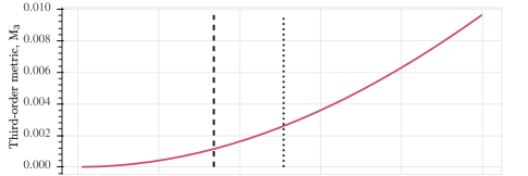
We consider two metrics for use as a monitoring tool. The first it is the Frobenius norm of the third central moment tensor

M_{3}=\big{\lVert}\,\mathbb{E}\left[(\bm{x}^{+}-\bm{\mu}^{+})^{3}\right]\!\big{\rVert}.

(38)

For a Gaussian distribution $M_{3}\equiv 0$ , hence a non-zero value is a measure of non-Gaussianity.

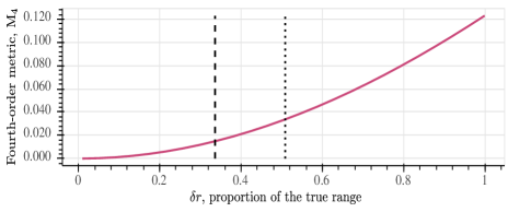
The second metric is the norm of the deviation of the post-manoeuvre fourth central moment, a $4^{\text{th}}$ -order tensor, from the expected fourth central moment of a Gaussian distribution:

M_{4}=\big{\lVert}\,\mathbb{E}\!\left[(\bm{x}^{+}-\bm{\mu}^{+})^{4}\right]-\mathbb{E}\!\left[(\bm{y}-\bm{\mu}^{+})^{4}\right]\!\big{\rVert},

(39)

where $y\sim\mathcal{N}(\bm{\mu}^{+},\Sigma^{+})$ . Again, $M_{4}\equiv 0$ for a Gaussian distribution; a non-zero value quantifies non-Gaussianity.

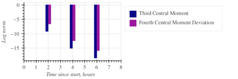
Figure 5 shows the time series of the proposed metrics for the scenario of Fig. 4. To make the simulations somewhat less idealised, from now on the process noise intensity is increased to $10^{-6}$ and the bearing measurement error to 0.1°. Clearly, the distribution is not Gaussian when the ownship turns. On the positive side, we observe that with every subsequent turn the metrics decrease, implying that the distribution becomes more Gaussian with time as the estimators converge. Consequently, it may imply that the observed non-Gaussianity is related to the estimator initialisation, and that is what we examine next.

IV-C Effect of Range Error Initialisation on the Post-Manoeuvre Distribution

To start the estimator, we need to provide the initial state $\bm{x}_{0}$ and covariance $\Sigma_{0}$ . In the examples presented in this paper, we set $\bm{x}_{0}$ using the first meaured bearing for $\beta_{0}$ , zeros for the derivatives $\dot{\beta}_{0}$ and $\dot{\rho}_{0}$ , and the true value for the initial range $r_{0}$ . The covariance $\Sigma_{0}$ is set to a diagonal matrix of

•

the sensor measurement variance for bearing,
•

${(v_{\text{max}}/r_{0})}^{2}$ for the bearing and scaled range rates, where $v_{\text{max}}$ is some “large” speed value, and
•

$\sigma_{rr}=\log{(1+{(\delta r)}^{2})}$ for log-range, were we introduce $\delta r$ as the initial relative range error.

We express the log-range error in terms of $\delta r$ , because in the limit of small errors, the range variance of ${(r_{0}\delta r)}^{2}$ indeed corresponds to the log-range variance of $\sigma_{rr}$ . For larger errors the relationship breaks down, but $\delta r$ still provides a convenient description of the error in human terms, as opposed to the less intuitive variance of the range logarithm.

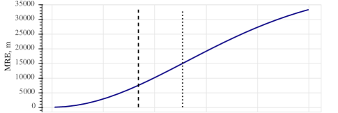
To examine the impact of initialisation on the tracking accuracy and on the properties of the post-manoeuvre distribution, we consider the estimator output after the first manoeuvre of our scenario, where the non-Gaussianity is most pronounced. As a measure of accuracy, we use the mean estimated range error (MRE) calculated over ten minutes of the scenario at the end of the second leg (highlighted in Fig. 4 with cyan).

The dependence of the MRE on tracker initialisation is presented in Fig. 6. The corresponding two metrics of target state Gaussianity after the first ownship turn are shown in Figs. 6 and 6. As expected, estimation error grows with initialisation ambiguity. Correspondingly, the post-manoeuvre state distribution becomes less Gaussian, thus violating the UKF assumptions and reducing estimator accuracy.

A corollary of the presented result is that monitoring non-Gaussianity enables a measure of control of the estimator performance. This is the motivation for the CFE-UKF. While it may not perform that differently from the pure UKF, the new estimator provides the user with a capability to monitor whether the underlying assumptions of the Gaussian estimator are being met.

Whenever the non-Gaussianity metrics exceed certain thresholds²²2 The specific thresholds for $M_{3}$ and $M_{4}$ metrics can be established by Monte-Carlo modelling, but are beyond the scope of this paper., the user would know that the target range estimate after the manoeuvre cannot be trusted, even if the estimated range variance is low. In such a case, the ownship may, for example, attempt the next manoeuvre to improve the solution. Figure 5 shows how Gaussianity of the post-manoeuvre distribution improves on each turn, thus validating the estimator convergence. Alternatively, the same Gaussianity metrics can guide the choice of the initial range variance $\delta r$ .

The focus of this section has been the use of our results in a Kalman Filter framework. One may consider more powerful filtering algorithms that do not assume Gaussianity of the target state; these are discussed in the next section.

V Conclusions and Future Work

The paper extends the theoretical understanding of object tracking in LPC. In order to make the theory tractable, we assume an instantaneous manoeuvre and a target moving in a straight line. Under these simplifications, we obtain some strong results. The main contribution of the paper is Proposition 4: we derive all moments of the post-manoeuvre distribution in closed form. Additionally, Proposition 2 derives, for both LPC and MPC, special cases in which the post-manoeuvre distribution is Gaussian, with known parameters. Our results, while formally obtained for instantaneous manoeuvres, may be applied in the general, non-instantaneous case through discretisation.

As the contributions of the paper are primarily theoretical, let us now discuss possible applications of the theory. The most common class of tracking algorithms, consisting of extensions of the Kalman Filter for non-linear system dynamics, work best when the state distribution of the target is approximately unimodal and without large outliers. Our contribution allows a user to track the third and fourth moments of the LPC distribution, and thereby assess when these conditions are met.

We demonstrate the utility of the obtained results in filtering algorithms. For state and covariance prediction, we define a new algorithm, the CFE-UKF, that uses the closed-form expressions for mean and covariance in place of the UT-based time update over an instant ownship turn. By comparing with the well-understood UKF in a simple tracking scenario, we confirm our results for the first two moments of the post-manoeuvre distribution are correct. However, in addition to the mean and covariance, our estimator also computes the third and fourth post-manoeuvre moments to allow monitoring of the quality of the Gaussian approximation, an ability that the pure UKF lacks. This insight gives the CFE-UKF an edge over the UT-based estimator.

With this understanding, we conclude that there is a need to evaluate algorithms that do not blindly assume Gaussianity of the underlying target state distribution. Similar to the approaches presented in [14], we could use our higher-order moment metrics as splitting criteria for a Gaussian sum filter; a threshold established by Monte-Carlo modelling can determine when the estimator would benefit from a split of the prior when the ownship turns.

Alternatively, the conditional Gaussianity properties proved in Proposition 2 empower the use of a Rao-Blackwell-type particle filter; a particle filter would track the bearing rate and scaled range rate, while bearing and log-range are conditionally Gaussian and can be tracked with a Kalman Filter.

Acknowledgements

We thank Acacia Systems for their support and funding.

Appendix A Supplemental details for Section III-A

1. Proof of Proposition 2

Proof.

Claims (1)(i) and (2)(i), that the post-manoeuvre distributions of MPC and LPC are non-Gaussian, are clearly visible from the terms in $\cos\beta$ and $\sin\beta$ , which are entangled with $\dot{\beta}$ and $\dot{\rho}$ in the exponent of the post-manoeuvre distribution. Let $P_{i,j}$ refer to the $i,j^{\text{th}}$ entry of the precision matrix $\Sigma^{-1}$ ; then the exponent of Eq. 14 contains a term

(\dot{\rho}-\mu_{\rho}+s\Delta v_{x}\sin\beta+s\Delta v_{y}\cos\beta)^{2}P_{2,2}\;.

Expanding this quadratic reveals terms like, for example, $\dot{\rho}sP_{2,2}\sin\beta$ , that render the distribution non-Gaussian. One might wonder whether these terms can cancel with other terms in the distribution — but cancellation is impossible without requiring special conditions on the precision matrix entries.

Claim (1)(ii), that the MPC distribution is known exactly if we condition on the bearing $\beta$ , is proven as follows. As in the Proposition, let $c_{1}$ and $c_{2}$ refer to the constant factors in $f_{1}$ and $f_{2}$ . Accordingly, Eq. 10 in MPC becomes

\bm{h}^{-1}(\bm{x}^{+})=\begin{bmatrix}\beta^{+}\\ \dot{\beta}^{+}+c_{1}s^{+}\\ \dot{\rho}^{+}+c_{2}s^{+}\\ s^{+}\end{bmatrix}\;,

and on substitution into Eq. 14 and conditioning on $\beta$ , the exponent of the post-manoeuvre distribution is

-\frac{1}{2}\left[\left(\begin{bmatrix}\dot{\beta}^{+}+c_{1}s^{+}\\ \dot{\rho}^{+}+c_{2}s^{+}\\ s^{+}\end{bmatrix}-\bm{\mu}\right)^{{}^{\text{T}}}\Sigma^{-1}_{-\beta}\left(\begin{bmatrix}\dot{\beta}^{+}+c_{1}s^{+}\\ \dot{\rho}^{+}+c_{2}s^{+}\\ s^{+}\end{bmatrix}-\bm{\mu}\right)\right].

We now write the vectors that pre- and post-multiply $\Sigma$ as linear transformations of Gaussian innovations. Let $d_{3}=s^{+}-\mu_{s}$ , then

\dot{\beta}^{+}+c_{1}s^{+}-\mu_{\dot{\beta}}=\dot{\beta}-(\mu_{\dot{\beta}}-c_{1}\mu_{s})+c_{1}d_{3},

\dot{\rho}^{+}+c_{2}s^{+}-\mu_{\dot{\rho}}=\dot{\rho}-(\mu_{\dot{\rho}}-c_{2}\mu_{s})+c_{2}d_{3}.

Accordingly, let $d_{1}=\dot{\beta}-(\mu_{\dot{\beta}}-c_{1}\mu_{s})$ and $d_{2}=\dot{\rho}-(\mu_{\dot{\rho}}-c_{2}\mu_{s})$ , then the exponent simplifies to

-\frac{1}{2}\left[\begin{pmatrix}d_{1}+c_{1}d_{3}\\ d_{2}+c_{2}d_{3}\\ d_{3}\end{pmatrix}^{\text{T}}\Sigma^{-1}\begin{pmatrix}d_{1}+c_{1}d_{3}\\ d_{2}+c_{2}d_{3}\\ d_{3}\end{pmatrix}\right].

Clearly, the vectors are a linear combination of $d_{1},\,d_{2},\,d_{3}$ . Recalling the definition of $\mathbf{P}$ from the Proposition, we get

\begin{pmatrix}d_{1}+c_{1}d_{3}\\ d_{2}+c_{2}d_{3}\\ d_{3}\end{pmatrix}=\begin{pmatrix}1&0&c_{1}\\ 0&1&c_{2}\\ 0&0&1\end{pmatrix}\begin{pmatrix}d_{1}\\ d_{2}\\ d_{3}\end{pmatrix}=\mathbf{P}^{-1}\begin{pmatrix}d_{1}\\ d_{2}\\ d_{3}\end{pmatrix}

and simplify the exponent to

-\frac{1}{2}\left[\begin{pmatrix}d_{1}\\ d_{2}\\ d_{3}\end{pmatrix}^{\text{T}}\left(\mathbf{P}^{-1}\right)^{\text{T}}\Sigma^{-1}\mathbf{P}^{-1}\begin{pmatrix}d_{1}\\ d_{2}\\ d_{3}\end{pmatrix}\right]\;.

Recognising that $\left(\mathbf{P}^{-1}\right)^{\text{T}}\Sigma^{-1}\mathbf{P}^{-1}=\left(\mathbf{P}\Sigma\mathbf{P}^{\text{T}}\right)^{-1}$ , we conclude the stated result.

Claim (2)(ii), on the Gaussian distribution for LPC if conditioned on $\beta$ and $\rho$ , is trivial: simply recognise that the terms $f_{1}(\beta,\rho)$ and $f_{2}(\beta,\rho)$ are fixed and can be thought of as modifications to the means of $\dot{\beta}$ and $\dot{\rho}$ . ∎

2. Details of Figs. 1 and 2

Each Figure considers a Gaussian prior in MPC / LPC coordinates using a diagonal $\Sigma$ . The main challenge is to select the mean and variance for $s$ and $\rho$ so that the priors are roughly comparable between the two coordinate systems. In order to do so, we select an initial location for the target in Cartesian coordinates — $(0.1,0.15)$ km in Fig. 1 and $(1,1.5)$ km in Fig. 2 — and an initial standard deviation for target location uncertainty of $0.4$ km in Cartesian space. We sample 10,000 times from this Gaussian prior in Cartesian coordinates, transform each sample into $s$ and $\rho$ , and use the variance of the transformed samples as the variance of the prior in LPC / MPC. The resulting standard deviations, and all other parameters for the figures, are shown in Table I. The figures are then obtained by sampling 10,000 times from each prior and transforming those samples: label the $i^{\text{th}}$ sample $\bm{x}_{i}$ , then the figures plot $\bm{x}_{i}^{+}=\bm{h}(\bm{x}_{i})$ for all $i$ .

		$\mu_{\beta}$	$\mu_{\dot{\beta}}$	$\mu_{\dot{\rho}}$	$\mu_{s/\rho}$	$\sigma^{2}_{\beta}$	$\sigma^{2}_{\dot{\beta}}$	$\sigma^{2}_{\dot{\rho}}$	$\sigma^{2}_{s/\rho}$
Fig. 1	MPC	0.58	1.1	0.1	5.5	0.05	0.2	0.2	4.0
Fig. 1	LPC	0.58	1.1	0.1	-1.7	0.05	0.2	0.2	0.63
Fig. 2	MPC	0.58	1.1	0.1	0.55	0.05	0.2	0.2	0.14
Fig. 2	LPC	0.58	1.1	0.1	0.59	0.05	0.2	0.2	0.23

TABLE I: Means and variances for Gaussian priors, obtained as described in Appendix A.

Appendix B Demonstration of Higher-Order Moment Generation via Computer Algebra

Our SageMath package, seaweed \faGitSquare, exports any moment of the post-manoeuvre target state distribution as Python or LaTeX code. For example, we present the third raw moment of bearing rate in LaTeX in Appendix B. We have manually written the expected value on the left-hand side, but we directly obtain the right-hand side by calling the function moment_0300/latex_0300 in the pre-generated post_manoeuvre module.

There is a minor stylistic difference between the generated moments and the main body of this paper; the two components of ownship speed change, $\Delta v_{x}$ and $\Delta v_{y}$ , are respectively written as $\Delta v_{0}$ and $\Delta v_{1}$ . We have also manually added line breaks and alignment markers to fit the equation to the page.

$\displaystyle\mathbb{E}\!\left[x^{3}_{1}\right]=$	$\displaystyle-\frac{3}{4}\,$	$\displaystyle{\Delta v_{0}}^{3}\cos\left(\mu_{0}-3\,\sigma_{30}\right)e^{\left(-3\,\mu_{3}-\frac{1}{2}\,\sigma_{00}+\frac{9}{2}\,\sigma_{33}\right)}-\frac{3}{4}\,{\Delta v_{0}}{\Delta v_{1}}^{2}\cos\left(\mu_{0}-3\,\sigma_{30}\right)e^{\left(-3\,\mu_{3}-\frac{1}{2}\,\sigma_{00}+\frac{9}{2}\,\sigma_{33}\right)}$
	$\displaystyle-\frac{1}{4}\,$	$\displaystyle{\Delta v_{0}}^{3}\cos\left(3\,\mu_{0}-9\,\sigma_{30}\right)e^{\left(-3\,\mu_{3}-\frac{9}{2}\,\sigma_{00}+\frac{9}{2}\,\sigma_{33}\right)}+\frac{3}{4}\,{\Delta v_{0}}{\Delta v_{1}}^{2}\cos\left(3\,\mu_{0}-9\,\sigma_{30}\right)e^{\left(-3\,\mu_{3}-\frac{9}{2}\,\sigma_{00}+\frac{9}{2}\,\sigma_{33}\right)}$
	$\displaystyle+\frac{3}{4}\,$	$\displaystyle{\Delta v_{0}}^{2}{\Delta v_{1}}e^{\left(-3\,\mu_{3}-\frac{9}{2}\,\sigma_{00}+\frac{9}{2}\,\sigma_{33}\right)}\sin\left(3\,\mu_{0}-9\,\sigma_{30}\right)-\frac{1}{4}\,{\Delta v_{1}}^{3}e^{\left(-3\,\mu_{3}-\frac{9}{2}\,\sigma_{00}+\frac{9}{2}\,\sigma_{33}\right)}\sin\left(3\,\mu_{0}-9\,\sigma_{30}\right)$
	$\displaystyle+\frac{3}{4}\,$	$\displaystyle{\Delta v_{0}}^{2}{\Delta v_{1}}e^{\left(-3\,\mu_{3}-\frac{1}{2}\,\sigma_{00}+\frac{9}{2}\,\sigma_{33}\right)}\sin\left(\mu_{0}-3\,\sigma_{30}\right)+\frac{3}{4}\,{\Delta v_{1}}^{3}e^{\left(-3\,\mu_{3}-\frac{1}{2}\,\sigma_{00}+\frac{9}{2}\,\sigma_{33}\right)}\sin\left(\mu_{0}-3\,\sigma_{30}\right)$
	$\displaystyle+\frac{3}{2}\,$	$\displaystyle{\Delta v_{0}}^{2}{\left(\mu_{1}-2\,\sigma_{31}\right)}e^{\left(-2\,\mu_{3}+2\,\sigma_{33}\right)}+\frac{3}{2}\,{\Delta v_{1}}^{2}{\left(\mu_{1}-2\,\sigma_{31}\right)}e^{\left(-2\,\mu_{3}+2\,\sigma_{33}\right)}$
	$\displaystyle+\frac{3}{2}\,$	$\displaystyle{}{\left({\left(\mu_{1}-2\,\sigma_{31}\right)}\cos\left(2\,\mu_{0}-4\,\sigma_{30}\right)e^{\left(-2\,\mu_{3}-2\,\sigma_{00}+2\,\sigma_{33}\right)}-2\,\sigma_{10}e^{\left(-2\,\mu_{3}-2\,\sigma_{00}+2\,\sigma_{33}\right)}\sin\left(2\,\mu_{0}-4\,\sigma_{30}\right)\right)}{\Delta v_{0}}^{2}$
	$\displaystyle-3\,$	$\displaystyle{}{\left(2\,\sigma_{10}\cos\left(2\,\mu_{0}-4\,\sigma_{30}\right)e^{\left(-2\,\mu_{3}-2\,\sigma_{00}+2\,\sigma_{33}\right)}+{\left(\mu_{1}-2\,\sigma_{31}\right)}e^{\left(-2\,\mu_{3}-2\,\sigma_{00}+2\,\sigma_{33}\right)}\sin\left(2\,\mu_{0}-4\,\sigma_{30}\right)\right)}{\Delta v_{0}}{\Delta v_{1}}$
	$\displaystyle-\frac{3}{2}\,$	$\displaystyle{}{\left({\left(\mu_{1}-2\,\sigma_{31}\right)}\cos\left(2\,\mu_{0}-4\,\sigma_{30}\right)e^{\left(-2\,\mu_{3}-2\,\sigma_{00}+2\,\sigma_{33}\right)}-2\,\sigma_{10}e^{\left(-2\,\mu_{3}-2\,\sigma_{00}+2\,\sigma_{33}\right)}\sin\left(2\,\mu_{0}-4\,\sigma_{30}\right)\right)}{\Delta v_{1}}^{2}$
	$\displaystyle-3\,$	$\displaystyle{}{\left(\sigma_{11}\cos\left(\mu_{0}-\sigma_{30}\right)e^{\left(-\mu_{3}-\frac{1}{2}\,\sigma_{00}+\frac{1}{2}\,\sigma_{33}\right)}+{\left({\left(\mu_{1}-\sigma_{31}\right)}\cos\left(\mu_{0}-\sigma_{30}\right)e^{\left(-\mu_{3}-\frac{1}{2}\,\sigma_{00}+\frac{1}{2}\,\sigma_{33}\right)}\right.}\right.}$
$\displaystyle-{\left.{\left.\sigma_{10}e^{\left(-\mu_{3}-\frac{1}{2}\,\sigma_{00}+\frac{1}{2}\,\sigma_{33}\right)}\sin\left(\mu_{0}-\sigma_{30}\right)\right)}{\left(\mu_{1}+\sigma_{10}+\sigma_{31}\right)}\right)}{\Delta v_{0}}$
	$\displaystyle+3\,$	$\displaystyle{}{\left(\sigma_{11}e^{\left(-\mu_{3}-\frac{1}{2}\,\sigma_{00}+\frac{1}{2}\,\sigma_{33}\right)}\sin\left(\mu_{0}-\sigma_{30}\right)+{\left(\sigma_{10}\cos\left(\mu_{0}-\sigma_{30}\right)e^{\left(-\mu_{3}-\frac{1}{2}\,\sigma_{00}+\frac{1}{2}\,\sigma_{33}\right)}\right.}\right.}$
$\displaystyle+{\left.{\left.{\left(\mu_{1}-\sigma_{31}\right)}e^{\left(-\mu_{3}-\frac{1}{2}\,\sigma_{00}+\frac{1}{2}\,\sigma_{33}\right)}\sin\left(\mu_{0}-\sigma_{30}\right)\right)}{\left(\mu_{1}-\sigma_{10}+\sigma_{31}\right)}\right)}{\Delta v_{1}}+{\left(\mu_{1}^{2}+\sigma_{11}\right)}\mu_{1}+2\,\mu_{1}\sigma_{11}\text{.}$			(40)

References

[1] V. Aidala and S. Hammel. Utilization of modified polar coordinates for bearings-only tracking. IEEE Transactions on Automatic Control, 28(3):283–294, March 1983.
[2] Hans D. Hoelzer, G. W. Johnson, and A. O. Cohen. Modified Polar Coordinates - The Key to Well Behaved Bearings Only Ranging. Technical Report IBM IR&D Report 78-M19-0001A, IBM Federal Systems Division, 1978.
[3] Dan Wang, Hongyan Hua, and Haiwang Cao. Algorithm of modified polar coordinates UKF for bearings-only target tracking. In 2010 2nd International Conference on Future Computer and Communication, volume 3, pages V3–557–V3–560, 2010.
[4] T. Brehard and J. R. Le Cadre. Closed-form posterior Cramér-Rao bounds for bearings-only tracking. IEEE Transactions on Aerospace and Electronic Systems, 42(4):1198–1223, October 2006.
[5] Mahendra Mallick, Sanjeev Arulampalam, Lyudmila Mihaylova, and Yanjun Yan. Angle-only filtering in 3D using Modified Spherical and Log Spherical Coordinates. In Proceedings of the 14th International Conference on Information Fusion (FUSION), pages 1–8, Chicago, IL, July 2011. IEEE.
[6] Simon Haykin, editor. Kalman Filtering and Neural Networks. John Wiley & Sons, Inc., October 2001.
[7] E. A. Wan and R. van der Merwe. The unscented Kalman filter for nonlinear estimation. In Proceedings of the IEEE 2000 Adaptive Systems for Signal Processing, Communications, and Control Symposium (Cat. No.00EX373). IEEE, 2000.
[8] P. L. Houtekamer and Herschel L. Mitchell. Data assimilation using an ensemble kalman filter technique. Monthly Weather Review, 126(3):796–811, March 1998.
[9] Volker Schmidt. Stochastics III lecture notes. Ulm University, 2012.
[10] Wlodzimierz Bryc. The Normal Distribution: Characterizations with Applications. Springer-Verlag, 1995.
[11] The Sage Developers, William Stein, David Joyner, David Kohel, John Cremona, and Burçin Eröcal. SageMath, the Sage Mathematics Software System (Version 9.8), 2023. https://www.sagemath.org.
[12] Roger Labbe. Kalman and Bayesian Filters in Python. https://github.com/rlabbe/Kalman-and-Bayesian-Filters-in-Python, 2014.
[13] Yaakov Bar-Shalom, X. Rong Li, and Thiagalingam Kirubarajan. Estimation with Applications to Tracking and Navigation. John Wiley and Sons, 2001.
[14] Renato Zanetti and Kirsten Tuggle. A novel Gaussian Mixture approximation for nonlinear estimation. In 2018 21st International Conference on Information Fusion (FUSION). IEEE, July 2018.

Biography Section

Athena Helena Xiourouppa Having completed a Bachelor of Mathematical Sciences (Advanced) at the University of Adelaide, Athena is pursuing postgraduate research in Statistics and Applied Mathematics via a Master of Philosophy. Her studies are supported by Acacia Systems. Athena has proficiency in statistical modelling, simulation, and dynamical systems. Outside of her work and study, Athena holds a position on the Women in Science, Technology, Engineering, and Mathematics Society (WISTEMS) committee at the University of Adelaide. This allows her to meaningfully apply her experience in academia and industry to inspire women and other minorities in STEM.

Dmitry Mikhin Dmitry started his research career in early 90’ working on sound propagation modelling in the ocean using ray acoustics, and later, parabolic equation methods. Since then he worked in areas as varied as acoustical modelling, infrared propagation in the atmosphere, flight planning and route search, asset optimisation and planning in mining, agricultural robotics, and lately, estimation, tracking, and data fusion. When wearing his second hat, Dmitry is a professional software developer combining his research and coding skills to bridge the vast badlands separating the academic science and industry applications.

Melissa Humphries Dr. Melissa Humphries is a statistician — she creates, and applies, analytical tools that make sense of our world. Working in areas like forensic science, health and psychology, the goal is always to increase efficiency, accuracy, and transparency. Building bridges between machines and experts, Melissa’s work aims to support experts in making decisions in an explainable way. Working at the interface between statistics and AI, Melissa’s research draws meaning out of complex systems by leveraging the explainable components of statistical and physical models and elevating them using novel techniques. She strongly advocates the integration of the end-user from the outset of all research and is committed to finding impactful ways to implement science. Melissa is also a passionate advocate of equity across all areas of her work and life.

John Maclean I use Bayesian methods to attack inference problems in which one has access to forecasts from a noisy, incorrect, chaotic model, and also access to noisy, incomplete data. The key question is how to use forecasts and data together in order to infer model states or parameters. The methods I use work very well in low dimensional problems, and my research attacks the curse of dimensionality found when employing high dimensional data.

An insightful approach to bearings-only tracking in log-polar coordinates

Abstract

Index Terms:

I Introduction

II Passive Bearings-Only Tracking

II-A Straight Line Movement

II-B Equations of Motion for Manoeuvring Platforms

II-C Modified Polar Coordinates Versus Log-Polar Coordinates

II-D Instant Manoeuvres

III Closed-Form Expressions for the Post-Manoeuvre Distribution

III-A The Post-Manoeuvre Distribution

Proposition 1 (Post-manoeuvre distribution).

Proof.

Proposition 2.

III-B Mean and Covariance of the Post-Manoeuvre Distribution

Theorem 1 (Mean of the post-manoeuvre distribution).

Proof.

Proposition 3 (The ‘Generalised Gaussian MGF’ (GGMGF)).

Corollary 1 (GGMGF for specific 𝒉\bm{h}).

Theorem 2 (Second raw moment of the post-manoeuvre distribution).

Corollary 2 (k=jk=j case of second raw moment).

Lemma 1 (First derivative of GGMGF for specific 𝒉\bm{h}).

Proof.

Proof of Theorem 2.

III-C Higher-Order Moments of the Post-Manoeuvre Distribution

Proposition 4 (NthN^{\text{th}} raw moment of the post-manoeuvre distribution).

Proof.

Lemma 2 (NthN^{\text{th}} partial derivative of the GMGF).

Proof.

IV Applications of the Closed-Form Expressions in Tracking Simulation

IV-A UKF using Closed-Form Expressions for Mean and Covariance Prediction

Theorem 3 (Manoeuvre splitting).

Proof.

IV-B Monitoring Gaussianity Using the Third and Fourth Central Moments of the Post-Manoeuvre Distribution

IV-C Effect of Range Error Initialisation on the Post-Manoeuvre Distribution

V Conclusions and Future Work

Acknowledgements

Appendix A Supplemental details for Section III-A

1. Proof of Proposition 2

Proof.

2. Details of Figs. 1 and 2

Appendix B Demonstration of Higher-Order Moment Generation via Computer Algebra

References

Biography Section

Corollary 1 (GGMGF for specific $\bm{h}$ ).

Corollary 2 ( $k=j$ case of second raw moment).

Lemma 1 (First derivative of GGMGF for specific $\bm{h}$ ).

Proposition 4 ( $N^{\text{th}}$ raw moment of the post-manoeuvre distribution).

Lemma 2 ( $N^{\text{th}}$ partial derivative of the GMGF).