An infinite presentation for the twist subgroup of the mapping class group of a compact non-orientable surface
Abstract.
A finite presentation for the subgroup of the mapping class group of a compact non-orientable surface generated by all Dehn twists was given by Stukow [26]. In this paper, we give an infinite presentation for this group, mainly using the presentation given by Stukow [26] and Birman exact sequences on mapping class groups of non-orientable surfaces.
Key words and phrases:
mapping class group, twist subgroup, presentation.2010 Mathematics Subject Classification:
Primary 20F05, Secondary 57M07.1. Introduction
1.1. Background
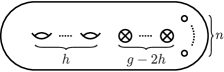
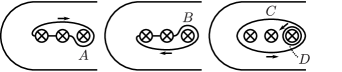
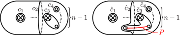
For and , let denote a compact non-orientable surface of genus with boundary components, that is, is a surface obtained by removing open disks from a connected sum of real projective planes. For and , let denote a compact orientable surface of genus with boundary components, that is, is a surface obtained by removing open disks from a connected sum of tori. As shown in Figure 1, we can regard as a surface obtained by attaching Möbius bands to boundary components of , for . We call these attached Möbius bands crosscaps.
The mapping class group of , denoted by , is the group consisting of isotopy classes of all diffeomorphisms of which fix the boundary pointwise. The mapping class group of , denoted by , is the group consisting of isotopy classes of all orientation-preserving diffeomorphisms of which fix the boundary pointwise. It is well known that is generated by only Dehn twists (see [3, 17, 4]). On the other hand, can not be generated by only Dehn twists. As generators of , other than Dehn twists, crosscap slides or crosscap transpositions are needed (see [16, 18]). Let us consider the subgroup of generated by all Dehn twists, denoted by . We call the twist subgroup of .
We now explain about the history of studies on presentations for , and . Finite presentations for were given by Hatcher-Thurston [10] and Harer [9], and subsequently simplified by Wajnryb [28] and Matsumoto [20] for . Gervais [8] and Labruère-Paris [15] gave finite presentations of for . Gervais [7] gave an infinite presentation for by using the presentation for given in [9, 28], and then Luo [19] simplified its presentation. Finite presentations for , , and ware given by [16], [23], [2] and [27] respectively. Note that and are trivial (see [5]). Paris-Szepietowski [22] gave a finite presentation of for with . Stukow [25] gave another finite presentation of for with , applying Tietze transformations for the presentation of given in [22]. The second author [21] gave an infinite presentation of for and , using the presentation of given in [25], and then, following this work, the authors [12] gave an infinite presentation of for and . It is known that is the index subgroup of (see [18]). Stukow [26] gave a finite presentation of for with , applying the Reidemeister-Schreier method for the presentation of given in [25] (see Theorems 2.5 and 2.6).
In this paper, we give an infinite presentation of for and (see Theorem 1.1), mainly using the presentation of given in [26] and Birman exact sequences on mapping class groups of non-orientable surfaces.
Through this paper, the product of mapping classes and means that we apply first and then . Moreover we do not distinguish a loop from its isotopy class.
1.2. Main result
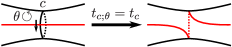
For a simple closed curve of , a regular neighborhood of is either an annulus or a Möbius band. We call a two sided or a one sided simple closed curve respectively. For a two sided simple closed curve , we can take two orientations and of a regular neighborhood of . The right handed Dehn twist about a two sided simple closed curve with respect to is the isotopy class of the map described as shown in Figure 2. does not depend on a choice of a representative curve of the isotopy class of and its regular neighborhood. We remark that although the Dehn twist was defined for an oriented simple closed curve in [21, 12], in this paper we do not consider an orientation of a simple closed curve in the definition of the Dehn twist. We write if the orientation is given explicitly. That is, the direction of the twist is indicated by an arrow written beside as shown in Figure 2.
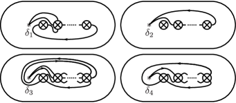
We denote by the orientation of a regular neighborhood of induced from , for a two sided simple closed curve of and . Let , , and be simple closed curves with arrows as shown in Figure 3. admits following relations.
-
(1)
if bounds a disk or a Möbius band.
-
(2)
.
-
(3)
for .
-
(4)
if is odd,
if is even. -
(5)
.
We can check the relations (1) and (2) easily. The relations (3), (4) and (5) are called a conjugation relation, a -chain relation, a lantern relation respectively. These are famous relations on mapping class groups. In the relation (3), if , or , and the orientations and are compatible, then the relation can be rewritten as a commutativity relation or a braid relation respectively.
Our main result is as follows.
Theorem 1.1.
For and , admits a presentation with a generating set
The defining relations are
-
(1)
if bounds a disk or a Möbius band,
-
(2)
,
-
(3)
all the conjugation relations for ,
-
(4)
all the -chain relations,
-
(5)
all the lantern relations,
Remark 1.2.
Remark 1.3.
Here is the outline of this paper. In Section 2, we explain what we need to prove our main result. In Section 3, we prove that the infinitely presented group with the presentation in Theorem 1.1 is isomorphic to with a presentation which is already known, for . In Section 4, we complete the proof of Theorem 1.1, by induction on .
2. Preliminaries
In this section, we explain what we need to prove our main result Theorem 1.1. In Section 2.1, we define the capping map, the point pushing map, the forgetful map and the crosscap pushing map on mapping class groups for non-orientable surfaces. In Section 2.2, we introduce a finite presentation of for and .
2.1. Homomorphisms on mapping class groups of non-orientable surfaces
We first define the capping map, the point pushing map and the forgetful map on mapping class groups of non-orientable surfaces. Take a point in the interior of . Let denote the group consisting of isotopy classes of all diffeomorphisms of which fix and the boundary pointwise. We can regard as a complement of an open disk neighborhood of in . The natural embedding induces the homomorphism
which is called the capping map. The point pushing map
is defined as follows. For any loop , is described by pushing once along . The forgetful homomorphism
is defined naturally, that is, does not necessarily fix .
Next, we consider exact sequences on mapping class groups of non-orientable surfaces. Let denote the subgroup of consisting of elements which preserve a local orientation of , and the subgroup of generated by two sided simple loops. We have the exact sequences
| (1) | |||
| (2) |
The second sequence is called the Birman exact sequence, introduced by Birman [1]. Note that is injective except for the case . For details see [1, 14, 24, 6, 22].
Remark 2.1.
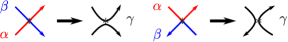
For a simple loop , we take an orientation of a regular neighborhood of . Let and be the right side boundary curve and the left side boundary curve of the regular neighborhood of for the direction of , respectively, where the left and right sides are determined by . Then we have , where and are the orientations compatible with (see Figure 4).
Remark 2.2.
Let , and be simple loops with . If and intersect transversally at only as shown in Figure 5, then the relation is obtained from the relation (3) of Theorem 1.1 (see Lemma 5.4 in [12]). If and intersect tangentially at only as shown in Figure 5, then the relation is obtained from the relation (5) of Theorem 1.1 and a relation , where is a simple closed curve bounding a disk neighborhood of (see Lemma 5.2 in [12]). We call this relation the extended lantern relation.
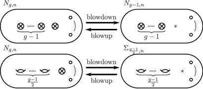
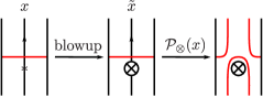
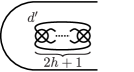
Finally, we define the crosscap pushing map. Let be a surface obtained by shrinking some crosscap of into a point. We call this operation the blowdown with respect to the crosscap. Note that is diffeomorphic to either or (see Figure 6). Let be the shrinked point of . Conversely, we can obtain from , and call this operation the blowup with respect to . The crosscap pushing map
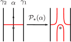
is defined as follows. For , let be an oriented loop of induced from by the blowup with respect to . is described by pushing the crosscap, which is obtained by the blowup with respect to , once along (see Figure 7).
Remark 2.3.
For a two sided simple loop , we take an orientation of a regular neighborhood of . Let and be the right side boundary curve and the left side boundary curve of the regular neighborhood of for the direction of , respectively, where the left and right sides are determined by . We also denote by and loops of induced from and by the blowup with respect to , respectively. Then we have , where and are the orientations of regular neighborhoods of and induced by the blowup with respect to from the orientations of regular neighborhoods of and which are compatible with , respectively.
Remark 2.4.
Let , and be two sided simple loops with . If and intersect transversally at only as shown in Figure 5, then the relation is obtained from the relarions (3) of Theorem 1.1 (see Lemma 5.4 in [12]). If and intersect tangentially at only as shown in Figure 5, then the relation is obtained from the relations (1) and (5) of Theorem 1.1 (see Lemma 5.2 in [12]).
2.2. A finite presentation for
For and we have the short exact sequence
| (3) |
(see [16, 18]). Using the Reidemeister Schreier method for a presentation of , we can obtain a presentation of .
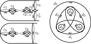
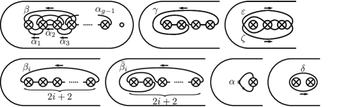
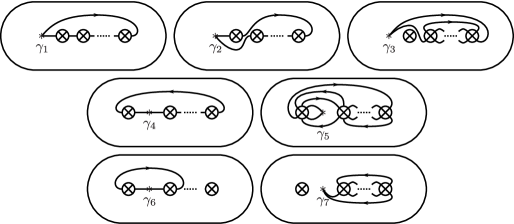
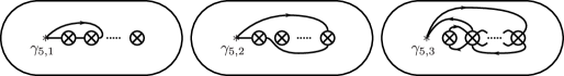
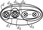
For , let , , , and be simple closed curves of with arrows as shown in Figure 8, and if is even, , , and simple closed curves of with arrows as shown in Figure 8. Let be an oriented simple loop of based at induced from by the blowdown with respect to the first crosscap, as shown in Figure 8. For simplicity, we denote , , , , , , and . Note that , where is a simple close curve of with an arrow as shown in Figure 8. For and , admits a finite presentation given in Theorems 2.5, 2.6 or Lemma 2.7.
Theorem 2.5 (Theorem 3.1 in [26]).
If is odd or , then admits a presentation with generators , , , and , for . The defining relations are
-
(A1)
for , ,
-
(A2)
for ,
-
(A3)
for , ,
-
(A4)
for ,
-
(A5)
for ,
-
(A6)
for ,
-
()
for , ,
-
()
for , ,
-
()
,
-
()
for ,
-
()
,
-
()
for , ,
-
()
for , ,
-
()
for , ,
-
()
for , ,
-
()
for , ,
-
()
for ,
-
()
,
-
()
,
-
()
for ,
-
()
,
-
()
,
-
()
for ,
-
()
for , ,
-
()
for ,
-
()
for ,
-
()
for ,
-
()
for , .
If is even, then admits a presentation with generators , , , , , and additionally , , , . The defining relations are relations -, -, - and additionally
-
(A7)
, ,
-
(A8)
for ,
-
(A9a)
for ,
-
(A9b)
for ,
-
()
, for ,
-
()
for ,
-
()
where , , and ,
-
()
for ,
-
()
for ,
-
()
for ,
-
()
for .
Theorem 2.6 (Theorem 3.2 in [26]).
If is odd, then the group is isomorphic to the quotient of the group with the presentation given in Theorem 2.5 obtained by adding a generator and relations
-
()
,
-
()
,
-
()
for ,
-
()
,
-
()
,
-
()
,
-
()
.
Moreover, relations , , are superfluous.
If is even, then the group is isomorphic to the quotient of the group with the presentation given in Theorem 2.5 obtained by adding a generator and relations
-
()
,
-
()
,
-
()
for ,
-
()
,
-
()
,
-
()
,
-
()
.
Moreover, relations , , are superfluous.
Lemma 2.7.
-
(1)
and are trivial.
-
(2)
.
-
(3)
.
-
(4)
.
Proof.
Note that is generated by the image of , in the sequence (3) at the beginning of Section 2.2.
-
(1)
and are trivial (see Theorem 3.4 in [5]). Thus and are also trivial.
-
(2)
We have the presentation
(see Lemma 5 in [16]). Using the Reidemeister Schreier method for this presentation, we obtain the presentation
-
(3)
We have the presentation
(see Theorem A.7 in [23]). Using the Reidemeister Schreier method for this presentation, we obtain the presentation
-
(4)
We have the presentation
(see Theorem 3 in [2]). Using the Reidemeister Schreier method for this presentation, we obtain the presentation
∎
3. Proof of Theorem 1.1 for and
In this section, we prove Theorem 1.1 for and , using the presentation of given in Theorems 2.5, 2.6 and Lemma 2.7.
Let be the infinitely presented group with the presentation given in Theorem 1.1, and the presentation for given in Theorems 2.5, 2.6 or Lemma 2.7. Denote by the free group freely generated by . Let be the natural projection and the homomorphism defined as for any . We consider a correspondence
satisfying . Showing the following proposition, we will obtain Theorem 1.1 for and .
Proposition 3.1.
For and , is an isomorphism.
Let be the homomorphism defined as for any . Since in clearly, is well-defined. By the definitions of and , it is clear that is the identity map if is a homomorphism. Hence in order to prove Proposition 3.1, what we need is to show well-definedness and surjectivity of . In Sections 3.1 and 3.2, we see well-definedness and surjectivity of respectively.
3.1. Well-definedness of
In order to see well-definedness of , it suffices to show that in for any . More precisely, we check that any relation and relator of in Theorems 2.5, 2.6 and Lemma 2.7 are obtained from the relations (1)-(5) of in Theorem 1.1 and the relation assigned in Remark 1.3.
First we notice that the relations , and hold since each of the pairs , , for , and for , coincides as mapping classes from the definition of loops in Figure 8. We may also treat the relation as a definition of . It is easy to check that any relator of in Lemma 2.7 is obtained from the relations (1)-(4) in Theorem 1.1. In particular, for the relator of , recall Remark 1.2. The relations , , , , , , , , , , , , , , , , , , , , , , , , , , and are obtained by repeating the relation (3) in Theorem 1.1. The relations , , , , , and come from relations of mapping class groups of orientable surfaces (see Theorem 1.3 in [20]), and hence these relations are obtained from the relations (3), (4) and (5) in Theorem 1.1 by Theorem in [19]. The relations and are obtained from the relations (1) in Theorem 1.1 and assigned in Remark 1.3. Thus it suffices to show that the relations , , , , , , , , , and are satisfied in .
Recall the simple closed curves and the simple loop as shown in Figure 8.
3.1.1. On the relation
The relation can be rewritten as follows.
Similarly, the relation can be rewritten as follows.
Let , , , and be simple closed curves with arrows as shown in Figure 9. Repeating the relation (3), we have , and . Assuming that holds in , we calculate
Note that bounds . Thus the relation is satisfied in , by Section 3.1.2.

3.1.2. On the relations and
Let , , and be simple closed curves with arrows as shown in Figure 10. Repeating the relation (3), we have and . In addition, by the relations (1) and we have . Hence we calculate
Note that bounds . Thus the relation is satisfied in .
3.1.3. On the relations and
Let , , , and be simple closed curves with arrows as shown in Figure 11. Repeating the relation (3), we have and . Then we calculate
and hence . Note that and bound . Thus the relation is satisfied in .

In addition, repeating the relation (3), we have , and . Then we calculate
and hence . Note that bounds . Thus, since , the relation is satisfied in .
3.1.4. On the relations and
Let , , and be simple closed curves with arrows as shown in Figure 12. Repeating the relation (3), we have , and . By the relation (5) we see
and by the relations (1) and (3) we see
Note that bounds . Thus the relation is satisfied in .

3.1.5. On the relation
We calculate
Let . Similarly, we calculate
We show that . Since a regular neighborhood of is diffeomorphic to , by the relations (1) and , we have . We calculate
It suffices to show the equality
Let , and be oriented simple loops based at which is a point obtained by the blowdown with respect to the first crosscap in when is odd, as shown in Figure 13 (a), and and simple closed curves with arrows as shown in Figure 13 (b). By the relations (1), and Remark 2.3, we have , , and . Hence by Remark 2.4, we calculate
On the other hand, we see
In addition, by the calculation similar to the beginning of Section 3.1.5, we see
and hence
Let , , and be oriented simple loops based at which is a point obtained by the blowdown with respect to the second crosscap, as shown in Figure 13 (a), , and oriented simple loops based at which is a point obtained by the blowdown with respect to the first crosscap, as shown in Figure 13 (b), and a simple closed curve with an arrow as shown in Figure 13 (c). By the relations (3), and Remark 2.3, we have ,
, and . Hence by Remark 2.4, we calculate
Thus the relation is satisfied in .

3.1.6. On the relation
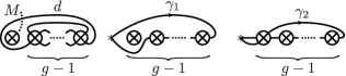
For , let be an oriented simple loop based at which is a point obtained by the blowdown with respect to the first crosscap, as shown in Figure 14, and .
We now prove the following lemma.
Lemma 3.2.
In , we have for .
Proof.
3.1.7. On the relation
In , is defined as and we have the relation (see Theorem 2.2 in [26]). In addition, note that Lemma 3.2 holds even if is even. Hence we calculate
where is defined in Section 3.1.6. Let and be oriented simple loops based at which is a point obtained by the blowdown with respect to the first crosscap, as shown in Figure 15 (a). Repeating the relation (3), we have . In addition, by Remark 2.4, we have . Let and be oriented simple loops based at which is a point obtained by the blowdown with respect to the first crosscap, as shown in Figure 15 (a). Repeating the relation (3), we have . In addition, by Remark 2.4, we have . Let and be simple closed curves with arrows as shown in Figure 15 (b). By the relation and Remark 2.3, we have and . Hence we calculate
Thus the relation is satisfied in .

3.1.8. On the relation
Note that the relation is obtained from the relations and . We call this relation . By the equality which appeared in Section 3.1.7, we calculate
Thus the relation is satisfied in .
Therefore well-definedness of follows.
3.2. Surjectivity of
For any simple closed curve of , we denote the complement of the interior of a regular neighborhood of by . If and are diffeomorphic, there exists with for . In particular, if and are two sided, we have for some orientation and .
For any two sided simple closed curve of where , is diffeomorphic to either one of
-
•
, where ,
-
•
, where is even,
-
•
, where ,
-
•
, where and ,
-
•
, where and is even.
For each case, we would like to find a word on such that , where is defined at the beginning of Section 3.
3.2.1. The case where is diffeomorphic to or
3.2.2. The case where is diffeomorphic to
When , since by the relation (1), we obtain . When , there exists such that , where is the boundary curve of a regular neighborhood of which is diffeomorphic to , as shown in Figure 16. Note that we have for some , by the relation . If , there exists a word on . Then we obtain , repeating the relations (3) and . If , there exists a word on . Since , and for , we obtain , repeating the relations (3) and .
3.2.3. The case where is diffeomorphic to
When , since by the relation (1), we obtain . When , there exists such that , where appeared in Figure 8. If , there exists a word on . Then we obtain , repeating the relation (3). If , there exists a word on . Since , we have , repeating the relation (3). When , we take simple closed curves as shown in Figure 17. By induction on , we can suppose that is described as a word on for . Hence we obtain for some , by the relations (2) and (5).
3.2.4. The case where is diffeomorphic to
When , since by the relation (1), we obtain . When , is described as shown in Figure 18, for some model of . Let and be oriented loops of based at as shown in Figure 18, where is the point obtained by the blowdown with respect to the crosscap in Figure 18. Note that and are two sided since is even when . In addition, when , is diffeomorphic to for and , where and appeared in Figure 8. Hence by Remark 2.3, we can describe for some , for and . If , is represented by a word on , and hence is a word on . If , is represented by a word on . Since , is a word on . We denote the word presentation of on by . Then we calculate , by Remarks 2.3 and 2.4. When , we take simple closed curves as shown in Figure 17, similar to Section 3.2.3. Since is diffeomorphic to either , , or , by Section 3.2.3, is described as a word on for . Hence we obtain for some , by the relations (2) and (5).
Therefore surjectivity of follows, and hence the proof of Proposition 3.1 is completed.
4. Proof of Theorem 1.1 for and
Recall the capping map , the point pushing map and the forgetful map defined in Section 2.1. Let , then for and , from the sequences (1) and (2) in Section 2.1, we have the short exact sequences
| (4) | |||
| (5) |
Using these sequences and the presentation of given in Section 3, we give the presentation of for and , by induction on .
Note that, in general, as basics on combinatorial group theory, from presented groups and with a short exact sequence , we can give a presentation for as follows. Let be any lift of with respect to , and a word obtained from by replacing each to . For , denote by a word on corresponding to . For , denote by a word on obtained from by replacing to . Let and . Then we have a presentation . For details, for instance see Proposition 1 in 10.2 in [11].
We now show the following proposition, using the sequence (5). Remember the infinite presentation for the group presented in Theorem 1.1.
Proposition 4.1.
For and , suppose , then admits a presentation with a generating set
The defining relations are
-
if bounds a disk or a Möbius band,
-
,
-
all the conjugation relations for ,
-
all the -chain relations,
-
all the lantern relations,
-
all the extended lantern relations defined in Remark 2.2.
Proof.
is a finite rank free group for . However, we consider an infinite presentation for . Let be the group generated by symbols for a non-trivial simple loop , and with the defining relations
-
•
,
-
•
if ,
-
•
if .
Then we have that is isomorphic to (see Theorem 1.2 in [13]). So gives an infinite presentation for . By this we identify with .
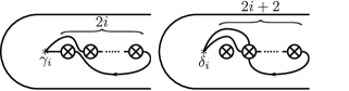
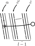
We take a simple path of between and the -st boundary component. For a simple closed curve of , let be a simple closed curve of corresponding to which does not intersect , as shown in Figure 19.
By the sequence (5), is generated by
-
•
for any simple closed curve of and
-
•
for any generator of .
The defining relations are
-
•
for the lift of any with respect to ,
-
•
-
–
,
-
–
for any , and satisfying ,
-
–
for any , and satisfying and
-
–
-
•
for any and ,
where is a word corresponding to on . We denote this presentation by . In addition, let be the infinitely presented group with the presentation given in Proposition 4.1. We show that is isomorphic to .
Denote by the free group freely generated by . Let be the natural projection and the homomorphism defined as for any . Note that, by Remark 2.1, is also in for any generator of . Hence is well-defined. We consider a correspondence
satisfying . We show that is an isomorphism.
First we show well-definedness of . In the first relation of , from the definition of , it is clear that for any . Hence the first relation of is either one of the relations -. In the second relation of , the relation is trivial. The relation is obtained from the relations or by Remark 2.2. The relation is the relation . In the third relation of , we have , and hence it is the relation . Therefore, any relation of is satisfied in . So is well-defined as a homomorphism.
Next we show bijectivity of . Let be the homomorphism defined as for any . Since in clearly, is well-defined. By the definitions of and , it is clear that is the identity map, and hence is injective. For any , if intersects transversally at points, there exist and such that , as shown in Figure 20, by Remark 2.3. We notice that intersects transversally at points. By induction on the intersection number of and , we see that is a product of some and some ’s. Hence is surjective, and so bijective.
Therefore is the isomorphism. Thus the claim is obtained. ∎
Finally we complete the proof of Theorem 1.1.
Proof of Theorem 1.1.
From the case where of Theorem 1.1, Proposition 4.1 and the sequence (4), by induction on , is generated by
-
•
the natural lift of with respect to and
-
•
the Dehn twist about the -th boundary curve ,
that is, generate . In addition has the relations
-
•
for the lift of any relator of with respect to and
-
•
,
where for some integer corresponding to . In the first relation, it is clear that if is a relator corresponding to the relations - of Proposition 4.1. On the other hand, if is a relator corresponding to the relation of Proposition 4.1, then for some . Hence the first relation is either one of the relation (1)-(5). In the second relation, it is clear that , and hence it is the relation (3).
Thus we complete the proof. ∎
Acknowledgement
The authors would like to express their gratitude to Susumu Hirose for his useful comments.
References
- [1] J. S. Birman, Mapping class groups and their relationship to braid groups, Comm. Pure Appl. Math. 22 (1969), 213–238.
- [2] J. S. Birman and D. R. J. Chillingworth, On the homeotopy group of a non-orientable surface, Proc. Cambridge Philos. Soc. 71 (1972), 437–448. Erratum: Math. Proc. Cambridge Philos. Soc. 136 (2004), no. 2, 441.
- [3] M. Dehn, Die Gruppe der Abbildungsklassen, Das arithmetische Feld auf Flächen, Acta Math. 69 (1938), no. 1, 135–206.
- [4] M. Dehn, Papers on group theory and topology, Springer-Verlag, New Tork, 1987.
- [5] D. B. A. Epstein, Curves on -manifolds and isotopies, Acta Math. 115 (1966), 83–107.
- [6] B. Farb and D. Margalit, A primer on mapping class groups, Princeton Mathematical Series, 49.
- [7] S. Gervais, Presentation and central extensions of mapping class groups, Trans. Amer. Math. Soc. 348 (1996), no. 8, 3097–3132.
- [8] S. Gervais, A finite presentation of the mapping class group of a punctured surface, Topology 40 (2001), no. 4, 703–725.
- [9] J. Harer, The second homology group of the mapping class group of an orientable surface, Invent. Math. 72 (1983), no. 2, 221–239.
- [10] A. Hatcher and W. Thurston, A presentation for the mapping class group of a closed orientable surface, Topology 19 (1980), no. 3, 221–237.
- [11] D. L. Johnson, Presentations of groups, Second edition. London Mathematical Society Student Texts, 15. Cambridge University Press, Cambridge, 1997.
- [12] R. Kobayashi and G. Omori, An infinite presentation for the mapping class group of a non-orientable surface with boundary, Osaka J. Math., 59 (2) (2022), 269–314.
- [13] R. Kobayashi, Infinite presentations for fundamental groups of surfaces, Hiroshima Math. J., to appear.
- [14] M. Korkmaz, Mapping class groups of nonorientable surfaces, Geom. Dedicata 89 (2002), 109–133.
- [15] C. Labruère and L. Paris, Presentations for the punctured mapping class groups in terms of Artin groups, Algebr. Geom. Topol. 1 (2001), 73–114.
- [16] W. B. R. Lickorish, Homeomorphisms of non-orientable two-manifolds, Proc. Cambridge Philos. Soc. 59 (1963), 307–317.
- [17] W. B. R. Lickorish, A finite set of generators for the homeotopy group of a -manifold, Proc. Cambridge Philos. Soc. 60 (1964), 769–778.
- [18] W. B. R. Lickorish, On the homeomorphisms of a non-orientable surface, Proc. Cambridge Philos. Soc. 61 (1965), 61–64.
- [19] F. Luo, A presentation of the mapping class groups, Math. Res. Lett. 4 (1997), no. 5, 735–739.
- [20] M. Matsumoto, A presentation of mapping class groups in terms of Artin groups and geometric monodromy of singularities, Math. Ann. 316 (2000), no. 3, 401–418.
- [21] G. Omori, An infinite presentation for the mapping class group nonorientable surface, Algebr. Geom. Topol. 17 (2017), no. 1, 419–437.
- [22] L. Paris and B. Szepietowski, A presentation for the mapping class group of a nonorientable surface, Bull. Soc. Math. France 143 (2015), no. 3, 503–566.
- [23] M. Stukow, Dehn twists on nonorientable surfaces, Fund. Math. 189 (2006), no. 2, 117–147.
- [24] M. Stukow, Commensurability of geometric subgroups of mapping class groups, Geom. Dedicata 143 (2009), 117–142.
- [25] M. Stukow, A finite presentation for the mapping class group of a nonorientable surface with Dehn twists and one crosscap slide as generators, J. Pure Appl. Algebra 218 (2014), no. 12, 2226–2239.
- [26] M. Stukow, A finite presentation for the twist subgroup of the mapping class group of a nonorientable surface, Bull. Korean Math. Soc. 53 (2016), no. 2, 601–614.
- [27] B. Szepietowski, A presentation for the mapping class group of the closed non-orientable surface of genus 4, J. Pure Appl. Algebra 213 (2009), no. 11, 2001–2016.
- [28] B. Wajnryb, A simple presentation for the mapping class group of an orientable surface, Israel J. Math. 45 (1983), no. 2-3, 157–174.