An -Adaptive Sampling Algorithm for Dispersion Relation Reconstruction of 3D Photonic Crystals
Abstract
In this work we investigate the computation of dispersion relation (i.e., band functions) for three-dimensional photonic crystals, formulated as a parameterized Maxwell eigenvalue problem, using a novel -adaptive sampling algorithm. We develop an adaptive sampling algorithm in the parameter domain such that local elements with singular points are refined at each iteration, construct a conforming element-wise polynomial space on the adaptive mesh such that the distribution of the local polynomial spaces reflects the regularity of the band functions, and define an element-wise Lagrange interpolation operator to approximate the band functions. We rigorously prove the convergence of the algorithm. To illustrate the significant potential of the algorithm, we present two numerical tests with band gap optimization.
Key words: -adaptive sampling algorithm, photonic crystals, band gap maximization, parameterized Maxwell eigenvalue problem
1 Introduction
Photonic crystals (PhCs) are periodic nanostructures typically made from dielectric materials and are widely used in optics for wave manipulation and control [26]. For some specially designed PhCs structures, electromagnetic waves with frequencies in certain ranges cannot propagate in the crystals; these prohibited ranges are so-called band gaps and the knowledge of their position or the ability to design for specific ranges underpin many important applications, including optical transistors, photonic fibers and low-loss optical mirrors [54, 43, 49, 29]. The dispersion relation describes the dependence of wave frequency on its wave vector when the wave passes through certain materials. Photonic band gaps offer numerous benefits in practical applications, e.g., waveguides, cavities, and photonic crystal fibers [12, 8, 52, 32]. Notably there is a parallel field in acoustics and mechanical vibration, phononic crystals [30], where band gaps and periodic media are used to filter and control elastic waves and design devices. In binary systems (i.e., PhCs composed of two materials), the appearance, size, and location of band gaps rely on various factors, including filling fraction, lattice symmetry, topology of constituent material phases, and the contrast between the permittivity of materials [26]. By effectively controlling these parameters, it is possible to design periodic composite materials that possess desired photonic band gaps, thereby achieving excellent performance in practical applications.
The behavior of electromagnetic waves is described mathematically by Maxwell’s equations [25] and the band gaps correspond to the gaps in the spectrum of the Maxwell operator with periodic coefficients. Thus, the task of dispersion relation reconstruction or the numerical simulation of electromagnetic waves inside PhCs can be transformed into the approximation of the Maxwell eigenvalue problem. For infinite crystals with perfect periodicity, Bloch’s theorem reduces the task to a set of parameterized Maxwell eigenvalue problems defined in the unit cell with periodic boundary conditions. The associated parameter is the so-called wave vector , which varies in the irreducible Brillouin zone (IBZ) [28]. The th band function , which is the square root of the th largest eigenvalue up to a constant, is regarded as a function of the wave vector for all and the band gap represents the separation between two adjacent band functions. Thus, computing the th band function boils down to solving an infinite number of Maxwell eigenvalue problems. To create these band gaps, it is imperative that the permittivity exhibits distinct values in both the inclusion and the background of the unit cell, and that the magnitude difference, referred to as the “contrast”, is often substantial. However, solving the Maxwell eigenvalue problems with high-contrast and piecewise constant coefficients presents notorious numerical challenges due to, e.g., spurious modes [48], and an indefinite large-scale linear system.
To reduce the computational burden, a natural approach is to reduce the number of parameters by constraining to a coarse mesh within the IBZ or its boundaries. Nonetheless, recent research has uncovered instances where tiny band gaps, e.g., the so-called avoided crossings, observed within this simplified approximation, vanish upon the inclusion of additional -points or the enhancement of eigenvalue precision [23, 40, 13]. This drawback greatly affects some application areas of photonic materials in which the requirements are very sensitive to tiny band gaps. For example, it is important to avoid the smallest band gaps in the manufacture of Large-Pitch PhC fiber for a larger output average power [19] while the leakage channel fibers exploit the smallest band gaps [18]. There is a conflict between desiring high accuracy (i.e., sampling at many over the IBZ), and the computational cost in doing so for three-dimensional (3D) structures. Thus, it is of huge importance to develop algorithms that use as few sampling points for PhCs band function calculations as possible and yet accurately characterize the band functions.
In this work, we extend the -adaptive sampling method [50] (for 2D PhCs, described by parameterized Helmholtz eigenvalue problem) to the 3D cases, by interpolating the band functions elementwise on an adaptive mesh, and demonstrate its efficiency on the band gap maximization problem [10, 53, 22]. First, we adaptively refine the mesh in the parameter domain, cf., Algorithm 1, by element-wise indicator (3.1) and tolerance (3.2), which adaptively refines elements containing singularities, cf. Theorem 3.1. Second, we construct a conforming finite element space (3.5) on the adaptive mesh, and derive element-wise interpolation by identifying a set of basis functions for the local polynomial space. Third, we establish the -adaptive sampling algorithm in Algorithm 2, and rigorously justify its convergence in Theorems 4.5 and 4.6. The resulting method allows approximating band functions accurately using significantly fewer sampling points, thus making the band gap maximization more efficient.
To demonstrate the efficiency of the algorithm, we employ two models of 3D PhCs, which consist of layered cubic structures with silicon blocks and spheres embedded in air. By optimizing the dimensions of these blocks and the radius of the spheres, we identify an optimal unit cell structure that maximizes the band gap. These experiments show the challenges of calculating the band function of 3D PhCs and showcase the process of the adaptive interpolation algorithm. To verify the performance of Algorithm 2, we display its convergence history and compare it with the uniform refinement.
The rest of this paper is organized as follows. In Section 2, we summarize the derivation of band functions for 3D PhCs and discuss the properties of band functions. We also outline the challenges associated with computing the Maxwell eigenvalue problem and describe the -conforming -modified Nédélec edge finite element method (FEM). In Section 3, we extend the -adaptive sampling method [50] to 3D cases, and in Section 4, we present a convergence analysis of this method. In Section 5, we define the shape optimization problem, which aims to find the maximal band gap in cubic lattices with silicon blocks and spheres. We also include numerical experiments in this section to verify our results. Finally, in Section 6, we provide a conclusion and potential future works.
2 Problem formulation
We recap in this section the derivation of the band function computation for 3D PhCs as a parametrized Maxwell eigenvalue problem (2.5) and its weak formulation (2.7). Then we describe its finite element discretization by the - conforming -modified Nédélec edge element method (2.9). Finally, we provide an efficient approximation of the gradient of the band functions.
2.1 Maxwell equations, eigenvalue problem, and the weak formulation
In SI convention, the time harmonic Maxwell equations with and for linear, non-dispersive, and nonmagnetic media, with free charges and free currents, consist of a system of four equations [25]
| (2.1a) | ||||
| (2.1b) | ||||
| (2.1c) | ||||
| (2.1d) | ||||
where is the electric field, is the magnetic field, the scalar is the frequency of the electromagnetic wave, is the vacuum permeability, is the vacuum permittivity, and is the relative permittivity.
Applying the curl operator to (2.1b) and using (2.1a) give the equations for the magnetic field
| (2.2) |
with , where is the speed of light. The electric field can be derived from (2.1b):
| (2.3) |
which implies (2.1c). The above two equations form the governing system of 3D PhCs.
Next, 3D periodic PhCs possess a discrete translational symmetry in [26], i.e., the relative permittivity satisfies
The primitive lattice vectors, denoted as , are the shortest possible vectors that satisfy this condition which span the unit cell . For example, square lattice has primitive lattice vectors for , with being the lattice constant and being the canonical basis in . Additionally, the reciprocal lattice vectors, , are defined by the property
| (2.4) |
which generate the so-called reciprocal lattice. The elementary cell of the reciprocal lattice is the (first) Brillouin zone , i.e., the region closer to a certain lattice point than to any other lattice points in the reciprocal lattice. Note that if the materials in the unit cell have additional symmetry, e.g. mirror symmetry, we can further restrict to the irreducible Brillouin zone (IBZ).
Based on Bloch’s theorem [28], the spectrum corresponding to a periodic structure in the full space is equivalent to the union of all spectra corresponding to the quasi-periodic problems in the unit cell. Thus, we apply Bloch’s theorem and aim to find the wave function taking the form of a plane wave modulated by a periodic function. Mathematically, it can be written as , where is a periodic function satisfying for and is the wave vector varying in the Brillouin zone . Thus, by Bloch’s theorem, the eigenvalue problem (2.2) reduces to
| (2.5) |
where , varies in the Brillouin zone , and satisfies the periodic boundary conditions with being the primitive lattice vector for . For all , we can enumerate these eigenvalues in a non-decreasing manner (with their multiplicities counted) as
Then is an infinite sequence with being a continuous function with respect to the wave vector and when [21].
Below we state the regularity of band functions, which can be proved in a similar manner as the 2D case [51]. Here, is the space of Lipschitz continuous functions in the Brillouin zone and denotes the space of piecewise analytic functions with a zero Lebesgue measure of singular point set composed of points of degeneracy (i.e., the set of points at which certain band functions intersect, with zero Lebesgue measure). Throughout, the set of singular points is denoted by .
Theorem 2.1 (Piecewise analyticity and Lipschitz continuity of band functions).
For 3D periodic PhCs, for all .
Next, we introduce the weak formulation to (2.5). We first introduce useful notation for function spaces. For an open, bounded and simply-connected Lipschitz domain , we define the space of square integrable functions equipped with the inner product and the corresponding norm by , where denotes the complex conjugate. We denote by the usual Sobolev space with norm
We also write , and , for the inner products and norms of vector-valued functions spaces , , respectively. Let be the standard inner product on the Sobolev space and be the inner product on . Also we will use the following spaces for the weak formulation:
Here is the unit outward normal vector to . The periodic Sobolev spaces , , are the closures of the spaces , , with respect to the Sobolev space norms ,, induced by the inner product mentioned above respectively. The periodic space is the closure of the space with respect to the norm .
Then the spaces for the weak formulation are given by
| (2.6) |
For and , we define the sesquilinear forms
Then the variational formulation to (2.5) can be written in a mixed form: for a given , find non-trivial eigentriplets such that
| (2.7) |
Finally, we introduce a regularity assumption for the finite element analysis [4, Assumption ],
Assumption 2.1.
There exists such that is continuously embedded in . Moreover, for a given and for any , let satisfy
Then there is and , such that and .
2.2 - conforming -modified Nédélec edge FEM
In this section we describe the discretization of problem (2.7) for each wave vector using the - conforming -modified Nédélec edge element method, which is stable with respect to . Since the divergence of the curl of any vector is zero, taking the divergence on both sides of the first equation in (2.5) gives its second equation. Furthermore, the zero eigenvalue of (2.5) has an infinite multiplicity since the curl operator has an infinite-dimensional kernel. Thus, a discretization of the eigenvalue problem (2.5) solely using the scalar node-based FEM may contain non-physical solutions (i.e., spurious modes [48]). Indeed, most eigenvalue solvers are inefficient when dealing with such eigenvalue problems [2].
To eliminate these spurious modes, the standard approach is to use the edge FEM and add the constraint (2.5) explicitly [31, 48]. The Lagrange multiplier in the mixed form in (2.7) is one common approach to add the divergence constraint to the system. Also, several methods have been proposed to eliminate this large null space [14, 11, 24, 38, 36, 35], including the special -conforming -modified Nédélec edge elements [15, 4] and the mixed discontinuous Galerkin (DG) formulation with modified Nédélec basis functions [35]. The - conforming -modified Nédélec edge element method was first proposed and analyzed in [14, 15] under strong regularity restrictions and in the case of uniform mesh sequences, with an improved analysis under minimal assumptions on the regularity of the eigensolutions and on the mesh sequences [4]. We recap the Nédélec edge element method below.
Let be a periodic, shape-regular, conformal tetrahedral mesh for aligned with the possible discontinuities of , where the phrase “periodic” means that the meshes are the same on each pair of the boundary. Let , where is the diameter of . We denote the set of all edges by and the set of all vertexes by . The conforming finite element spaces of (2.6) are [4]
| (2.8) | ||||
where is the space of local polynomials of total degree less than or equal to on , and is the space of vector polynomials with the form with .
2.3 Gradient of in the parameter domain
Next, we derive the formula of the gradient for and , and provide its numerical approximation. Recall that denotes the canonical basis in .
Theorem 2.3.
Let the non-trivial eigentriplet be the solution to the weak formulation (2.7) for any . Then there holds
| (2.11) |
Proof.
We abbreviate and to and . By definition, for all , there holds
Upon utilizing the formula for ,
and taking the partial derivative of (2.7) with respect to , we obtain
with , where and are defined as
By repeating the argument for [51, Theorem 3.6], we can derive the derivatives of the eigenvalue with respect to through , and arrive at
| (2.12) |
since the eigenfunction is normalized, i.e., . Following equation (2.12), we find
This completes the proof. ∎
The use of modified basis functions (2.8) greatly simplifies the computation of , and hence reduce the computational complexity. For example, for the lowest order Nédélec FEM space with in (2.8), the degrees of freedom for are
Here, denotes the midpoint of edge , identified with the ordered vertices , and represents the unit tangent vector of . Hence, of the lowest order can be expressed as
with and . Similarly, of the lowest-order can be represented by
with and , which has the vertex-based degrees of freedom defined as , for all , is the coordinate of a vertex in .
With the basis functions defined above, we obtain
Together with (2.11), we obtain
Thus, the use of the modified basis functions separates the integral with the parameter , transforming it into a standalone exponential function during the computation. This separation streamlines evaluating the integrals, making it a conventional integration involving parameter-free polynomials.
3 -adaptive sampling method in the parameter domain
In this section, we generalize the -adaptive sampling method [50] from 2D PhCs to 3D PhCs for the purpose of computing the th and th band functions with . We introduce in Section 3.1 an adaptive mesh in the parameter domain which refines the elements containing singularity points, and propose in Section 3.2 an element-wise interpolation operator to reconstruct the target band functions.
3.1 Adaptive mesh generation
We first recall the definition of a regular mesh without hanging nodes [45]. Let be a polygon with straight sides and a mesh be a partition of into open, disjoint tetrahedrons with . For each , we denote by its diameter and the diameter of its largest inscribed ball.
Definition 3.1.
A mesh is said to be a regular mesh without hanging nodes if it satisfies the following conditions. (i) For , is either empty or it consists of a vertex or an entire edge or an entire face of and (ii) there exists a constant such that .
Now we develop a strategy to generate a family of nested regular tetrahedral meshes , , such that is a refinement of . To this end, we introduce several notations for the given regular tetrahedral mesh . The mesh size of is defined as . The collection of all the faces, edges, and vertices over is denoted as , and , respectively. For any , we define its faces as , and the th face is denoted by for . Similarly, we define its edges and vertices as and , and the th edge and vertex are denoted by for , and for . For any , we define the collection of elements having as a face as and the collection of elements having as an edge as . Finally, we define as the space of polynomial functions with total degrees at most on element , and , as the space of polynomial functions of degrees at most on each face and each edge , respectively.
Theorem 2.1 implies that each is a piecewise analytic function of the wave vector , with singular points at the branch points. Our mesh design strategy aims to identify elements within where and are not smooth. To accomplish this, we introduce an element-wise indicator
| (3.1) |
which uses the adjacent values on the vertices of each tetrahedron element to ascertain the regularity of the eigenvalues as functions of within each element. Furthermore, the element-wise tolerance is
| (3.2) |
where is a constant and
is an upper bound of the gradients of with .
Remark 3.1.
In the numerical experiments, we take , which represents a more relaxed tolerance. It reduces the computational cost, while ensuring the expected convergence rate and controlling the maximum error within .
Give a mesh , the collection of marked elements is given by
| (3.3) |
Then we apply the iterated longest edge bisection algorithm (LEB) [42] to divide each marked element into two children elements, which typically follows two steps. First, creating a new vertex at the midpoint of its longest edge and then dividing this tetrahedron by the plane that passes through this new vertex and the two vertices opposite the longest edge. Second, performing additional bisection to avoid any hanging nodes by means of recursive algorithm, which was proven to be finite [42].
We summarize the proposed mesh refinement procedure in Algorithm 1, where the parameters and denote the smallest allowed element size and the maximum number of iterations, respectively.
Next, we show that all elements containing singular points are marked for refinement. For the mesh at the th iteration, let
be a partition of the mesh based upon the singular point set .
Theorem 3.1 ().
Proof.
The proof follows directly from that of [50, Theorem 3.2]. ∎
In practice, we use a practical tolerance given by
| (3.4) |
as a substitute for which only requires for and over , which can be obtained from (2.11).
3.2 Element-wise interpolation over the adaptive mesh
Let be a sequence of nested regular tetrahedral meshes generated by Algorithm 1. First, we establish a finite element space of continuous element-wise polynomial functions as the ansatz space to approximate the target band functions. Then, we define element-wise interpolation operator to reconstruct the target band functions on conforming finite element spaces. First, we introduce the concept of a layer of each element .
Definition 3.2.
The layer of an element is , where is the number of refinements that have been performed on the element in Algorithm 1.
Next, we define the total degree for each element, face and edge.
Definition 3.3 (Element-wise, face-wise and edge-wise spaces of polynomial functions).
For each element , we take as the local interpolation space, with
Here, denotes the ceiling function, the slope parameter will be determined by (4.11) and is the collection of marked elements (3.3). Similarly, for each face , let be the local interpolation space over with , and let be the local interpolation space over for with .
This construction implies
Finally, we define the conforming element-wise polynomial space. On a given mesh with , , and being the element-wise, face-wise, and edge-wise degrees, the global approximation space is given by
| (3.5) |
which is a linear space consisting of continuous piecewise polynomial functions on with predetermined degrees given by the triple .
Now, we introduce the local approximation space on the reference triangular pyramid :
The vertices of are , , and . Let be the face opposite to and let with be the edge with endpoints and . For any with and for , , , (3.5) implies that the local space of polynomial functions over is
| (3.6) |
Note that and if or for certain with . Note also that the dimension of is and the dimension of is
Next we construct a set of basis functions for the local polynomial space . We first partition the degrees of freedom into edge, face, and internal ones according to whether they vanish over the edge, face, and boundary. The basis functions can further be classified into four types: nodal, edge, face, and internal ones, following the standard practice in the community of -adaptive FEMs [1]. It enables defining conforming finite element spaces with nonuniform degrees of polynomials over the mesh.
First, the nodal shape functions are defined as the following four polynomials:
| (3.7) |
Note that for , we have and for .
Second, the set of edge shape functions over each edge for , are
| (3.8) |
where is a polynomial of degree . The edge functions vanish on all vertices and all faces that do not include the edge.
Third, the face shape functions over each face for are defined as
| (3.9) |
Here with denotes the face bubble function and is the space of polynomials defined on with total degree no greater than . Moreover, we set . Clearly, .
Altogether, the set of external shape functions is given by
Let be the basic bubble function on the reference element that vanishes over . Then the set of internal shape functions are defined as
| (3.10) |
Next, we introduce a set of Lagrangian interpolation points over the reference triangular pyramid with the local polynomial space (3.6) such that its restriction to each face and each edge serves as the Lagrangian interpolation points within the face or edge called the Lobatto tetrahedral (LTT) set [37]. First we introduce a 1D grid in the interval comprising a set of sampling points , for , where are the zeros of the th degree Lobatto polynomial. The endpoints are and .
Definition 3.4 (Sampling points over each edge, face and internal).
Suppose the edge degrees on , face degrees on and total degree are , and for , . Then the sampling points are defined below.
-
•
The set of sampling points on all edges are
(3.11) with being the linear transformation maps to .
-
•
The sampling points on are , , , with
(3.12) for , and satisfying , for , and , , , , for . Here, is the face-wise degree on the given face .
-
•
The internal sampling points are introduced at the positions with
(3.13) for , , , and .
Next, we give an interpolation operator , such that for all , there holds
| (3.14) |
First, we introduce the external interpolation . For any function , the external interpolation is a linear interpolation on a set of sampling points on given by Definition 3.4 in the set of external shape functions . Next, we extend from to and denote it as . Then we define the internal interpolation operator as the Lagrange interpolation on internal sampling point set (3.13) using the set of internal shape functions (3.10). Denote the Lebesgue constant of as , i.e.,
| (3.15) |
It has been shown numerically [37, 7] that has moderate growth with respect to the total degree . Finally, we can define the element-wise interpolation by
| (3.16) |
By construction, fulfills the desired properties (3.14). Moreover, the following properties hold. (i) , for all ; (ii) is the Lagrange interpolation on the sampling point set (3.11) along each edge for with ; (iii) is the Lagrange interpolation on the sampling point set (3.12) along each face for ; (iv) is the Lagrange interpolation of on the sampling point set inside (3.13).
For a given mesh , we define the global approximation operator by applying to each element as
| (3.17) |
where the affine transformation ( is invertible and ) maps the reference tetrahedron to the ”physical” element .
Now we can give the following algorithm for approximating and . By sequentially generating the adaptive mesh and the polynomial degree required for each element, each face, and each edge, we can then use the interpolation formula (3.17) to adaptively interpolate for .
4 Convergence analysis
This section is devoted to the convergence analysis of Algorithm 2. We prove an exponential convergence rate in Theorem 4.5 when the number of crossings among is finite, and an algebraic convergence in Theorem 4.6 otherwise. To this end, we first establish the approximation property of the local polynomial interpolation operator in Theorem 4.3. Then we formulate the element-wise approximation property of in Theorems 4.5 and 4.6 under assumption (4.11) on the slope parameter such that the approximation error in the marked element patch dominates.
4.1 Local approximation error
First we establish the approximation property of the local interpolation operator . Recall that for any element-wise, face-wise, and edge-wise degrees , , and , the local space is defined by (3.6). Below the notation stands for that is bounded above by a constant independent of the total degree, face degree, and edge degree.
First, we establish the stability of the external interpolation . Although there is no proof, numerical results show that the Lebesgue constant of the set of sampling points on each face (3.12) is [3]. Hence we make the following assumption
| (4.1) |
Theorem 4.1.
Let (4.1) hold. Then the Lagrange interpolation along each face is stable, for . Moreover, there holds
| (4.2) |
Proof.
This result follows from [50, Theorem 5.3]. ∎
Theorem 4.2.
For each with for all and for all with , the extension satisfies
| (4.3) |
Moreover, the extension map is a bounded linear operator.
Proof.
First, we assume that vanishes at all vertices, all edges and all faces but one face. We assume this face is the third face , i.e., only face shape functions over remain (3.9). Let with , then can be written in the form
| (4.4) |
Then there holds
Consequently, straightforward calculation leads to
| (4.5) | ||||
Second, we assume that vanishes at all faces, edges and vertices but one edge. We assume the edge to be . Then can be written in the form
This leads to
| (4.6) |
Third, we assume that vanishes at all faces, edges and vertices, but one vertex. Similarly, we have
| (4.7) |
Finally, we can prove the general case of with for all and for all with . The linearity of the extension operator , together with (4.5), (4.6) and (4.7), implies
where denotes the face polynomials interpolating the sampling points over , ; are edge polynomials interpolating the sampling points over one edge, , ; are nodal shape functions interpolating , . This proves the desired result. ∎
Finally, we can state the following quasi-optimal approximation property of (3.16).
Theorem 4.3 (Quasi-optimal approximation property of ).
For every , the interpolation operator satisfies
Proof.
The stability of and in (4.2) and (4.3) gives the stability of :
| (4.8) |
Together with the stability estimate of the internal interpolation operator in (3.15), we derive
In view of (4.8), we obtain
Note that for all . Consequently, we arrive at
Taking the infimum over all leads to the desired assertion. ∎
Theorem 4.4 (Element-wise approximation property of ).
Let be sufficiently large. Let with element-wise, face-wise, and edge-wise degrees , and be generated by Algorithm 1, Definitions 3.3 and let the conforming element-wise polynomial space be given by (3.5). Then for , there holds
| (4.9) | |||||
| (4.10) |
where is a bounded constant independent of , and , , , and is the semi-norm. Furthermore, if the slope parameter satisfies the following condition for all
| (4.11) |
then there holds
Here, , , and with being the initial mesh size.
Proof.
The proof is similar to Theorem 5.4 in [50], but with and . ∎
4.2 Global approximation error
Now assuming that the slope parameter in Definition 3.3 satisfies (4.11), we present the convergence rates of Algorithm 2 when the number of crossings among is finite and infinite. We denote to be the number of sampling points in Algorithm 2. The proofs to Theorems 4.5 and 4.6 follow in a similar manner to that of [50, Theorems 5.5 and 5.6].
Theorem 4.5 (Convergence rate for Algorithm 2 with finite branch points).
Let be sufficiently large. Let with element-wise, face-wise, and edge-wise degrees , , and be generated by Algorithm 1, Definition 3.3, the conforming element-wise polynomial space be defined in (3.5). If the slope parameter satisfies (4.11) and the number of crossing among is finite, then there holds
Here, the constant .
Proof.
Theorem 4.6 (Convergence rate for Algorithm 2 with infinite branch points).
Under the conditions of Theorem 4.5, if the number of crossing among is infinite, then
Proof.
Note that when the number of iterations is sufficiently large,
if the number of branch points is infinite. Then a similar argument as in the proof to Theorem 4.5 leads to the desired assertion. ∎
Remark 4.1.
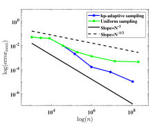
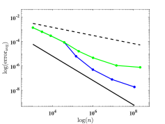
When uniform refinement and fixed low-degree element-wise interpolation are utilized, the number of elements is approximately , which indicates a convergence rate of . Furthermore, the decay rate remains only for the global polynomial interpolation method proposed in [51]. Hence, Algorithm 2 achieves at least triple convergence rate compared with the uniform refinement with the fixed low-degree interpolation (degree=2 in our numerical experiment), as well as the global polynomial interpolation method.
5 Numerical experiments and discussions
Now we apply Algorithm 2 to the design of 3D PhCs with wide band gaps. We take two cubic unit cells with lattice constant filled with air embedded with six silicon blocks and a central silicon sphere. The length, width and height of the blocks, and radius of the sphere are design variables. Although the assumption of a symmetric unit cell facilitates computation, a symmetry reduction of the unit cell can open wider band gaps or create new band gaps [20, 16, 17]. Thus, adding more design variables to describe an asymmetrical unit cell has great potential to maximize photonic band gaps. Algorithm 2 allows greatly reducing the associated high computational complexity. We utilize [9] to implement the iterative LEB algorithm involved in Algorithm 1.
5.1 Experimental setting
First we describe two experimental settings, denoted as Model 1 and Model 2 below.
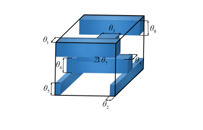
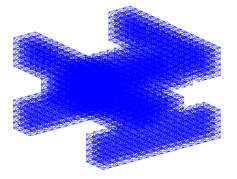
Model 1.
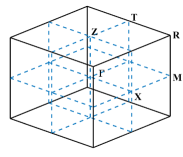
There are six silicon blocks layered inside a cubic unit cell , cf. Fig. 1(a) [33]. The relative permittivity inside the silicon blocks is . Their arrangement leads to -plane symmetry within the unit cell, but there is no symmetry along the -axis. The first Brillouin zone is shown in Fig. 1(b), where the high-symmetry points are denoted as . The IBZ is the polyhedron formed by connecting these high-symmetry points. This type of structure has been successfully applied in preclinical studies [39]. There are eight design parameters , cf. Fig. 1(a). We fix the block thickness as and only seek the optimal parameters to maximize the band gap over the admissible set
It is known that there is a band gap between 4th and 5th bands when and [6]. Note that the commonly used path to characterize the band function is insufficient to accurately detect band gaps. We will adaptively generate sampling points in the IBZ by Algorithm 1 and approximate band functions element-wisely by Algorithm 2.
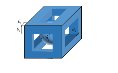
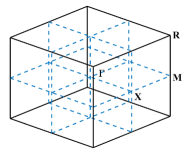
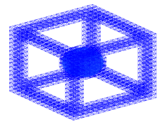
Model 2.
The unit cell also contains silicon blocks, cf. Fig. 1(c). Additionally, there is a silicon sphere with a radius of at the center of the unit cell. This structure imparts symmetry to the unit cell along the and axes. Therefore, the high-symmetry points in are , , and , and the region enclosed by the lines connecting them represents IBZ. This photonic crystal structure was fabricated in [34] by a sacrificial-scaffold mediated two-photon lithography strategy and using a degradable hydrogel scaffold. There are four design parameters , which are the dimensions (length and width) of the silicon blocks and the radius of the silicon sphere. We take the following admissible set
to ensure that there is no overlap between the silicon sphere and the silicon blocks. It can be verified experimentally that there is a band gap when and .
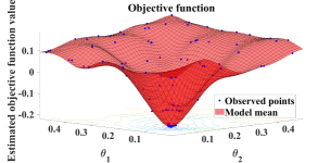
Next we formulate the band gap maximization problem as PDE constrained optimization. The objective is to determine the unit cell that maximizes the band gap, i.e., the distance between two adjacent band functions and . One intuitive way is to define the objective function by
| (5.1) |
with the design variable vector for shape-wise optimization. Usually, the objective function is normalized by the mean value in which the band gap is turned
| (5.2) |
which results in a modified objective function . We normalized the objective function to indicate how the band gap improves relative to the mean band gap frequency since it is crucial to know not only the band gap width but also its location.
Since each eigenfrequency is obtained by taking the square root of the eigenvalue in equation (2.5), we use the following objective function
In sum, the optimization problem can then be formulated as
| (5.3) |
subject to the following variational formulation with ,
Remark 5.1.
Typically, the unit cell chosen for optimization already possesses some band gaps under certain predefined parameters. For instance, given a specific set of parameters , there exists a band gap between the th and th band functions for Model 1, i.e., . Then we aim to solve (5.3) with . On the contrary, if the unit cell being optimized does not possess any a priori band gaps, we can use the following objective function,
| (5.4) |
It aims to find an optimal parameter that maximizes the band gap among the first band functions. By maximizing the difference between the minimum and maximum values of adjacent band functions within the Brillouin zone , we can effectively enhance the band gap therebetween.
Next we describe how to solving Problem (5.3), which is divided into two steps. The first step is to evaluate the objective function for a given parameter , which involves calculating and by Algorithm 2. The second step is to update the parameter from to to obtain a larger value in the objective function . One repeats these two steps until a certain criterion is attained. Note that solving (5.3) is challenging since it is non-convex and the derivatives of the objective function are neither symbolically nor numerically available. Thus, we adopt some derivative-free algorithms to deal with this problem (5.3). Bayesian optimization (BO) is a popular method for solving optimization problems involving expensive objective functions. Roughly speaking, BO uses a computationally cheap surrogate model to construct a posterior distribution over the original expensive objective using a limited number of observations. The statistics of the surrogate model are used to sample a new point where the original is then evaluated. The incorporation of such a surrogate model makes BO an efficient global optimization technique in terms of the number of function evaluations [41, 27, 47, 44]. To the best of our knowledge, the application of BO to photonic band gap maximization remains largely unexplored. In this work, we employ MATLAB’s built-in optimization solver bayesopt. We summarize the procedure in Algorithm 3. For more details about the BO algorithm, we refer to [27, 46].
5.2 Maximization of band gap
Now we solve (5.3) with , for Model 1, and , for Model 2 by Algorithm 2. We use the lowest order -modified Nédélec edge elements (2.9) and discretize the computational domain with a uniform mesh comprised of 24576 tetrahedral elements in Fig. 2(a) for Model 1, 24650 tetrahedral elements in Fig. 2(b) for Model 2. The employed mesh serves dual purposes: first, to fulfill periodic boundary conditions, ensuring a one-to-one correspondence of edges along opposing faces of the cubic domain; second, for Model 2, the tetrahedral mesh necessitates partitioning along the spherical material situated at the center of the cubic domain.
Now we describe the initialization strategy for Algorithm 3.
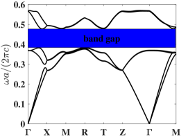
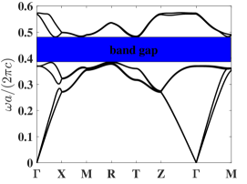
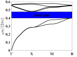
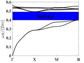
(i): Model 1. The band structure of the cubic lattice with lattice constant , and design variables is initially computed. The resulting band structure shows a band gap between the th and th bands with normalized band gap width . The first six band functions along the high symmetry points are shown in Fig. 3(a). Although there is already a band gap in the initial structure, band gap optimization facilitates a deeper understanding of how their sizes can affect the band gap via parameter optimization.
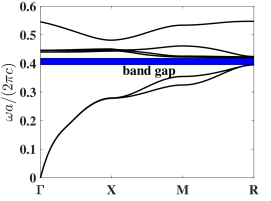
(ii): Model 2. In case , , PhCs with such a unit cell can forbid certain frequencies of light. We consider optimizing these four parameters with silicon blocks and sphere inside the unit cell to find a nearly optimal band gap range. The band structure with initial configuration is computed and the resulting band structure shows a band gap between the nd and rd bands with normalized band gap width . The first six band functions along the high symmetry points are shown in Fig. 3(b).
Next we describe the optimization results of normalized band gap (5.3).
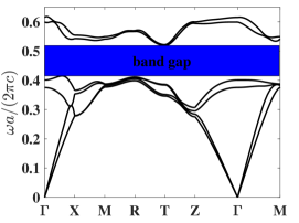
For Model 1, we first fix and only optimize , which denotes the width of the four blocks on the 1st and 4th layers. The outcome is shown in Fig. 4(a). Several iterations of Algorithm 3 generate a set of parameters with their band gaps being larger than the known band gap. The optimal values we obtain is and the maximal normalized band gap is . This optimization process generates a larger band gap compared to existing literature where the design variables are chosen to be and the corresponding normalized band gap is . For the optimized parameter, the bandgap width increases by . Further, we optimize parameters simultaneously. The results show that when , one obtains a unit cell design with a larger band gap than the one in the literature. The band gap of the configuration is , which is higher than the original one. The first six band functions, under these two new sets of design parameters, along the high symmetry points are shown in Fig. 5.
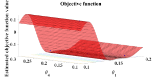
For Model 2, we first consider blocks of square cross-section, i.e. in 1(c) to get a visualized optimization process in Figure 4(b). In this case, Algorithm 3 produces a set of parameters such that the band gap is larger than that of the configuration in reference [34] after a few iterations of parameter selection. The optimal parameters are with the normalized band gap is , which is higher than the original band gap. Next we optimize parameters independently. The results show that yields a unit cell design with a much larger band gap than the one reported in the literature. The band gap of the configuration is , which is higher than the original band gap. The first six band functions along the high symmetry points under these two sets of design parameters are depicted in Fig. 6.
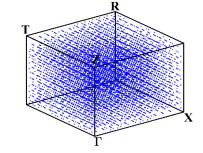
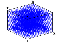
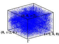
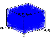
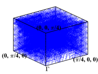
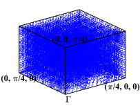
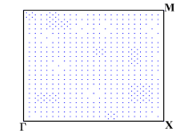
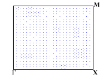
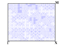
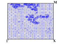
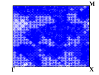
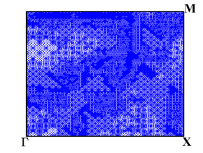
During the optimization process, for any generated ”next point”, we adaptively select the sampling points in the first Brillouin zone and element-wisely interpolate and . During these four optimization processes, we performed 8 loops of adaptive mesh refinement under each set of parameters. Fig. 7 shows the points used to approximate the objective function under the optimal parameters. We observe that the distribution of the sampling points is not uniform.
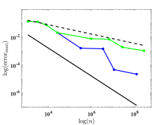
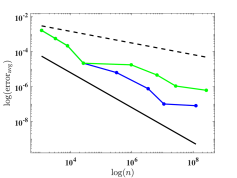
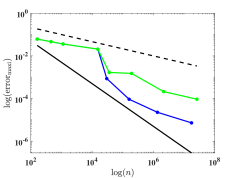
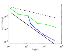
5.3 Efficiency of Algorithm 2
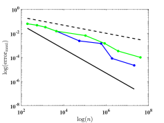
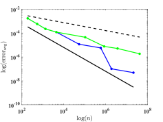
Finally, we show the efficiency of Algorithm 2 by comparing with uniform mesh refinement with lowest-order element-wise interpolation under the optimal parameters. In both models, we randomly choose 5000 -points in the IBZ (denoted by ), on which we compute the reference solution using the -conforming -modified Nédélec edge FEM (2.9) with the mesh in Fig. 2. The pointwise relative error is then computed on by
for some certain band number . Here, is the th reference band function obtained directly by the -conforming -modified Nédélec edge FEM using the same mesh on the unit cell , and is obtained by the element-wise polynomial interpolation. We measure the accuracy of the methods using maximum and average relative errors
where , for Model 1 and for Model 2.
We depict in Fig. 7 the distribution of the sampling points for Model 1 with four optimizing parameters obtained from Algorithm 1. We observe that the sampling points are not uniformly distributed. Moreover, Fig. 8 presents the relative errors with respect to the number of sampling points, where and versus , i.e., the number of sampling points, on log-log coordinates with and are plotted. We observe that Algorithm 2 has a much faster convergence rate than the uniform one. Further, compared with the reference lines, Algorithm 2 has an approximately first-order convergence rate, while the uniform method is much less efficient with an approximately -order convergence rate, which is consistent with Theorem 4.6 and Remark 4.1.
6 Conclusions
In this work, we present a generalization of an -adaptive sampling method for computing the band functions of three-dimensional photonic crystals with an application in the band gap maximization. We present theoretical analysis and numerical tests to verify its performance. For the band gap maximization problem, we generate an adaptive mesh in the parameter domain each time when the geometry of the photonic crystal is updated. One intriguing question is whether one can use the same adaptive mesh for a few updates in the geometry of the photonic crystals in order to make our algorithm more efficient. Also, it is of interest to have more freedom in constructing photonic crystals with an infinite number of design parameters, e.g., the interface between two different materials can be designed.
References
- [1] I. Babuška and M. Suri. The and versions of the finite element method, basic principles and properties. SIAM Rev., 36(4):578–632, 1994.
- [2] Z. Bai, J. Demmel, J. Dongarra, A. Ruhe, and H. van der Vorst. Templates for the Solution of Algebraic Eigenvalue Problems: a Practical Guide. SIAM, Philadelphia, PA, 2000.
- [3] M. Blyth and C. Pozrikidis. A Lobatto interpolation grid over the triangle. IMA J. Appl. Math., 71(1):153–169, 2006.
- [4] D. Boffi, M. Conforti, and L. Gastaldi. Modified edge finite elements for photonic crystals. Numer. Math., 105:249–266, 2006.
- [5] D. Boffi, P. Fernandes, L. Gastaldi, and I. Perugia. Computational models of electromagnetic resonators: analysis of edge element approximation. SIAM J. Numer. Anal., 36(4):1264–1290, 1999.
- [6] A. Bulovyatov. A parallel multigrid method for band structure computation of 3D photonic crystals with higher order finite elements. PhD thesis, Karlsruhe Institute of Technology, Karlsruhe, 2010.
- [7] J. Chan and T. Warburton. A comparison of high order interpolation nodes for the pyramid. SIAM J. Sci. Comput., 37(5):A2151–A2170, 2015.
- [8] F. Chen, S. Wang, and H. Nasrabadi. Molecular simulation of competitive adsorption of hydrogen and methane: Analysis of hydrogen storage feasibility in depleted shale gas reservoirs. In SPE Reservoir Simulation Conference. OnePetro, 2023.
- [9] L. Chen. FEM: an integrated finite element methods package in MATLAB. Technical report, 2009.
- [10] Y. Chen, Z. Lan, and J. Zhu. Inversely designed second-order photonic topological insulator with multiband corner states. Phys. Rev. Appl., 17(5):054003, 2022.
- [11] S.-H. Chou, T.-M. Huang, T. Li, J.-W. Lin, and W.-W. Lin. A finite element based fast eigensolver for three dimensional anisotropic photonic crystals. J. Comput. Phys., 386:611–631, 2019.
- [12] A. Chutinan, S. John, and O. Toader. Diffractionless Flow of Light in All-Optical Microchips. Phys. Rev. Lett., 90(4):123901, 2003.
- [13] R. Craster, T. Antonakakis, M. Makwana, and S. Guenneau. Dangers of using the edges of the Brillouin zone. Phys. Rev. B, 86(11):115130, 2012.
- [14] C. Dobson, J. Gopalakrishnan, and E. Pasciak. An efficient method for band structure calculations in 3D photonic crystals. J. Comput. Phys., 161(2):668–679, 2000.
- [15] C. Dobson and E. Pasciak. Analysis of an algorithm for computing electromagnetic Bloch modes using Nédélec spaces. Comput. Methods Appl. Math., 1(2):138–153, 2001.
- [16] H.-W. Dong, X.-X. Su, Y.-S. Wang, and C. Zhang. Topology optimization of two-dimensional asymmetrical phononic crystals. Phys. Lett. A, 378(4):434–441, 2014.
- [17] H.-W. Dong, Y.-S. Wang, Y.-F. Wang, and C. Zhang. Reducing symmetry in topology optimization of two-dimensional porous phononic crystals. Aip Adv., 5(11), 2015.
- [18] L. Dong, A. Mckay, A. Marcinkevicius, L. Fu, J. Li, K. Thomas, and E. Fermann. Extending effective area of fundamental mode in optical fibers. J. Lightwave Technol., 27(11):1565–1570, 2009.
- [19] T. Eidam, J. Rothhardt, F. Stutzki, F. Jansen, S. Hädrich, H. Carstens, C. Jauregui, J. Limpert, and A. Tünnermann. Fiber chirped-pulse amplification system emitting 3.8 GW peak power. Optics Expr., 19(1):255–260, 2011.
- [20] A. Gazonas, S. Weile, R. Wildman, and A. Mohan. Genetic algorithm optimization of phononic bandgap structures. Int. J. Solids Struct., 43(18-19):5851–5866, 2006.
- [21] I. M. Glazman. Direct Methods of Qualitative Spectral Analysis of Singular Differential Operators. Israel Program for Scientific Translations, 1965.
- [22] M. Hammond, A. Oskooi, M. Chen, Z. Lin, G. Johnson, and E. Ralph. High-performance hybrid time/frequency-domain topology optimization for large-scale photonics inverse design. Optics Expr., 30(3):4467–4491, 2022.
- [23] J. Harrison, P. Kuchment, A. Sobolev, and B. Winn. On occurrence of spectral edges for periodic operators inside the Brillouin zone. J. Phys. A: Math. Theor., 40(27):7597, 2007.
- [24] W.-Q. Huang, W.-W. Lin, H.-S. Lu, and S.-T. Yau. iSIRA: Integrated shift–invert residual Arnoldi method for graph Laplacian matrices from big data. J. Comput. Appl. Math., 346:518–531, 2019.
- [25] D. Jackson. Classical Electrodynamics. American Association of Physics, New York, 1999.
- [26] J. D. Joannopoulos, S. G. Johnson, J. N. Winn, and R. D. Meade. Photonic Crystals: Molding the Flow of Light. Princeton Univ. Press, Princeton, NJ, 2008.
- [27] R. Jones, M. Schonlau, and J. Welch. Efficient global optimization of expensive black-box functions. J. Global optim., 13:455–492, 1998.
- [28] P. Kuchment. Floquet Theory for Partial Differential Equations. Springer, Basel, 1993.
- [29] D. Labilloy, H. Benisty, C. Weisbuch, T. Krauss, V. Bardinal, and U. Oesterle. Demonstration of cavity mode between two-dimensional photonic-crystal mirrors. Elec. Lett., 33(23):1978–1980, 1997.
- [30] V. Laude. Phononic Crystals. de Gruyter, Berlin/Boston, 2002.
- [31] J.-F. Lee, D. Sun, and Z. Cendes. Tangential vector finite elements for electromagnetic field computation. IEEE Trans. Magnet., 27(5):4032–4035, 1991.
- [32] H. Li, G. Ren, Y. Gao, B. Zhu, J. Wang, B. Yin, and S. Jian. Hollow-core photonic bandgap fibers for orbital angular momentum applications. J. Optics, 19(4):045704, 2017.
- [33] S.-y. Lin, J. Fleming, D. Hetherington, B. Smith, R. Biswas, K. Ho, M. Sigalas, W. Zubrzycki, S. Kurtz, and J. Bur. A three-dimensional photonic crystal operating at infrared wavelengths. Nature, 394(6690):251–253, 1998.
- [34] K. Liu, H. Ding, S. Li, Y. Niu, Y. Zeng, J. Zhang, X. Du, and Z. Gu. 3d printing colloidal crystal microstructures via sacrificial-scaffold-mediated two-photon lithography. Nature Comm., 13(1):4563, 2022.
- [35] Z. Lu, A. Çesmelioglu, J. Van der Vegt, and Y. Xu. Discontinuous Galerkin approximations for computing electromagnetic Bloch modes in photonic crystals. J. Sci. Comput., 70(2):922–964, 2017.
- [36] Z. Lu and Y. Xu. A parallel eigensolver for photonic crystals discretized by edge finite elements. J. Sci. Comput., 92(3):79, 2022.
- [37] H. Luo and C. Pozrikidis. A Lobatto interpolation grid in the tetrahedron. IMA J. Appl. Math., 71(2):298–313, 2006.
- [38] X.-l. Lyu, T. Li, T.-m. Huang, J.-w. Lin, W.-w. Lin, and S. Wang. FAME: fast algorithms for Maxwell’s equations for three-dimensional photonic crystals. ACM Trans. Math. Software (TOMS), 47(3):1–24, 2021.
- [39] J. Mačiulaitis, M. Deveikytė, S. Rekštytė, M. Bratchikov, A. Darinskas, A. Šimbelytė, G. Daunoras, A. Laurinavičienė, A. Laurinavičius, R. Gudas, et al. Preclinical study of SZ2080 material 3D microstructured scaffolds for cartilage tissue engineering made by femtosecond direct laser writing lithography. Biofabrication, 7(1):015015, 2015.
- [40] F. Maurin, C. Claeys, E. Deckers, and W. Desmet. Probability that a band-gap extremum is located on the irreducible Brillouin-zone contour for the 17 different plane crystallographic lattices. Int. J. Solids Struct., 135:26–36, 2018.
- [41] J. Mockus. Application of Bayesian approach to numerical methods of global and stochastic optimization. J. Global Optim., 4:347–365, 1994.
- [42] M. Rivara and C. Levin. a 3-d refinement algorithm suitable for adaptive and multi-grid techniques. Comm. Appl. Numer. Methods, 8:281–290, 1992.
- [43] P. Russell. Photonic crystal fibers. Science, 299(5605):358–362, 2003.
- [44] J. Sasena. Flexibility and efficiency enhancements for constrained global design optimization with kriging approximations. University of Michigan, Ann Arbor, Michigan, 2002.
- [45] C. Schwab. -and -Finite Element Methods: Theory and Applications in Solid and Fluid Mechanics. Oxford University Press, Oxford, 1998.
- [46] B. Shahriari, K. Swersky, Z. Wang, P. Adams, and N. De Freitas. Taking the human out of the loop: A review of Bayesian optimization. Proceedings of the IEEE, 104(1):148–175, 2015.
- [47] S. Streltsov and P. Vakili. A non-myopic utility function for statistical global optimization algorithms. J. Global Optim., 14:283–298, 1999.
- [48] D. Sun, J. Manges, X. Yuan, and Z. Cendes. Spurious modes in finite-element methods. IEEE Antennas Prop. Mag., 37(5):12–24, 1995.
- [49] S. Wang, S. Li, and Y.-S. Wu. An analytical solution of pressure and displacement induced by recovery of poroelastic reservoirs and its applications. SPE J., 28(03):1329–1348, 2023.
- [50] Y. Wang and G. Li. An -adaptive sampling algorithm on dispersion relation reconstruction for 2D photonic crystals. arXiv preprint, arXiv:2311.16454, 2023.
- [51] Y. Wang and G. Li. Dispersion relation reconstruction for 2D photonic crystals based on polynomial interpolation. J. Comput. Phys., 498:112659, 2024.
- [52] A. Woldering, P. Mosk, and L. Vos. Design of a three-dimensional photonic band gap cavity in a diamondlike inverse woodpile photonic crystal. Phys. Rev. B, 90(9):115140, 2014.
- [53] Y. Yan, P. Liu, X. Zhang, and Y. Luo. Photonic crystal topological design for polarized and polarization-independent band gaps by gradient-free topology optimization. Optics Expr., 29(16):24861–24883, 2021.
- [54] F. Yanik, S. Fan, M. Soljačić, and D. Joannopoulos. All-optical transistor action with bistable switching in a photonic crystal cross-waveguide geometry. Optics Lett., 28(24):2506–2508, 2003.