An extremal problem arising in the dynamics of two-phase materials that directly reveals information about the internal geometry
2Department of Mathematics, University of Utah, Salt Lake City, UT 84112, USA,
3Department of Mathematics, University of California at Santa Barbara, CA 93106, USA, and School of Mathematics, Statistics and Physics, Newcastle University, NE1 7RU Newcastle upon Tyne, UK.
Emails: [email protected], [email protected], [email protected], [email protected])
Abstract
In two phase materials, each phase having a non-local response in time, it has been found
that for some driving fields the response somehow untangles at specific times, and
allows one to directly infer useful information about the geometry of the material, such as
the volume fractions of the phases. Motivated by this, and to obtain an algorithm for designing
appropriate driving fields, we find approximate, measure independent, linear relations between the
values that Markov functions take
at a given set of possibly complex points, not belonging to the interval [-1,1] where the measure
is supported.
The problem is reduced to simply one of polynomial approximation of a given
function on the interval [-1,1] and to simplify the analysis Chebyshev approximation is used.
This allows one to obtain explicit estimates of the error of the approximation, in terms
of the number of points and the minimum distance of the points to the interval [-1,1].
Assuming this minimum distance is bounded below by a number greater than 1/2, the error
converges exponentially to zero as the number of points is increased. Approximate linear relations
are also obtained that incorporate a set of moments of the measure. In the context of the
motivating problem, the analysis also yields bounds on the response at any particular time
for any driving field, and allows one to estimate the response at a given frequency using an
appropriately designed driving field that effectively is turned on only for a fixed interval of
time. The approximation extends directly to Markov-type functions with a positive semidefinite
operator valued measure, and this has applications to determining the shape of an inclusion
in a body from boundary flux measurements at a specific time, when the time-dependent
boundary potentials are suitably tailored.
Keywords: Composites, best rational approximation, volume fraction estimation, bounds on transient response, Calderon problem, Markov functions
1 Introduction
Many systems have responses that are nonlocal in time as this is naturally a consequence of the fact that it takes time for subelements of the system to respond. Usually, this leads one to either: (1) examine the response at each, or one or more, frequencies as the convolution in time characterizing the response of the system becomes a simple multiplication in the frequency domain; or (2) examine the response to a delta function or Heaviside function as this directly reveals the integral kernel characterizing the response. In this paper we show that desired information about the system can be directly obtained from selectively designed input signals that are neither at constant frequency, nor delta or Heaviside functions.
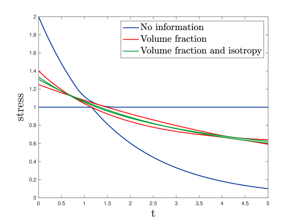
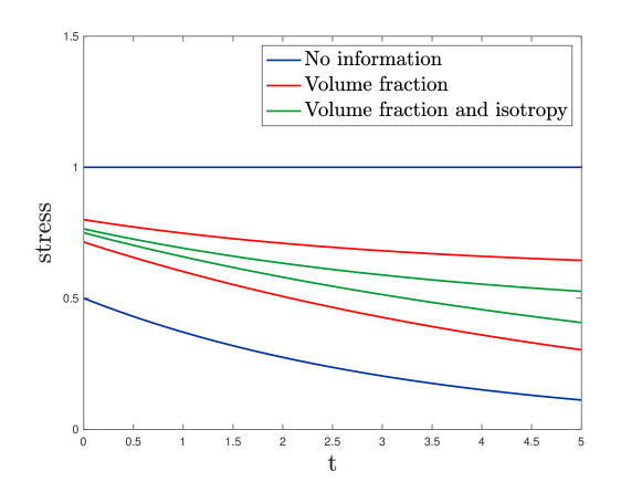
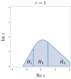
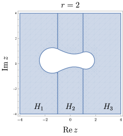
Our initial motivation comes from the work [31, 33] where we derived microstructure-independent bounds on the viscoelastic response at a given time of two-phase periodic composites (in antiplane shear) with prescribed volume fractions and of the phases and with an applied average stress or strain prescribed as a function of time. We found that the bounds were sometimes extremely tight at particular times : see Figure 1. This was quite a surprise because the response of each phase is nonlocal in time, yet somehow this response is untangled at these particular times. Thus, the bounds could be used in an inverse fashion to determine the volume fractions from measurements at time . Determining volume fractions of phases is important in the oil industry, where one wants to know the proportions occupied by oil and water in the rock, to detecting breast cancer, to assessing the porosity of sea-ice and other materials, and even to determining the volume of holes in swiss cheese. While our bounds were very tight at specific times in some examples, they were far from tight at all times in other examples: see Figure 2.
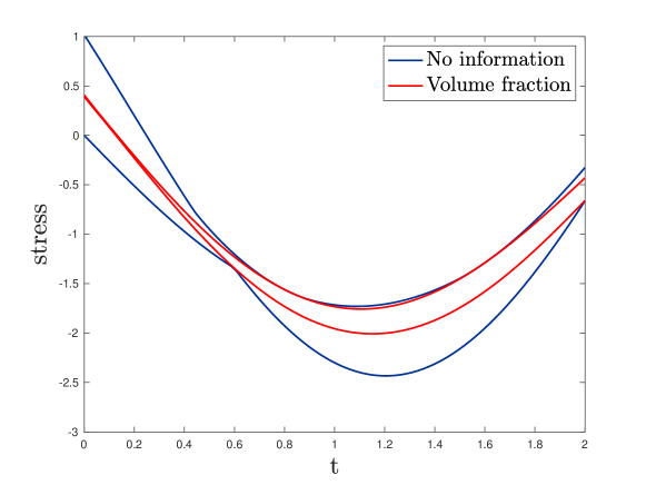
At that time it was totally unclear as to whether appropriate input signals could produce the desired tight bounds at a specific time and, if so, what algorithm should be followed to design these input signals. The primary goal of this paper is to address this problem in the case where the input function has a finite number of frequencies. In particular, for the example of Figure 2, our algorithm produces the much tighter bounds of Figure 3. It is an open question as to whether one can find smooth input signals, containing a continuum of frequencies, such that the response of the material at a specific moment of time is totally measure independent, while has a smooth dependence on , with when . The example of Figure 1 suggests that it may be possible.
We emphasize that our results are applicable not just to determining the volume fractions of the phases in a two-phase composite but also determining the volume and shape of an inclusion in a body from exterior boundary measurements. This is shown in Sections 10 and 11. It is a classical and important inverse problem with a long history and many contributions: see [10, 26, 27, 47, 46, 22, 1, 19, 9, 11, 4, 3, 25, 44, 28] and references therein.
A secondary goal of this paper is to solve an accompanying mathematical approximation problem which we now outline, and which is essential to achieve the primary goal.
2 A fundamental mathematical question of approximation applicable to Markov functions
Here we formulate a problem, not just relevant to systems with a nonlocal response, but potentially to other application where Markov functions arise. Such functions are Cauchy transforms of positive measures with compact support on the real line. Some authors may suitably call them Herglotz functions, or Nevanlinna functions, or Stieltjes transforms.
Suppose is a Markov function having the integral representation
| (2.1) |
where the Borel measure is positive with unit mass:
| (2.2) |
Given (possibly complex) points not belonging to the interval , we are interested in finding complex constants such that
| (2.3) |
for all probability measures . Optimal bounds correlating the possible values of the -tuple as varies over all probability measures are well known, as derived from the well charted analysis of the Nevanlinna-Pick interpolation problem [29]. Indeed, the nonlinear constraints among the values , and standard convexity theory provide optimal bounds on the range of the left hand side of (2.3) for given constants , see [29] for details. But this is not our main concern.
We would rather like to choose points , and find associated constants , for every prescribed integer , having the property
| (2.4) |
for some bound subject to as . The geometry of the locus of these points is obviously essential and it will be detailed in the sequel. The faster the convergence, the better.
Since we deal with probability measures, condition (2.4) is equivalent to
| (2.5) |
And this is good news. We seek the minimal deviation from zero on the interval of a rational function satisfying and possessing simple poles at the points . Or equivalently, denoting and we aim at finding the minimal deviation from zero of a monic polynomial of degree , with respect to the weighted norm
Both perspectives align to well-known classical studies in approximation theory. The first one is an extremal problem in rational approximation with prescribed poles, a subject going back at least to Walsh [51]. A great deal of information in this respect was systematized in Walsh’s book [52]. The second approach is a genuine weighted Chebyshev approximation problem, and here we are on solid ground. First, note that the functions
| (2.6) |
form a Chebyshev system on the interval , that is, they are linearly independent and any linear combination of has at most zeros in . Even more, a stronger so-called Markov property of this system of functions holds. The classical Chebyshev approximation in the uniform norm theorem has an analog for such non-orthogonal bases [23, 29]. To be more precise, there exists a unique monic polynomial of degree minimizing the norm : this polynomial is characterized by the fact that attains its maximal value at points, and the sign of alternates there, see also [34]. In case , the optimal polynomial is of course the normalized Chebyshev polynomial of the first kind: The constructive aspects of weighted Chebyshev approximation are rather involved, see for instance the early works of Werner [54, 55, 56]. In the same vein, the asymptotics of the optimal bound of our minimization problem inherently involves potential theory or operator theory concepts. We cite for a comparison basis a few remarkable results of the same flavor [16, 45, 6].
Without seeking sharp bounds and guided by the specific applications we aim at, we propose a compromise and relaxation of our extremal problem:
| (2.7) |
At this point we can invoke Chebyshev original theorem and his polynomial , obtaining in this way the benefit, very useful for applications, of computing in closed form the residues . Details and some ramifications will be given in the Section 4.
3 Relevance of the approximation problem to systems with a non-local time response and the viscoelasticity problem in particular.
Without going into the specific details, as these will be provided later in Section 7, 8 and 9, in many linear systems with an input function varying with time , of the form
| (3.1) |
where the are a set of (possibly complex) frequencies, and is a given time, the output function takes the form
| (3.2) |
in which the function is given by (2.1),
| (3.3) |
and the functions and depend on in some known way: and . The real constant and the unknown measure depend on the system. In our viscoelasticity study [33] the connection with Markov functions comes from the fact that the effective shear modulus , that relates the average stress to the average strain at frequency , as a function of the shear moduli and of the two phases, has the property that , in which is the volume fraction of phase 1, is a Markov function of taking the form (2.2) [7, 35, 15].
Henceforth, we adopt the notational simplification
Thus, at time , the output function is
| (3.4) |
and we seek an input signal so that the output is almost system independent with . So, by measuring we can determine the system parameter . In the viscoelastic problem that we studied [31, 33], is the volume fraction (see also [7]) and it is useful to be able to determine this from indirect measurements. Typically, one may assume the frequencies have a positive imaginary part so that the input signal is essentially zero in the distant past. In (3.1) one could just take a signal with frequencies , . Then, we have
| (3.5) |
Then, if is known, a measurement of will allow us to estimate the output at a desired (possibly real) frequency given the time harmonic input .
It is often the situation, such as in the viscoelastic problem, that only the real part of has a direct physical significance and, hence, one might want to find constants such that, say,
| (3.6) |
where the overline denotes complex conjugation. This, again, reduces to a problem of the form (2.3) where, after renumbering, the complex values of come in pairs, and and we may take so that the left hand side of (2.3) is real.
It may be the case that the first moments of the probability measure are known,
| (3.7) |
in addition to the zeroth moment and that (possibly complex) points not on the interval are given. We then may seek complex constants and , with say , such that
| (3.8) |
for all probability measures with the prescribed moments. We will treat this problem in Section 3. We can use these results to determine an approximate linear relation among the moments if is measured. This may be used to estimate one moment if the rest are known. This can be useful when the moments have an important physical significance: in the viscoelastic problem, for instance, depends only on the volume fraction if one assumes that the composite has sufficient symmetry to ensure that its response remains invariant as the material is rotated [7]. So, incorporating the moment and measuring the response at time , then, allows us to obtain tighter bounds on as shown in [31, 33].
Mutatis mutandis, we may seek complex constants and (each constant depending both on and ) such that
| (3.9) |
where the infimum is over all self adjoint operators with spectrum in and for fixed , as . Our analysis extends easily to treat this problem too. The relevance is that in many linear systems with an input field varying with time , of the form
| (3.10) |
the output field takes the form
| (3.11) |
where the real constant and the self-adjoint operator characterize the response of the system, and the system parameters and depend on the frequency in some known way. Then, the bound (3.9) implies
| (3.12) |
4 The solution to the main approximation problem
The present section contains the main result which provides the theoretical foundation of our explorations. As explained in the introduction, we try to balance the computational accessibility and simplicity with the loss of sharp bounds. A few comments about the versatility of the following theorem are elaborated after its proof.
Theorem 1
Letting
| (4.1) |
denote the distance from to the line segment , and assuming
| (4.2) |
one can find complex constants each depending on , such that (2.4) holds with as . In particular, with
| (4.3) |
where is the Chebyshev polynomial of the first kind, of degree ,
(2.4) holds with which tends to zero as .
Proof
We have
| (4.4) |
Since the right hand side of (4.4) is linear in its maximum over all probability measures is achieved when is an extremal measure, namely the point mass
| (4.5) |
where is varied in so as to get the maximum value of the right hand side of (4.4). In fact, for this extreme measure one has equality in (4.4). Equivalently, we have
| (4.6) | |||||
Thus, we seek a set of constants (each dependent on ) and sequence such that as and
| (4.7) |
More clearly, direct substitution of (4.7) into (4.4) shows that (2.4) holds.
Now we may write
| (4.8) |
where is the known monic polynomial
| (4.9) |
of degree , and is a polynomial of degree at most that remains to be determined. The constants can then be identified with the residues at the poles of :
| (4.10) |
Then, the problem becomes one of choosing such that
| (4.11) |
is close to zero. Clearly, the problem is now one of polynomial approximation of the monic polynomial of degree by the polynomial . A natural choice is to take
| (4.12) |
where is the Chebyshev polynomial of degree , normalized to be monic. This choice minimizes the sup-norm of over the interval and
| (4.13) |
provides a bound on the numerator in (4.11). To bound the denominator, we have
| (4.14) |
where is given by (4.1). Using (4.2) and the bounds (4.13) and (4.14) we see that (2.4) is satisfied with
. Finally, with given by (4.12) we see that the residues at the poles of , given
by (4.10) correspond to those given by (4.3).
Remark 1
The use of Chebyshev polynomials is convenient as bounds on their sup-norm over the interval are readily available. An alternative approach, also accessible from the numerical/computational point of view, is to work with the norm and find the polynomial of degree that approximates the given monic polynomial of degree in the precise sense that
| (4.15) |
is minimized. Subsequently, one has to invoke Bernstein-Markov’s inequality which bounds an norm by uniform norm.
This first step is a standard problem in the theory of orthogonal polynomials: one chooses to be the monic polynomial of degree that is
orthogonal to all polynomials of degree at most with respect to the measure . Separating the contribution of the denominator, by selecting to be the measure
we recover the Chebyshev polynomials we have advocated in the proof of the main result.
Remark 2
Assumption (4.2) is more than we really need. To underline the dependence on of all data we set
and
For the proof of Theorem 1 above we only need
That is, there exists , so that for large , the inequality
holds true.
By taking the natural logarithm, we are led to enforce the condition
In other terms, an evenly distributed probability mass on the points
should have its logarithmic potential asymptotically bounded from above by a prescribed constant, on the
interval . Again, this turns out to be a rather typical problem of approximation theory, at least when restricting
the poles of to belong to some Jordan curve surrounding . A natural choice being an ellipse with foci at , see also [45, 6].
Remark 3
We can gain more flexibility in the choice of the input signal if we replace in the formula (4.3) for the residues with , where is a prescribed (possibly complex) zero of . In particular, we may choose to, say, minimize
| (4.16) |
to help ensure that the output signal is not too wild. If we are only interested in so that the come in complex conjugate pairs, then we may replace in (4.3) with , and choose to, say, minimize
| (4.17) |
In the first case, note that the signal (3.1) is linear in while in the second case it is linear in the real coefficients of the quadratic . So in either case we have a linear space of possible signals (though should not be too large for the approximation to hold at time ). Also as so in this limit the frequency is absent from the input and output signals. More generally, to help minimize (4.16) or (4.17) one might replace with where is a polynomial of fixed degree .
5 Incorporating moments of the measure
Here we assume that the first moments of the probability measure , given by (2.1), are known, in addition to and that (possibly complex) points not on the interval are given. We seek complex constants and , with say such that
| (5.1) |
is small for all probability measures with the prescribed moments. The analysis proceeds as before, only now we introduce the polynomial
| (5.2) |
and set and to be the polynomials defined by (4.8) and (4.9). The goal is now to choose polynomials and of degrees and , respectively, such that is monic and
| (5.3) |
is close to zero. We choose and such that
| (5.4) |
This is simply the Euclidean division of the normalized Chebyshev polynomial by with being identified as the quotient polynomial and being identified as the remainder polynomial. Then, assuming (4.2) and using (4.14), we have
| (5.5) |
satisfying as , with being fixed. With constants given by (4.10) and constants being the coefficients of the polynomial , as in (5.2), it follows that
| (5.6) | |||||
Remark
The results exposed in the previous sections extend immediately to the resolvent case using the spectral representation
| (5.7) |
where is the spectrum of , assumed to be contained in the interval and is an orthogonal projection valued measure satisfying
| (5.8) |
Then, we have
| (5.9) | |||||
Choosing constants and , with , as in the previous section, the bound (5.5) substituted in (5.9) implies that the desired bound (3.9) holds with .
6 Bounds on the output function at any time
Supposing any constants are given, it is easy to get bounds on given by (3.2) at any time that incorporate the known moments . One introduces an angle and Lagrange multipliers and takes the minimum value of
| (6.1) |
as varies over all probability measures supported on with unconstrained moments. The minimum will be achieved by the point masses , where may take one or more values. Typically we will need to choose the Lagrange multipliers (that depend on ) so that the minimum is achieved at values , , and then adjust the measure to be distributed at these points
| (6.2) |
with the non-negative weights , that sum to , chosen so that the moments take their desired values. Then with this measure we obtain the bound
| (6.3) |
By varying from to we obtain bounds that confine to a convex region in the complex plane. Of course, if we are only interested in bounding , then it suffices to take or .
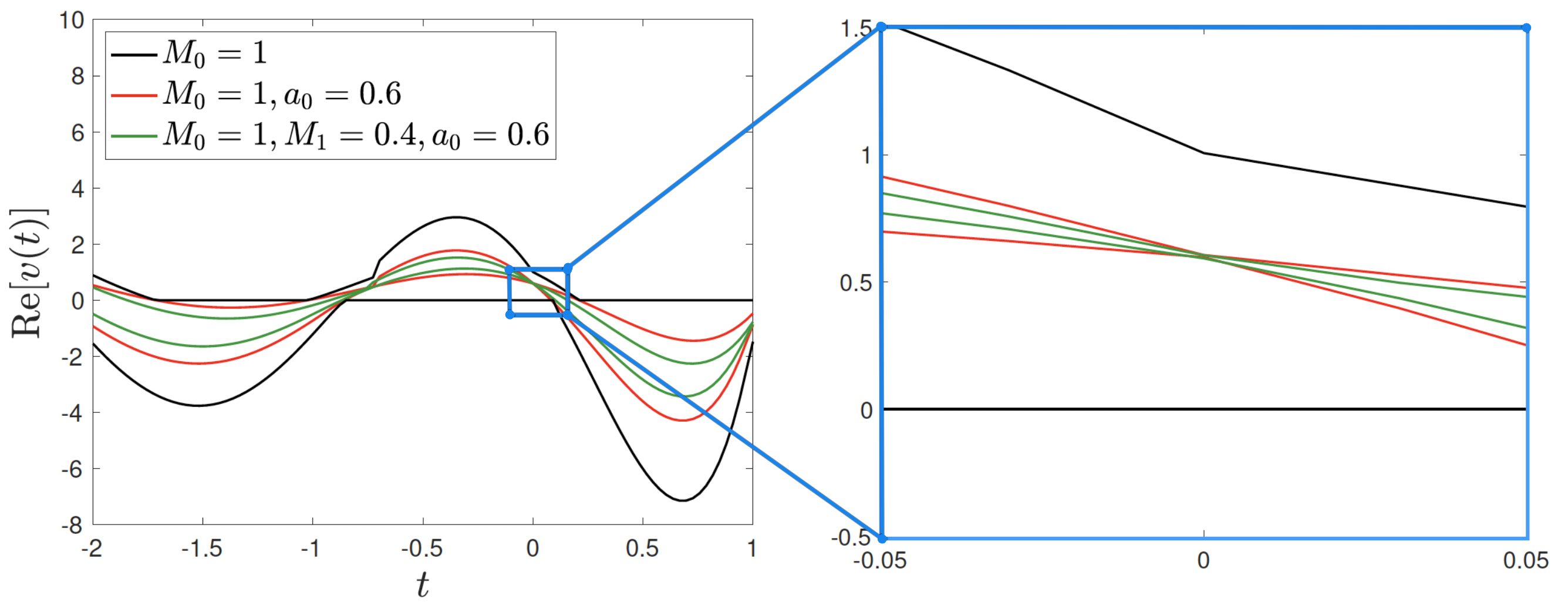
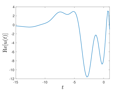
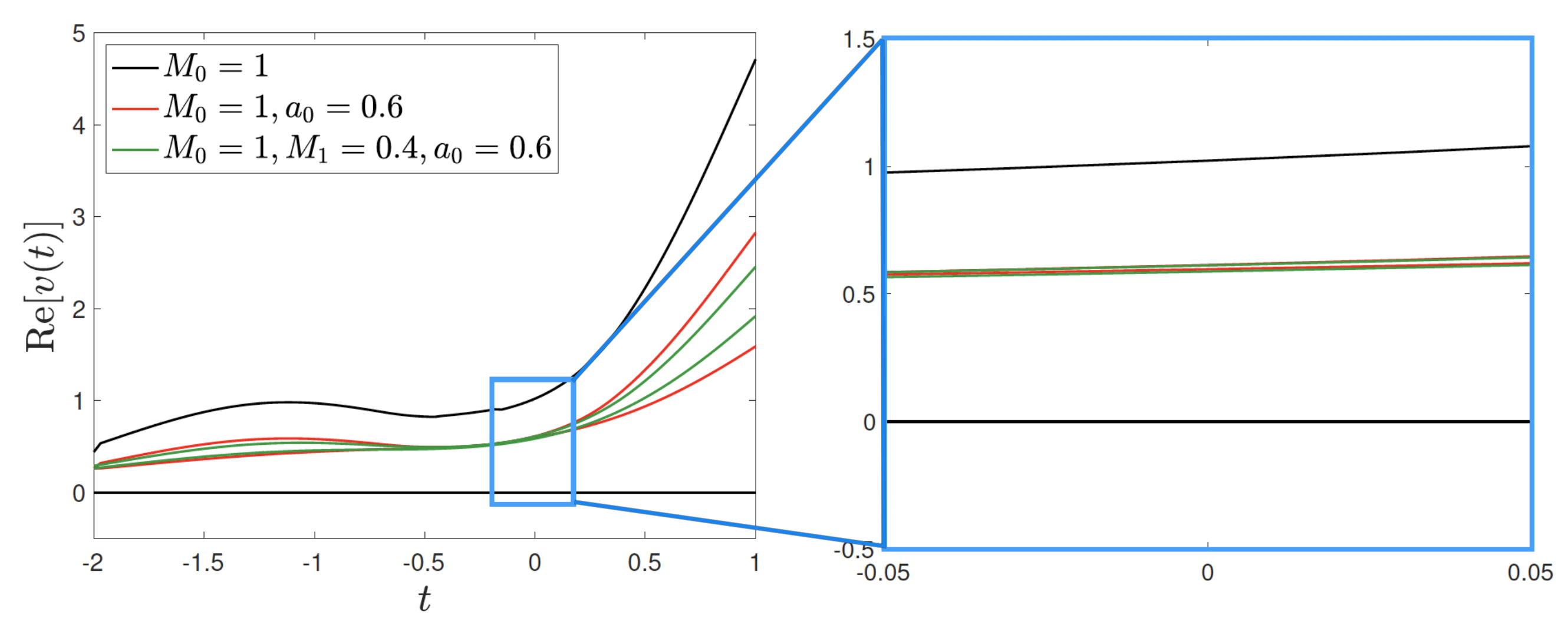
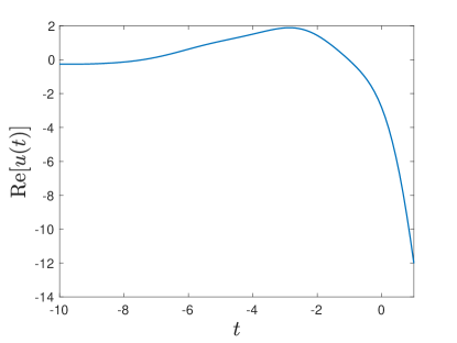
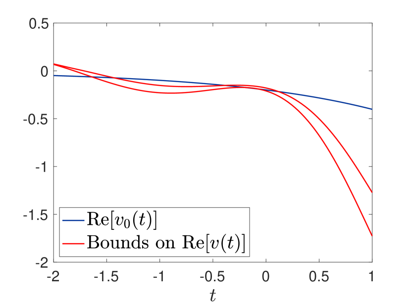
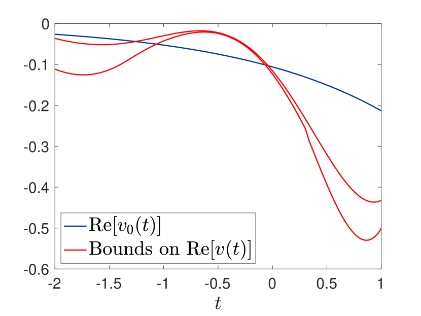
Figure 4 and Figure 5 depict the lower and upper bounds on for two systems ( in Figure 4, thus mimicking the low frequency dielectric response of a lossy dielectric material, and in Figure 5, thus mimicking the dielectric response of a plasma), when the coefficients in (6.3) are chosen such that the bounds are extremely tight at , according to (4.3). For both systems, the bounds on are tighter the higher the amount of pieces of information on the system is incorporated. Notice that the bounds colored in black (the largest ones) correspond to the case where only the zeroth order moment of the measure is known but not the value of : in such a case, as shown by the zoomed graph in the blue box, at , the upper bound takes value 1 and the lower bound takes value 0, that are the smallest and the highest values can take. On the other hand, when is assigned, the value that the corresponding bounds take at is exactly , as shown by the zoomed graph in the blue box. The graphs show clearly that, in order to estimate the system parameter , one has just to measure the response of the system at a specific moment of time (if the applied field is carefully chosen).
These are the type of bounds used in [33] to bound the temporal response of two-phase composites in antiplane elasticity. It is not yet clear whether those bounds can be derived from variational principles. In general, in the theory of composites, variational methods have proven to be more powerful than analytic approaches. Variational methods produce tighter bounds that often easily extend to multiphase composites: see the books [13, 49, 37, 2, 48] and references therein. For example, the variational approach gives tighter bounds on the complex permittivity at constant frequency of two-phase lossy composites [24], than the bounds obtained by the analytic approach [35, 8]. It also produces bounds on the complex effective bulk and shear moduli of viscoelastic composites [14, 42]. An exception is bounds that correlate the complex effective dielectric constant at more than two frequencies [36] that have yet to be obtained by a systematic variational approach. Variational bounds in the time domain are available [12, 32], but these are nonlocal in time.
7 Using an appropriate input signal to predict the response at a given frequency
Naturally, if one is interested in the response at a given (possibly complex) frequency , the easiest solution is to take an input signal at that frequency. However, it might not be easy to experimentally generate a signal at that frequency or it might not be easy to measure the response at that frequency. The problem becomes: find complex constants such that
| (7.1) |
with , . Defining the polynomials and as in (4.8) and (4.9) one needs to find of degree such
| (7.2) |
Proceeding as before we choose
| (7.3) |
where has been chosen so that the polynomial has a factor of . Then the residues of are given by
| (7.4) |
and
| (7.5) |
so that (7.1) holds with
| (7.6) |
where denotes the distance from to the interval [-1,1]. Joukowski’s map yields:
| (7.7) |
whence
| (7.8) |
Moreover, since runs over a circle of radius , we have
| (7.9) |
and
| (7.10) |
implying
| (7.11) |
All in all, the relevant bound satisfies
| (7.12) |
We obtain an exponential decay as provided the geometry of the loci is subject to the following condition: for a positive constant , each where
| (7.13) |
In other words, all of the must be close to in the precise sense that . Note that, as shown in Figure 6a, in case , and are sectors of disks, while is a portion of an ellipse. For these regions are complements of disks/ellipse, containing the point , as shown in Figure 6c. Some of these regions can be empty, depending on the position of .
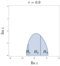
A conservative choice would be (see Figure 6b), in which situation and are bounded by straight lines, while is a parabola. To fix ideas, let us assume with and . All other cases being symmetrical. Then the euclidean region where are allowed consists of points subject to the constraints:
| (7.14) |
union with
| (7.15) |
If then necessarily and is simply the right-half plane , while in the case , is the interior of a parabola with vertex at , within the band , union with the polygonal region defined by the first distance inequality (in ).
Now with an input signal of the form (3.1), with , generating the output function given by (3.2), (7.1) implies the bound
| (7.16) |
where
| (7.17) |
is the response at time to the single frequency input signal
| (7.18) |
Of course, because this response is for a single frequency, determines for all .
In Figure 7 we depict the response of a given system subject to an input signal at the frequency and we compare the value it takes at with the value taken by the bounds on the response of a system having the same values of the moments of the measure but subject to a multiple-frequency signal with amplitudes chosen such that the bounds are extremely tight at : lies, as expected, between the bounds on at ,
Remark
The analysis is easily extended to the case where the response is known for a given but one wants to predict the derivative
| (7.19) |
As
| (7.20) |
the problem becomes: find complex constants such that
| (7.21) |
Defining the polynomials and as in (4.8) and (4.9) one needs to find of degree such that
| (7.22) |
We now choose
| (7.23) |
with
| (7.24) |
selected so that the polynomial on the right hand side of (7.23) has a factor of , in which and . So the residues , for , are now given by
| (7.25) |
where is still given by (7.3) and
| (7.26) |
so that (7.21) holds with
| (7.27) |
Apart from an extra factor of this is exactly the same as the formula (7.6), and so the convergence as is assured provided for a positive constant , with each .
8 Framework for a wide variety of time-dependent problems
Suppose that, in some Hilbert (or vector space) , one is interested in solving for the equations
| (8.1) |
for a prescribed field , where is an operator satisfying appropriate boundedness and coercivity conditions, and is a selfadjoint projection onto a subspace of , so that both and lie in . Note that we can rewrite (8.1) as
| (8.2) |
with , being the source term, and being the projection onto the orthogonal complement of in . These equations arise in the extended abstract theory of composites and apply to an enormous plethora of linear continuum equations in physics: see, for example, the books [37, 43] and the articles [38, 39, 40, 41].
The simplest example is for electrical conductivity (and equivalent equations), where one has
| (8.3) |
where is the conductivity tensor, while , , and are the current source, current, and electric field, and is the inverse Laplacian (there is obviously considerable flexibility in the choice of , the only constraints being square integrability and that equals the current source). As current is conserved, , implying , which is clearly equivalent to . In Fourier space , and implies the Fourier components of satisfy . So is the gradient of a potential with Fourier components . In antiplane elasticity one takes a material with a cross-section in the -plane that is independent of , applies shearing in the direction and observes warping of the cross section. The displacement in the -direction that is associated with this warping satisfies a conductivity type equation , where is a shearing source term (dependent on ), is the shear modulus, and correspondingly and . The antiplane response also governs the warping of rods under torsion for rods that have a non-circular cylindrical shape and are composed of long fibers aligned with the cylinder axis and embedded in a matrix such that the fiber separation is much less than the cylinder circumference.
One approach to solving (8.1) is to apply to both sides of the relation to obtain , giving
| (8.4) |
where the inverse is on the subspace . In general the operator depends on the frequency and could depend on too. Then the response at this frequency is
| (8.5) |
We are interested in the response in the time domain when for some complex amplitude and does not depend on . In particular, for a sum of a finite number of (possibly complex) frequencies in the time domain the input signal is
| (8.6) |
The resulting field is then
| (8.7) |
and we want this to have a simple approximate formula at time .
To make progress we use another approach to solving (8.1). We introduce a “reference medium” where the real constant is chosen so that is coercive and introduce the so-called “polarization field”
| (8.8) |
Applying the projection to this equation gives
| (8.9) |
and solving this for yields
| (8.10) |
Finally, applying to both sides gives
| (8.11) |
By comparing (8.4) and (8.10) we have
| (8.12) | |||||
where has eigenvalues . It is not obvious at all that the right hand side of (8.12) is independent of but the preceding derivation shows this. This type of solution using a reference medium (that need not be proportional to ) is well known in the theory of composites: see, for example Chapter 14 of [37], [57], and references therein.
Now assume takes the form
| (8.13) |
where is a projection operator onto a subspace of . In the theory of composites for two phase composites one frequently has
| (8.14) |
where the characteristic function is in phase 1 and 0 in phase 2, and and could be the material moduli. For the antiplane elasticity problem one has and , where and are the shear moduli of the phases. We take the limit and then (8.12) becomes
| (8.15) |
where the operator inverse is to be taken on the subspace and
| (8.16) |
Note that , like , has norm at most . In general, the two moduli and depend on the frequency and hence defined by (8.16) will also, i.e. . Given an input field of the form (8.6) and letting
| (8.17) |
denote the response when , i.e. when , the corresponding output field can be taken to be
| (8.18) |
with
| (8.19) |
and we arrive back at the problem we have been studying. In particular, with constants given by (4.3) the inequality with implies
| (8.20) |
Alternatively, we could have chosen and let
| (8.21) |
denote the response when , i.e. when . Then, similarly to (8.18), we would have
| (8.22) |
where is still given by (8.19), but now with , where is the projection onto the subspace perpendicular to . The problem, with and with the same choice of coefficients , requires a different input signal, i.e. a different choice of the given by , to ensure that
| (8.23) |
9 Framework in the context of the theory of composites and its generalizations
In the theory of composites and its generalizations, one can identify a subspace of that we call of “source free” fields, and we may wish to confine to this subspace. Then (8.1) can be rewritten as
| (9.1) |
where is the projection onto , is the projection onto , defined as the orthogonal complement of , and is the projection onto , defined as the orthogonal complement of in the subspace . Then and the Hilbert space has the decomposition
| (9.2) |
and the projections onto these three subspaces are respectively , , and .
In particular, as observed independently in Sections 2.4 and 2.5 of [17], and in Chapter 3 of [43], the Dirichlet-Neumann problem can be reformulated as a problem in the theory of composites. In the simplest case of electrical conductivity, where one has an inclusion (not necessarily simply connected) of (isotropic) conductivity in a simply connected body having smooth boundary, with being the (isotropic) conductivity of , we may take as the space of vector fields that are square integrable with the usual normalized inner product,
| (9.3) |
where is the volume of , and take
-
•
to consist of gradients of harmonic fields with in ,
-
•
to consist of gradients with on the boundary of ,
-
•
to consist of divergent free vector fields with and on , where is the outwards normal to .
The conductivity of the body may be identified with given by (8.13) where is the projection onto those fields that are zero outside . As we are considering time-dependent problems in the quasistatic limit, where the body is small compared to the wavelength and attenuation lengths of electromagnetic waves at the frequencies , the moduli and and the fields are typically complex and frequency-dependent. The fields in can be identified either by the values that takes on the boundary or by the values that the flux takes on the boundary . Thus the equations (9.1) are nothing other than the Dirichlet problem in the body ,
| (9.4) |
and the mapping from to is nothing other than the Dirichlet to Neumann map giving in terms of on .
For periodic two-phase conducting composites, with unit cell , the framework is similar. We take as the space of vector fields that are -periodic with the usual normalized inner product, given by (9.3), and take
-
•
to consist of gradients of constant fields (that do not depend on ),
-
•
to consist of gradients with being an -periodic potential,
-
•
to consist of -periodic divergent free vector fields with , having zero average over .
The conductivity of the body may be identified with given by (8.13) where is the projection onto those fields in that are zero outside
phase 1, and is the (isotropic) conductivity of phase 1 while is the (isotropic) conductivity of phase 2.
Remark
More generally, the conductivity in the periodic composite could be anisotropic, with the conductivity tensor having the special form
| (9.5) |
where is a constant positive definite tensor. As commutes with and , we can define new orthogonal spaces
| (9.6) |
and rewrite (9.1) in the form
| (9.7) |
where
| (9.8) |
and
| (9.9) |
are the projections onto , , and , in which the inverse in the formula for is to be taken on the subspace . As now takes the same form as (8.13) we are back to the same problem.
Similarly, in a body where the conductivity tensor has the special form (9.5) we may take
-
•
to consist of gradients of fields with in ,
-
•
to consist of fields with on the boundary of ,
-
•
to consist of fields with and on , where is the outwards normal to
as our three orthogonal subspaces. Letting , , and denote the projections onto these three subspaces, respectively, and setting , the equations (9.6) hold and we may proceed as before.
10 Application to solving the Calderon problem with time varying fields
Let us now use ideas from the Calderon problem to solve the inverse problem of finding the inclusion from boundary measurements on . With being a three-dimensional body, we can take
| (10.1) |
where the last condition implies which ensures that is harmonic. Then (8.20) implies
| (10.2) |
for all real or complex . We now choose with
| (10.3) |
to ensure that is harmonic and so that
| (10.4) | |||||
only depends on the Fourier coefficients of the characteristic function associated with . Then, using integration by parts,
| (10.5) |
where can be measured, while can be computed. As there is nothing special about the axis we may rotate the cartesian coordinates to get estimates of other Fourier coefficients of the characteristic function associated with . We may also take as constant and replace by to get
| (10.6) |
thus giving an estimate of the volume fraction that occupies in the body (i.e., the Fourier coefficient at ).
With being a two-dimensional body, the situation is similar. We take
| (10.7) |
and (10.4) is replaced by
| (10.8) |
while (10.5) and (10.6) still hold. Again we approximately recover the Fourier coefficients of the characteristic function associated with from measurements of and computations of .
In the usual Calderon problem one solves the inverse problem by taking to be very large, according to the so-called complex geometric optics approach [47]. Here we see that there is no need to take to be very large if we allow time dependent applied fields. For electromagnetism in non-magnetic media the measurements are difficult as the time response is typically extremely rapid (From Table 7.7.1 in [18] we see that electromagnetic relaxation times in seconds for copper, distilled water, corn-oil, and mica are , , , and respectively, and measurements would need to be taken on these time scales). On the other hand, for the equivalent magnetic permeability, fluid permeability, or antiplane elasticity problems the relaxation times are much more reasonable [5, 20, 30] and measurements in the time domain become feasible. Even in electrical systems one can get long relaxation times, such as the time to charge a capacitor.
Remark
Instead of taking and as our input and output fields, one could take and as our input and output fields. Then one has
| (10.9) |
which is exactly of the same form as (9.1), but with replaced by and the roles of , , and and , and and interchanged. So all the preceding analysis immediately applies to this dual problem too.
11 Generalizations
In many problems of interest the fields in take values in a, say, -dimensional tensor space and the operator in (8.1), appropriately defined, is frequency dependent with the properties that
-
•
is an analytic function of in the upper half plane ,
-
•
when ,
-
•
when ,
where the overline denotes complex conjugation. By appropriately defined we mean that (and accordingly ) may need to be multiplied by a function of , for example , , or , to achieve these properties. In the case of materials where acts locally in real space, i.e. if , then for some , the first property is a consequence of causality, the second a consequence of passivity (that the material does not generate energy - see, for example, [53]), and the third a consequence of being the Fourier transform of a real kernel. It follows that is an analytic function of with spectrum on the negative real axis (corresponding to real values of ) having the implied properties that
-
•
when ,
-
•
is real and when is real and .
In other words, is an operator-valued Stieltjes function of . The operator entering (8.4) has the property that it is an analytic function of with
| (11.1) |
Hence, the Stieltjes properties of as a function of pass to those of as a function of :
| (11.2) |
Introducing
| (11.3) |
for some real , ensures that the spectrum of is on the interval and
| (11.4) |
Note that this choice of is quite different to that in (8.16), and not restricted to two-phase composites. Thus, has the integral representation
| (11.5) |
where is a positive definite operator and is a positive definite real operator-valued measure, satisfying the constraint
| (11.6) |
To begin, suppose we are only interested in the quadratic form associated with . Then,
| (11.7) |
where is real and positive and
| (11.8) |
is a positive real valued measure, satisfying the constraint
| (11.9) |
Note that can be identified with in the limit , i.e. as .
If we are interested in finding complex coefficients , , such that
| (11.10) | |||||
is small, we require that
| (11.11) |
In particular, with , this implies
| (11.12) |
and so we obtain
| (11.13) |
By setting we see this is exactly the problem encountered in Section 6, and we may take the coefficients to be given by (7.4). The motivation
for studying this problem is that the response at special frequencies can sometimes directly reveal information about the geometry. This is the case for elastodynamics in the quasistatic
limit when only two materials are present. The material parameters are the bulk moduli , and shear moduli , of the two phases. It
may happen that for certain complex frequencies and if the response at frequency can reveal the volume fraction
of phase 1 in a composite, or more generally in a two-phase body.
Remark 1
It is not much more difficult to treat bilinear forms. Then we have
| (11.14) | |||||
where
| (11.15) |
are both real and positive, while
| (11.16) |
are positive real valued measures, satisfying the constraints that
| (11.17) |
We seek complex coefficients , , such that
| (11.18) | |||||
is small. Using the bounds (11.11) we obtain
| (11.19) |
Remark 2
Noting that
| (11.20) |
we can easily obtain bounds that correlate this derivative at with the values of , . We seek complex constants , , such that
| (11.21) | |||||
is small, and this is ensured if
| (11.22) |
and as . Observe that (11.22) with implies
| (11.23) |
Comparing (11.22) with (7.21) we see that we should choose
| (11.24) |
and then, with and coefficients given by (7.24) and (7.25), (11.22) holds with given by (7.27). Then
| (11.25) |
holds, and similarly one has
| (11.26) |
The convergence of to zero as is again ensured provided for a positive constant , where is defined by (7.7), each , where the regions , , are given by (7.13). The motivation for studying this problem is that the response may be trivial at certain frequencies while the derivative of the response with respect to at directly reveals some information about the body. This is the case for electromagnetism when only two non-magnetic materials are present (with magnetic permeabilities where is the permeability of the vacuum). It may happen that the electric permittivities of the two phases satisfy for certain complex frequencies . At this frequency the body is homogeneous and its response can be easily calculated. Using perturbation theory and assuming the derivative of the response with respect to at reveals information about the distribution of the two phases in the body.
Acknowledgements
GWM and OM are grateful to the National Science Foundation for support through the Research Grants DMS-1211359 and DMS-1814854, and DMS-2008105, respectively. MP was partially supported by a Simons Foundation collaboration grant for mathematicians.
References
- [1] Giovanni Alessandrini and Edi Rosset. The inverse conductivity problem with one measurement: Bounds on the size of the unknown object. SIAM Journal on Applied Mathematics, 58(4):1060–1071, August 1998.
- [2] Grégoire Allaire. Shape Optimization by the Homogenization Method, volume 146 of Applied Mathematical Sciences. Springer-Verlag, Berlin, Germany / Heidelberg, Germany / London, UK / etc., 2002.
- [3] H. Ammari and H. Kang. Polarization and moment tensors: with applications to inverse problems and effective medium theory, volume 162. Springer Science & Business Media, New York, 2007.
- [4] Habib Ammari and Hyeonbae Kang. Reconstruction of Small Inhomogeneities from Boundary Measurements, volume 1846 of Lecture Notes in Mathematics. Springer-Verlag, Berlin, Germany / Heidelberg, Germany / London, UK / etc., 2004.
- [5] M. Bałlanda. AC susceptibility studies of phase transitions and magnetic relaxation: Conventional, molecular and low-dimensional magnets. Acta Physica Polonica A, 124(6):964–976, December 2013.
- [6] L. Baratchart, V. A. Prokhorov, and E. B. Saff. Best meromorphic approximation of Markov functions on the unit circle. Found. Comput. Math., 1(4):385–416, 2001.
- [7] David J. Bergman. The dielectric constant of a composite material — A problem in classical physics. Physics Reports, 43(9):377–407, July 1978.
- [8] David J. Bergman. Rigorous bounds for the complex dielectric constant of a two-component composite. Annals of Physics, 138(1):78–114, 1982.
- [9] Martin Brühl, Martin Hanke, and Michael S. Vogelius. A direct impedance tomography algorithm for locating small inhomogeneities. Numerische Mathematik, 93(4):635–654, February 2003.
- [10] Alberto-P. Calderón. On an inverse boundary value problem. In Seminar on Numerical Analysis and its Applications to Continuum Physics: 24 a 28 de Março 1980, volume 12 of Coleção Atas, pages 65–73. Sociedade Brasiliera de Mathemática, Rio de Janeiro, Brazil, 1980.
- [11] Yves Capdeboscq and Michael S. Vogelius. Optimal asymptotic estimates for the volume of internal inhomogeneities in terms of multiple boundary measurements. Mathematical Modelling and Numerical Analysis = Modelisation mathématique et analyse numérique: , 37(2):227–240, March/April 2003.
- [12] A. Carini and Ornella Mattei. Variational formulations for the linear viscoelastic problem in the time domain. European Journal of Mechanics, A, Solids, 54:146–159, November/December 2015.
- [13] Andrej V. Cherkaev. Variational Methods for Structural Optimization, volume 140 of Applied Mathematical Sciences. Springer-Verlag, Berlin, Germany / Heidelberg, Germany / London, UK / etc., 2000.
- [14] Leonid V. Gibiansky and Graeme W. Milton. On the effective viscoelastic moduli of two-phase media. I. Rigorous bounds on the complex bulk modulus. Proceedings of the Royal Society of London. Series A, Mathematical and Physical Sciences, 440(1908):163–188, January 1993.
- [15] Kenneth M. Golden and George C. Papanicolaou. Bounds for effective parameters of heterogeneous media by analytic continuation. Communications in Mathematical Physics, 90(4):473–491, 1983.
- [16] A. A. Gončar and Giermo Lopes L. Markov’s theorem for multipoint Padé approximants. Mat. Sb. (N.S.), 105(147)(4):512–524, 639, 1978.
- [17] Yury Grabovsky. Composite Materials: Mathematical Theory and Exact Relations. IOP Publishing, Bristol, UK, 2016.
- [18] Hermann A. Haus and James R. Melcher. Electromagnetic Fields and Energy. Prentice-Hall, Upper Saddle River, New Jersey, 1989.
- [19] M. Ikehata. Size estimation of inclusion. Journal of Inverse and Ill-Posed Problems, 6(2):127–140, 1998.
- [20] David Linton Johnson, Joel Koplik, and Roger Dashen. Theory of dynamic permeability and tortuosity in fluid-saturated porous media. Journal of Fluid Mechanics, 176(??):379–402, March 1987.
- [21] Stephen M. Kajiura, Anthony D. Cornett, and Kara E. Yopak. Sensory adaptations to the environment: Electroreceptors as a case study. In Jeffrey C. Carrier and John A. Musick, editors, Sharks and Their Relatives II: Biodiversity, Adaptive Physiology, and Conservation, CRC Marine Biology Series, pages 393–433, Boca Raton, Florida, February 2010. CRC Press.
- [22] Hyeonbae Kang, Jin Keun Seo, and Dongwoo Sheen. The inverse conductivity problem with one measurement: Stability and estimation of size. SIAM Journal on Mathematical Analysis, 28(6):1389–1405, November 1997.
- [23] Samuel Karlin and William J. Studden. Tchebycheff systems: With applications in analysis and statistics. Pure and Applied Mathematics, Vol. XV. Interscience Publishers John Wiley & Sons, New York-London-Sydney, 1966.
- [24] Christian Kern, Owen Miller, and Graeme W. Milton. On the range of complex effective permittivities of isotropic two-phase composites and related problems. Submitted., 2020.
- [25] Andreas Kirsch. An Introduction to the Mathematical Theory of Inverse Problems, volume 120 of Applied Mathematical Sciences. Springer-Verlag, Berlin, Germany / Heidelberg, Germany / London, UK / etc., second edition, 2011.
- [26] Robert V. Kohn and Michael S. Vogelius. Determining conductivity by boundary measurements. Communications on Pure and Applied Mathematics (New York), 37(3):289–298, May 1984.
- [27] Robert V. Kohn and Michael S. Vogelius. Relaxation of a variational method for impedance computed tomography. Communications on Pure and Applied Mathematics (New York), 40(6):745–777, November 1987.
- [28] T. Kolokolnikov and A. E. Lindsay. Recovering multiple small inclusions in a three-dimensional domain using a single measurement. Inverse Problems in Science and Engineering, 23(3):377–388, 2015.
- [29] M. G. Kreĭn and A. A. Nudel\cprime man. The Markov moment problem and extremal problems. American Mathematical Society, Providence, R.I., 1977. Ideas and problems of P. L. Čebyšev and A. A. Markov and their further development, Translated from the Russian by D. Louvish, Translations of Mathematical Monographs, Vol. 50.
- [30] Roderic S. Lakes and John Quackenbush. Viscoelastic behaviour in indium tin alloys over a wide range of frequency and time. Philosophical Magazine Letters, 74(4):227–232, 1996.
- [31] Ornella Mattei. On bounding the response of linear viscoelastic composites in the time domain: The variational approach and the analytic method. Ph.D. thesis, University of Brescia, Brescia, Italy, 2016.
- [32] Ornella Mattei and Angelo Carini. Bounds for the overall properties of composites with time-dependent constitutive law. European Journal of Mechanics, A, Solids, 61:408–419, January/February 2017.
- [33] Ornella Mattei and G. W. Milton. Bounds for the response of viscoelastic composites under antiplane loadings in the time domain. In Milton [43], pages 149–178. See also arXiv:1602.03383 [math-ph].
- [34] C. A. Micchelli. Characterization of Chebyshev approximation by weak Markoff systems. Computing (Arch. Elektron. Rechnen), 12(1):1–8, 1974.
- [35] Graeme W. Milton. Bounds on the complex permittivity of a two-component composite material. Journal of Applied Physics, 52(8):5286–5293, August 1981.
- [36] Graeme W. Milton. Bounds on the transport and optical properties of a two-component composite material. Journal of Applied Physics, 52(8):5294–5304, August 1981.
- [37] Graeme W. Milton. The Theory of Composites, volume 6 of Cambridge Monographs on Applied and Computational Mathematics. Cambridge University Press, Cambridge, UK, 2002. Series editors: P. G. Ciarlet, A. Iserles, Robert V. Kohn, and M. H. Wright.
- [38] Graeme W. Milton. A unifying perspective on linear continuum equations prevalent in physics. Part I: Canonical forms for static and quasistatic equations. Available as arXiv:2006.02215 [math.AP]., 2020.
- [39] Graeme W. Milton. A unifying perspective on linear continuum equations prevalent in physics. Part II: Canonical forms for time-harmonic equations. Available as arXiv:2006.02433 [math-ph]., 2020.
- [40] Graeme W. Milton. A unifying perspective on linear continuum equations prevalent in physics. Part III: Canonical forms for dynamic equations with moduli that may, or may not, vary with time. Available as arXiv:2006.02432 [math-ph], 2020.
- [41] Graeme W. Milton. A unifying perspective on linear continuum equations prevalent in physics. Part IV: Canonical forms for equations involving higher order gradients. Available as arXiv:2006.03161 [math-ph]., 2020.
- [42] Graeme W. Milton and James G. Berryman. On the effective viscoelastic moduli of two-phase media. II. Rigorous bounds on the complex shear modulus in three dimensions. Proceedings of the Royal Society A: Mathematical, Physical, & Engineering Sciences, 453(1964):1849–1880, September 1997.
- [43] Graeme W. Milton (editor). Extending the Theory of Composites to Other Areas of Science. Milton–Patton Publishers, P.O. Box 581077, Salt Lake City, UT 85148, USA, 2016.
- [44] Jennifer L. Mueller and Samuli Siltanen. Linear and Nonlinear Inverse Problems with Practical Applications. Computational Science & Engineering. SIAM Press, Philadelphia, 2012.
- [45] Vasiliy A. Prokhorov. On rational approximation of Markov functions on finite sets. J. Approx. Theory, 191:94–117, 2015.
- [46] John Sylvester. Linearizations of anisotropic inverse problems. In Lassi Päivärinta and Erkki Somersalo, editors, Inverse Problems in Mathematical Physics: Proceedings of The Lapland Conference on Inverse Problems Held at Saariselkä, Finland, 14–20 June 1992, volume 422 of Lecture Notes in Physics, pages 231–241, Berlin, Germany / Heidelberg, Germany / London, UK / etc., 1993. Springer-Verlag.
- [47] John Sylvester and Gunther Uhlmann. A global uniqueness theorem for an inverse boundary value problem. Ann. of Math. (2), 125(1):153–169, 1987.
- [48] Luc Tartar. The General Theory of Homogenization: a Personalized Introduction, volume 7 of Lecture Notes of the Unione Matematica Italiana. Springer-Verlag, Berlin, Germany / Heidelberg, Germany / London, UK / etc., 2009.
- [49] Salvatore Torquato. Random Heterogeneous Materials: Microstructure and Macroscopic Properties, volume 16 of Interdisciplinary Applied Mathematics. Springer-Verlag, Berlin, Germany / Heidelberg, Germany / London, UK / etc., 2002.
- [50] G. von der Emde. Non-visual environmental imaging and object detection through active electrolocation in weakly electric fish. Journal of Comparative Physiology A, 192:601–612, 2006.
- [51] J. L. Walsh. On interpolation and approximation by rational functions with preassigned poles. Trans. Amer. Math. Soc., 34(1):22–74, 1932.
- [52] J. L. Walsh. Interpolation and approximation by rational functions in the complex domain. Fourth edition. American Mathematical Society Colloquium Publications, Vol. XX. American Mathematical Society, Providence, R.I., 1965.
- [53] Aaron T. Welters, Yehuda Avniel, and Steven G. Johnson. Speed-of-light limitations in passive linear media. Physical Review A (Atomic, Molecular, and Optical Physics), 90(2):023847, August 2014.
- [54] Helmut Werner. Die konstruktive Ermittlung der Tschebyscheff-Approximierenden im Bereich der rationalen Funktionen. Arch. Rational Mech. Anal., 11:368–384, 1962.
- [55] Helmut Werner. Ein Satz über diskrete Tschebyscheff-Approximation bei gebrochen linearen Funktionen. Numer. Math., 4:154–157, 1962.
- [56] Helmut Werner. Tschebyscheff-Approximation im Bereich der rationalen Funktionen bei Vorliegen einer guten Ausgangsnäherung. Arch. Rational Mech. Anal., 10:205–219, 1962.
- [57] John R. Willis. Variational and related methods for the overall properties of composites. Advances in Applied Mechanics, 21:1–78, 1981.