An existence theorem for Brakke flow
with fixed boundary conditions
Abstract.
Consider an arbitrary closed, countably -rectifiable set in a strictly convex -dimensional domain, and suppose that the set has
finite -dimensional Hausdorff measure and the complement
is not connected. Starting from this given set, we show that there exists a
non-trivial Brakke flow with fixed boundary data for all times. As , the flow sequentially converges to non-trivial solutions of Plateau’s problem in the setting of stationary varifolds.
Keywords: mean curvature flow, varifolds, Plateau’s problem, minimal surfaces.
AMS Math Subject Classification (2020): 53E10 (primary), 49Q20, 49Q05.
1. Introduction
A time-parametrized family of -dimensional surfaces in (or in an open domain ) is called a mean curvature flow (abbreviated hereafter as MCF) if the velocity of motion of is equal to the mean curvature of at each point and time. The aim of the present paper is to establish a global-in-time existence theorem for the MCF starting from a given surface while keeping the boundary of fixed for all times . In particular, we are interested in the case when the initial surface is not smooth. Typical MCF under consideration in this setting may look like a moving network with multiple junctions for , or a moving cluster of bubbles for , and they may undergo various topological changes as they evolve. Due to the presence of singularities, we work in the framework of the generalized, measure-theoretic notion of MCF introduced by Brakke and since known as the Brakke flow [2, 38]. A global-in-time existence result for a Brakke flow without fixed boundary conditions was established by Kim and the second-named author in [20] by reworking [2] thoroughly. The major challenge of the present work is to devise a modification to the approximation scheme in [20] which preserves the boundary data.
Though somewhat technical, in order to clarify the setting of the problem at this point, we state the assumptions on the initial surface and the domain hosting its evolution. Their validity will be assumed throughout the paper.
Assumption 1.1.
Integers and are fixed, and denotes the topological closure of in .
-
(A1)
is a strictly convex bounded domain with boundary of class .
-
(A2)
is a relatively closed, countably -rectifiable set with finite -dimensional Hausdorff measure.
-
(A3)
are non-empty, open, and mutually disjoint subsets of such that .
-
(A4)
is not empty, and for each there exist at least two indexes in such that for .
Since , we implicitly assume that is not connected. When , could be for instance a union of Lipschitz curves joined at junctions, with “labels” from to being assigned to each connected component of . If one defines for , one can check that each is relatively open in , are mutually disjoint, and . The assumption (A4) is equivalent to the requirement that each is in for some indices . The main result of the present paper can then be roughly stated as follows.
Theorem A.
Under the assumptions (A1)-(A4), there exists a MCF such that
For all , remains within the convex hull of .
More precisely, is a MCF in the sense that coincides with the slice, at time , of the space-time support of a Brakke flow starting from . The method adopted to produce the evolving generalized surfaces actually gives us more. Indeed, we show the existence of families () of evolving open sets such that for every , and for all . At each time , the sets are mutually disjoint and form a partition of . Moreover, for each fixed the Lebesgue measure of is a continuous function of time, so that the evolving do not exhibit arbitrary instantaneous loss of mass. See Theorems 2.2 and 2.3 for the full statement.
It is reasonable to expect that the flow converges, as , to a minimal surface in with boundary . We are not able to prove such a result in full generality; nonetheless, we can show the following
Theorem B.
There exists a sequence of times with such that the corresponding varifolds converge to a stationary integral varifold in such that .
See Corollary 2.4 for a precise statement. The limit is a solution to Plateau’s problem with boundary , in the sense that it has the prescribed boundary in the topological sense specified above and it is minimal in the sense of varifolds. We warn the reader that may not be area-minimizing. Furthermore, the flow may converge to different limit varifolds along different diverging sequences of times in all cases when uniqueness of a minimal surface with the prescribed boundary is not guaranteed. The possibility to use Brakke flow in order to select solutions to Plateau’s problem in classes of varifolds seems an interesting byproduct of our theory. See Section 7 for further discussion on these points.
Next, we discuss closely related results. While there are several works on the global-in-time existence of MCF, there are relatively few results on the existence of MCF with fixed boundary conditions. When is a smooth graph over a bounded domain in , global-in-time existence follows from the classical work of Lieberman [25]. Furthermore, under the assumption that is mean convex, convergence of the flow to the unique solution to the minimal surfaces equation in with the prescribed boundary was established by Huisken in [16]; see also the subsequent generalizations to the Riemannian setting in [31, 34]. The case of network flows with fixed endpoints and a single triple junction was extensively studied in [30, 28]. For other configurations and related works on the network flows, see the survey paper [29] and references therein. In the case when (which does not allow triple junctions in general), a powerful approach is the level set method [4, 10]. Existence and uniqueness in this setting were established in [35], and the asymptotic limit as was studied in [18]. Recently, White [39] proved the existence of a Brakke flow with prescribed smooth boundary in the sense of integral flat chains . The proof uses the elliptic regularization scheme discovered by Ilmanen [17], which allows one to obtain a Brakke flow with additional good regularity and compactness properties; see also [32] for an application of elliptic regularization within the framework of flat chains with coefficients in suitable finite groups to the long-time existence and short-time regularity of unconstrained MCF starting from a general surface cluster. Observe that the homological constraint used by White prevents the flow to develop interior junction-type singularities of odd order (namely, junctions which are locally diffeomorphic to the union of an odd number of half-hyperplanes), because these singularities are necessarily boundary points . As a consequence, the flows obtained in [39] may differ greatly from those produced in the present paper. This is not surprising, as solutions to Brakke flow may be highly non-unique. A complete characterization of the topological changes that the evolving surfaces can undergo with either of the two approaches is, in fact, an interesting open question. It is worth noticing that analogous generic non-uniqueness holds true also for Plateau’s problem: in that context, different definitions of the key words surfaces, area, spanning in its formulation lead to solutions with dramatically different regularity properties, thus making each model a better or worse predictor of the geometric complexity of physical soap films; see e.g. the survey papers [6, 15] and the references therein, as well as the more recent works [7, 27, 23, 22, 24, 8, 9]. It is then interesting and natural to investigate different formulations for Brakke flow as well.
Acknowledgments. The work of S.S. was supported by the NSF grants DMS-1565354, DMS-RTG-1840314 and DMS-FRG-1854344. Y.T. was partially supported by JSPS Grant-in-aid for scientific research 18H03670, 19H00639 and 17H01092.
2. Definitions, Notation, and Main Results
2.1. Basic notation
The ambient space we will be working in is Euclidean space . We write for .
For , (or ) is the topological closure of in
(and not in ), is the set of interior points of
and is the convex hull of . The standard Euclidean inner product between vectors in is denoted , and . If are linear operators in , their (Hilbert-Schmidt) inner product is , where is the transpose of and denotes composition. The corresponding (Euclidean) norm in is then , whereas the operator norm in is . If then is defined by , so that . The symbol (resp. ) denotes the open (resp. closed) ball in centered at and having radius . The Lebesgue measure of a set is denoted or . If is an integer, denotes the open ball with center and radius in . We will set . The symbol denotes the -dimensional Hausdorff measure in , so that and coincide as measures.
A Radon measure in is always also regarded as a linear functional on the space of continuous and compactly supported functions on , with the pairing denoted for . The restriction of to a Borel set is denoted , so that for any . The support of is denoted , and it is the relatively closed subset of defined by
The upper and lower -dimensional densities of a Radon measure at are
respectively. If then the common value is denoted , and is called the -dimensional density of at . For , the space of -integrable (resp. locally -integrable) functions with respect to is denoted (resp. ). For a set , is the characteristic function of . If is a set of finite perimeter in , then is the associated Gauss-Green measure in , and its total variation in is the perimeter measure; by De Giorgi’s structure theorem, , where is the reduced boundary of in .
2.2. Varifolds
The symbol will denote the Grassmannian of (unoriented) -dimensional linear planes in . Given , we shall often identify with the orthogonal projection operator onto it. The symbol will denote the space of -dimensional varifolds in , namely the space of Radon measures on (see [1, 33] for a comprehensive treatment of varifolds). To any given one associates a Radon measure on , called the weight of , and defined by projecting onto the first factor in , explicitly:
A set is countably -rectifiable if it can be covered by countably many Lipschitz images of into up to a -negligible set. We say that is (locally) -rectifiable if it is -measurable, countably -rectifiable, and is (locally) finite. If is locally -rectifiable, and is a positive function on , then there is a -varifold canonically associated to the pair , namely the varifold defined by
| (2.1) |
where denotes the approximate tangent plane to at , which exists -a.e. on . Any varifold admitting a representation as in (2.1) is said to be rectifiable, and the space of rectifiable -varifolds in is denoted by . If is rectifiable and is an integer at -a.e. , then we say that is an integral -dimensional varifold in : the corresponding space is denoted .
2.3. First variation of a varifold
If and is and proper, then we let denote the push-forward of through . Recall that the weight of is given by
| (2.2) |
where
is the Jacobian of along . Given a varifold and a vector field , the first variation of in the direction of is the quantity
| (2.3) |
where is any one-parameter family of diffeomorphisms of defined for sufficiently small such that and . The is chosen so that is compact and , and the definition of (2.3) does not depend on the choice of . It is well known that is a linear and continuous functional on , and in fact that
| (2.4) |
where, after identifying with the orthogonal projection operator ,
If can be extended to a linear and continuous functional on , we say that has bounded first variation in . In this case, is naturally associated with a unique -valued measure on by means of the Riesz representation theorem. If such a measure is absolutely continuous with respect to the weight , then there exists a -measurable and locally -integrable vector field such that
| (2.5) |
by the Lebesgue-Radon-Nikodým differentiation theorem. The vector field is called the generalized mean curvature vector of . In particular, if for all , is called stationary, and this is equivalent to -almost everywhere. For any with bounded first variation, Brakke’s perpendicularity theorem [2, Chapter 5] says that
| (2.6) |
Here, is the projection onto the orthogonal complement of in . This means that the generalized mean curvature vector is perpendicular to the approximate tangent plane almost everywhere.
Other than the first variation discussed above, we shall also use a weighted first variation, defined as follows. For given , , and , we modify (2.3) to introduce the -weighted first variation of in the direction of , denoted , by setting
| (2.7) |
where denotes the one-parameter family of diffeomorphisms of induced by as above. Proceeding as in the derivation of (2.4), one then obtains the expression
| (2.8) |
Using in (2.8) and (2.4), we obtain
| (2.9) |
If has generalized mean curvature , then we may use (2.5) in (2.9) to obtain
| (2.10) |
The definition of Brakke flow requires considering weighted first variations in the direction of the mean curvature. Suppose , is locally bounded and absolutely continuous with respect to and is locally square-integrable with respect to . In this case, it is natural from the expression (2.10) to define for
| (2.11) |
Observe that here we have used (2.6) in order to replace the term with .
2.4. Brakke flow
To motivate a weak formulation of the MCF, note that a smooth family of -dimensional surfaces in is a MCF if and only if the following inequality holds true for all :
| (2.12) |
In fact, the “only if” part holds with equality in place of inequality. For a more comprehensive treatment of the Brakke flow, see [38, Chapter 2]. Formally, if is fixed in time, with , we also obtain
| (2.13) |
which states the well-known fact that the -norm of the mean curvature represents the dissipation of area along the MCF. Motivated by (2.12) and (2.13), and for the purposes of this paper, we give the following definition.
Definition 2.1.
We say that a family of varifolds in is a Brakke flow with fixed boundary if all of the following hold:
-
(a)
For a.e. , ;
-
(b)
For a.e. , is bounded and absolutely continuous with respect to ;
-
(c)
The generalized mean curvature (which exists for a.e. by (b)) satisfies for all
(2.14) -
(d)
For all and ,
(2.15) having set ;
-
(e)
For all , .
In this paper, we are interested in the -dimensional Brakke flow in particular. Formally, by integrating (2.13) from to , we obtain the analogue of (2.14). By integrating (2.12) from to , we also obtain the analogue of (2.15) via the expression (2.11). We recall that the closure is taken with respect to the topology of while the support of is in . Thus (e) geometrically means that “the boundary of (or ) is ”.
2.5. Main results
The main existence theorem of a Brakke flow with fixed boundary is the following.
Theorem 2.2.
Suppose that , and satisfy Assumption 1.1 (A1)-(A4). Then, there exists a Brakke flow with fixed boundary , and . If , we have .
Since we are assuming that , we have for all . If the union of the reduced boundaries of the initial partition in coincides with modulo -negligible sets (note that the assumptions and in Assumption 1.1 imply that ), then the claim is that the initial condition is satisfied continuously as measures. Otherwise, an instantaneous loss of measure may occur at . As far as the regularity is concerned, under the additional assumption that is a unit density flow, partial regularity theorems of [2, 19, 37] show that is a smooth MCF for a.e. time and a.e. point in space, just like [20], see [20, Theorem 3.6] for the precise statement. No claim of the uniqueness is made here, but the next Theorem 2.3 gives an additional structure to in the form of “moving partitions” starting from .
Theorem 2.3.
Under the same assumption of Theorem 2.2 and in addition to , for each there exists a one-parameter family of open sets with the following properties. Let .
-
(1)
;
-
(2)
, the sets are mutually disjoint;
-
(3)
and , ;
-
(4)
, ;
-
(5)
, ;
-
(6)
and , ;
-
(7)
, ;
-
(8)
and , and ;
-
(9)
Fix and , and define . Then, ;
-
(10)
For each , ;
-
(11)
Let be the product measure of and defined on , i.e. . Then, , we have
The claims (1)-(4) imply that is an -partition of , and that
has empty interior in particular. The claim (5) is an expected property for the MCF, and, by (11), is also in the same convex hull. (7) says that has the fixed
boundary .
In general, the reduced boundary of the partition and may not match, but the
latter is bounded from below by the former as in (8). By (10), the Lebesgue measure of each
changes continuously in time, so that arbitrary sudden
loss of measure of is not allowed.
The statement in (11) says that the time-slice of the support of at time contains the support of and is equal to the topological boundary of the moving
partition.
As a corollary of the above, we deduce the following.
Corollary 2.4.
There exist a sequence with and a varifold such that in the sense of varifolds. The varifold is stationary. Furthermore, there is a mutually disjoint family of open subsets of such that
-
(1)
, and ;
-
(2)
, ;
-
(3)
, and ;
-
(4)
.
The varifold in Corollary 2.4 is a solution to Plateau’s problem in in the class of stationary varifolds satisfying the topological constraint . This is an interesting byproduct of our construction, above all considering that enjoys in general rather poor regularity (in particular, it may have infinite -dimensional Hausdorff measure, and also it may not be countably -rectifiable). Even though the topological boundary condition specified above seems natural in this setting, other notions of spanning may be adopted: for instance, in Proposition 7.4 we show that a strong homotopic spanning condition in the sense of [14, 7] is preserved along the flow and in the limit if it is satisfied at the initial time . We postpone further discussion and questions concerning the application to Plateau’s problem to Section 7.
2.6. General strategy and structure of the paper
The general idea behind the proof of Theorems 2.2 and 2.3 is to suitably modify the time-discrete approximation scheme introduced in [20, 2]. There, one constructs a time-parametrized flow of open partitions which is piecewise constant in time. We will call epoch any time interval during which the approximating flow is constant. The open partition at a given epoch is constructed from the open partition at the previous epoch by applying two operations, which we call steps. The first step is a small Lipschitz deformation of partitions with the effect of “regularizing singularities” by “locally minimizing the area of the boundary of partitions” at a small scale. This deformation is defined in such a way that, if the boundary of partitions is regular (relative to a certain length scale), then the deformation reduces to the identity. The second step consists of flowing the boundary of partitions by a suitably defined “approximate mean curvature vector”. The latter is computed by smoothing the surface measures via convolution with a localized heat kernel. Note that, typically, the boundary of open partitions has bounded -dimensional measure, but the unit-density varifold associated to it may not have bounded first variation. In [20], a time-discrete approximate MCF is obtained by alternating these two steps, epoch after epoch. In the present work, we need to fix the boundary . The rough idea to achieve this is to perform an “exponentially small” truncation of the approximate mean curvature vector near , so that the boundary cannot move in the “polynomial time scale” defining an epoch with respect to a certain length scale. We also need to make sure that the time-discrete movement does not push the boundary of open partitions to the outside of . To prevent this, in addition to the two steps (Lipschitz deformation and motion by smoothed and truncated mean curvature vector), we add another “retraction to ” step to be performed in each epoch. All these operations have to come with suitable estimates on the surface measures, in order to have convergence of the approximating flow when we let the epoch time scale approach zero. The final goal is to show that this limit flow is indeed a Brakke flow with fixed boundary as in Definition 2.1.
The rest of the paper is organized as follows. Section 3 lays the foundations to the technical construction of the approximate flow by proving the relevant estimates to be used in the Lipschitz deformation and flow by smoothed mean curvature steps, and by defining the boundary truncation of the mean curvature. Both the discrete approximate flow and its “vanishing epoch” limit are constructed in Section 4. In Section 5 we show that the one-parameter family of measures obtained in the previous section satisfies conditions (a) to (d) in Definition 2.1. The boundary condition (e) is, instead, proved in Section 6, which therefore also contains the proofs of Theorems 2.2 and 2.3. Finally, Section 7 is dedicated to the limit : hence, it contains the proof of Corollary 2.4, as well as a discussion of related results and open questions concerning the application of our construction to Plateau’s problem.
3. Preliminaries
In this section we will collect the preliminary results that will play a pivotal role in the construction of the time-discrete approximate flows. Some of the results are straightforward adaptations of the corresponding ones in [20]: when that is the case, we shall omit the proofs, and refer the reader to that paper.
3.1. Classes of test functions and vector fields
Define, for every , the classes and as follows:
| (3.1) |
| (3.2) |
The properties of functions and vector fields are precisely as in [20, Lemma 4.6, Lemma 4.7], and we record them in the following lemma for future reference.
Lemma 3.1.
Let and . For every , the following properties hold:
| (3.3) | ||||
| (3.4) | ||||
| (3.5) |
Also, for every :
| (3.6) |
3.2. Open partitions and admissible functions
Let be a bounded open set. Later, will be an open set which is very close to in Assumption 1.1.
Definition 3.2.
For , an open partition of in elements is a finite and ordered collection of subsets such that:
-
(a)
are open and mutually disjoint;
-
(b)
;
-
(c)
is countably -rectifiable.
The set of all open partitions of of elements will be denoted .
Note that some of the may be empty. Condition (b) implies that
| (3.7) |
and thus that is -rectifiable and each is in fact an open set with finite perimeter in . By De Giorgi’s structure theorem, the reduced boundary is -rectifiable: nonetheless, the reduced boundary may not coincide in general with the topological boundary , which makes condition (c) not redundant. We keep the following for later use. The proof is straightforward.
Lemma 3.3.
Suppose and is a diffeomorphism. Then we have .
Notation.
Given , we will set
| (3.8) |
Here, to avoid some possible confusion, we emphasize that we want to consider as a varifold on when we construct approximate MCF. On the other hand, note that we still consider the relative topology of , as here. In particular, writing , we have , and
where is the approximate tangent plane to at , which exists and is unique at -a.e. because of Definition 3.2(c).
Definition 3.4.
Given and a closed set , a function is -admissible in if it is Lipschitz continuous and satisfies the following. Let for . Then:
-
(a)
;
-
(b)
are mutually disjoint;
-
(c)
.
Lemma 3.5.
Let be an open partition of in elements, , and let be -admissible in . If we define with , then .
Proof.
We check that satisfies properties (a)-(c) in Definition 3.2. By Definition 3.4(a) and (b), it is clear that are open and mutually disjoint subsets of , which gives (a). In order to prove (b), we use Definition 3.4(c) and the area formula to compute:
where we have used Definition 3.2(b) and (3.7). This also shows . Finally, we prove property (c). Observe that, since is countably -rectifiable, also the set is countably -rectifiable. Since any subset of a countably -rectifiable set is countably -rectifiable, also is countably -rectifiable. ∎
Notation.
If and is -admissible in for some , then the open partition will be denoted .
3.3. Area reducing Lipschitz deformations
Definition 3.6.
For , and a closed set , define to be the set of all -admissible functions in such that:
-
(a)
for every ;
-
(b)
for all , where , and where is the symmetric difference of the sets and ;
-
(c)
for all . Here, and is the weight of the multiplicity one varifold associated to the open partition .
The set is not empty, as it contains the identity map.
Definition 3.7.
Given and , and given a closed set , we define
| (3.9) |
Observe that it always holds , since the identity map belongs to . The quantity measures the extent to which can be reduced by acting with area reducing Lipschitz deformations in .
3.4. Smoothing of varifolds and first variations
We let be a radially symmetric function such that
| (3.10) |
and we define, for each ,
| (3.11) |
where the constant is chosen in such a way that
| (3.12) |
The function will be adopted as a convolution kernel for the definition of the smoothing of a varifold. We record the properties of in the following lemma (cf. [20, Lemma 4.13]).
Lemma 3.8.
There exists a constant such that, for , we have:
| (3.13) | ||||
| (3.14) |
Next, we use the convolution kernel in order to define the smoothing of a varifold and its first variation. Recall that, given a Radon measure on , the smoothing of by means of the kernel is defined to be the Radon measure given by
| (3.15) |
The definition of smoothing of a varifold is the equivalent of (3.15) when regarding as a Radon measure on , keeping in mind that the operator acts on a test function by convolving only the space variable. Explicitly, we give the following definition.
Definition 3.9.
Given , we let be the varifold defined by
| (3.16) |
for every .
Observe that, given a Radon measure on , one can identify the measure with a function by means of the Hilbert space structure of . Indeed, for any we have that
where is defined by
These considerations suggest the following definition for the smoothing of the first variation of a varifold.
Definition 3.10.
Given , the smoothing of by means of the convolution kernel is the vector field defined by
| (3.17) |
in such a way that
| (3.18) |
Lemma 3.11.
For , we have
| (3.19) | ||||
| (3.20) |
Moreover, if then
| (3.21) |
3.5. Smoothed mean curvature vector
Definition 3.12.
Given and , the smoothed mean curvature vector of is the vector field defined by
| (3.22) |
We will often make use of [20, Lemma 5.1] with (and ). For the reader’s convenience, we provide here the statement.
Lemma 3.13.
For every , there exists a constant , depending only on and such that the following holds. Let be an -dimensional varifold in such that , and, for every , let be its smoothed mean curvature vector. Then:
| (3.23) |
| (3.24) |
| (3.25) |
3.6. The cut-off functions
In this subsection we construct the cut-off functions which will later be used to truncate the smoothed mean curvature vector in order to produce time-discrete approximate flows which almost preserve the boundary .
Given a set and , denotes the -neighborhood of , namely the open set
We shall also adopt the convention that .
Let and be as in Assumption 1.1.
Definition 3.14.
We define for :
| (3.26) |
Observe that is not empty for all sufficiently large (depending on ).
Also, we define the sets
| (3.27) |
so that .
Definition 3.15.
Let be a smooth function satisfying the following properties:
-
(a)
for every , for , for , for ;
-
(b)
for every ;
-
(c)
for every .
For every , set
Let , , be a standard family of mollifiers: precisely, let
for a suitable normalization constant chosen in such a way that , and define . Then, set , and . We finally define
| (3.28) |
Lemma 3.16.
There exists such that the following properties hold for all :
-
(1)
on ;
-
(2)
on ;
-
(3)
.
Proof.
For the proof of (1), if then . Moreover, since , evidently for all . This implies that
Hence, because of property (a) of in Definition 3.15.
Next, we prove (2). Let , so that there exists such that . If , then by the definition of , and thus, for suitably large,
which in turn implies
Hence, setting we have that for large enough. Hence, by property (a) of in Definition 3.15:
In particular, up to taking larger values of , we see that
Finally, we prove (3). To this aim, we compute the gradient of : at any point , we have
Using that for , for , and that for , together with the fact that , we can estimate
| (3.29) |
where we have used that , so that
In particular, as soon as . Next, we compute the Hessian of
from which we estimate
Now, observe that
Hence, recalling that , we conclude the estimate
| (3.30) |
for a constant depending only on . Thus, we conclude for sufficiently large. ∎
3.7. approximations
In this subsection, we collect a few estimates of the error terms deriving from working with smoothed first variations and smoothed mean curvature vectors. They will be critically important to deduce the convergence of the discrete approximation algorithm. The first estimate is a modification of [20, Proposition 5.3]. We let be the cut-off function as in Definition 3.15, corresponding to and , and we will suppose that , in such a way that the conclusions of Lemma 3.16 are satisfied.
Proposition 3.17.
For every , there exists depending only on and such that the following holds. For any , , with , with
| (3.31) |
we have for :
| (3.32) |
Given the validity of (3.18), we see that (3.32) measures the deviation from the identity (2.5). The difference with [20, Proposition 5.3] is that there, in place of (left-hand side of (3.32)) and (right-hand side of (3.32)), we have and , respectively. We note that satisfies and : using these, the modification of the proof is straightforward, and thus we omit the details.
The following is [20, Proposition 5.4].
Proposition 3.18.
There exists a constant depending only on and with the following property. Given any with , , , and satisfying (3.31), we have:
| (3.33) | ||||
| (3.34) |
The next statement is [20, Proposition 5.5]. The proof is a straightforward modification, using (3.32).
Proposition 3.19.
For every , there exists depending only on and with the following property. For any , , with , satisfying (3.31), it holds
| (3.35) |
3.8. Curvature of limit varifolds
Proposition 3.20.
Suppose that and are such that:
-
(1)
,
-
(2)
,
-
(3)
and .
Then, there exists a subsequence such that in the sense of varifolds, and has a generalized mean curvature vector in such that
| (3.36) |
for every .
Proof.
By (1), we may choose a (not relabeled) subsequence converging to as varifolds on , and we may assume that the integrals in (2) for this subsequence converge to the of the original sequence. Fix . For all sufficiently large , we have due to Lemma 3.16(1), (3.27) and (3.26). Moreover, we may assume that due to Lemma 3.16(3). Then, by (3.35), (2) and (3), we have
| (3.37) |
Since in particular, by the Cauchy-Schartz inequality and (3.34), we have
| (3.38) |
This shows that is absolutely continuous with respect to on and satisfies
| (3.39) |
Given ( case is by approximation), let be arbitrary and consider . For all sufficiently large , we have and (we may assume without loss of generality). Thus the same computation above with yields
| (3.40) |
We let then in (3.40) to replace by , and finally we approximate by to obtain (3.36). ∎
3.9. Motion by smoothed mean curvature with boundary damping
We aim at proving the following proposition: it contains the perturbation estimates for a varifold which is moved by a vector field consisting of a boundary damping of its smoothed mean curvature for a time .
Proposition 3.21.
There exists , depending only on , and such that the following holds. Suppose that:
Define
Then, for every we have the following estimates.
| (3.41) |
| (3.42) |
Furthermore, if also , then we have
| (3.43) |
| (3.44) |
Proof.
We want to estimate the following quantity
Choose , so that the conclusions of Lemma 3.13 and Proposition 3.18 hold with . In order to estimate the size of the various integrands appearing in the definition of and , we first observe that, by (3.23) and our assumption on ,
| (3.45) |
| (3.46) |
Since , we can use the results of Lemma 3.1 to estimate:
| (3.47) | ||||
| (3.48) |
Analogously, using that , so that
for any orthonormal basis of , we can Taylor expand the tangential Jacobian and deduce the estimates
| (3.49) | ||||
| (3.50) |
modulo choosing a smaller value of if necessary. Putting all together, we can finally conclude the proof of (3.41):
| (3.51) |
On the other hand, since we can apply (3.33) to further estimate
| (3.53) |
so that (3.42) follows by choosing so small that .
Finally, we turn to the proof of (3.43) and (3.44). In order to simplify the notation, let us write instead of . Using the same strategy as in [20, Proof of Proposition 5.7], we can estimate
where
and
The first term can be estimated by observing that for some point on the segment ,
and using that
because of (3.49), so that
Concerning the second term in the sum, we can use (3.49) again to estimate
Putting the two estimates together, we see that
| (3.54) |
Analogous calculations lead to
| (3.55) |
The rough estimates also give
| (3.56) |
The estimates (3.54), (3.55), and (3.56) immediately yield
| (3.57) |
as well as
| (3.58) |
4. Existence of limit measures
4.1. The construction of the approximate flows
Suppose and are as in Assumption 1.1. Together with the sets introduced in Definition 3.14, for , we set
Once again, here the indices and are chosen in such a way that the corresponding sets are non-empty proper subsets of . Observe that we have the elementary inclusions for every , and that for every .
Before proceeding with the construction of the time-discrete approximate flows, we need to introduce a suitable new class of test functions. Since is an open and bounded convex domain with boundary of class , there exists a neighborhood such that, denoting for the distance function from the boundary, the vector field is a extension to of the exterior unit normal vector field to .
Definition 4.1.
Define the tubular neighborhood of and the vector field as above. Given an open set , a function is said to be non decreasing in along the fibers of the normal bundle of oriented by , or simply -non decreasing in , if for every the map
is monotone non decreasing for such that . For , we will set
| (4.1) |
The following proposition and its proof contain the constructive algorithm which produces the time-discrete approximations of our Brakke flow with fixed boundary.
Proposition 4.2.
Let , , and be as in Assumption 1.1. There exists a positive integer with the following property. For every , there exist satisfying (3.31), , and, for every , a bounded open set with boundary of class and an open partition such that
| (4.2) |
and such that, setting , and defining , the following holds true:
-
(1)
and ,
-
(2)
,
-
(3)
.
Moreover, we have:
| (4.3) |
| (4.4) |
| (4.5) |
for every and .
Proof of Proposition 4.2.
Set
| (4.6) |
let as in Proposition 3.21, and consider the following set of conditions for :
| (4.7) |
Notice that the conditions in (4.7) are compatible for large , namely there exists with the property that for every the set of satisfying (4.7) is not empty. Letting be the number provided by Lemma 3.16, for every we choose such that all conditions in (4.7) are met. Observe that . Then, we choose such that
| (4.8) |
The argument is constructive, and it proceeds by means of an induction process on . We set and . Properties (1), (2), (3), as well as the estimate in (4.3) are then trivially satisfied, given the definition of and since , and . Next, let , and assume we obtained the open partition of satisfying (1), (2), (3), and (4.3) with in place of . We will now produce and satisfying the same conditions with . At the same time, we will also show that each inductive step satisfies (4.4) and (4.5). Before proceeding, let us record the inductive assumptions for and in the following set of equations:
| (4.9) |
| (4.10) |
| (4.11) |
| (4.12) |
Step 1: area reducing Lipschitz deformation. First notice that . Indeed, the definition of , (4.9), and the choice of imply that , so that our claim readily follows from . In particular, . Hence, we can choose such that, setting ( by Lemma 3.5), we have
| (4.13) |
Set , and note that
| (4.14) |
and
| (4.15) |
Step 2: retraction. Outside of , we perform a suitable retraction procedure so that is retracted to . This retraction step is not needed for , since , and already.
Define
| (4.16) |
and observe that , so that for every . In particular, .
We claim the validity of the following
Lemma 4.3.
We have . Moreover, for any (the boundary as a subset of ), we have .
Proof.
By the discussion above, . By (4.11), . If , then . Then by (4.10), , where the last inequality follows from and the choice of . By (4.16), we need to have some such that . On the other hand, by the definitions of and , , and we have reached a contradiction. Thus the first claim follows. For the second claim, such point satisfies . If there exists with , then , and , so that . By (4.10), and thus . Since , this shows that there exists such that . On the other hand, , which is a contradiction. Thus we have the second claim. ∎
Next, for each point , let be the nearest point projection of onto , and set for . With this notation, define
Lemma 4.4.
We have .
Proof.
For any point , there exist and such that . The condition means that , and then . Thus and . ∎
The set is a relatively open subset of . Let be any of the (at most countably many) connected components of and define
Lemma 4.5.
We have .
Proof.
The claim follows directly from Lemma 4.3. ∎
Lemma 4.5 implies that for each there exists some such that contains . For each index , let be this correspondence. We define for each
In other words, when is contained in with , then we replace the open partitions inside by . For the resulting open partition , define .
Lemma 4.6.
We have
| (4.17) |
and
| (4.18) |
Proof.
Note that since is contained in some open partition by Lemma 4.5 and . If there exists , then and thus . By (4.11), . By Lemma 4.4, , which is a contradiction. This proves the first claim. The second claim follows from the definition of , in the sense that the new partition has no boundary in , while is kept intact. The identity in (4.14) is also used to obtain the last equality. ∎
Lemma 4.7.
For any we have:
| (4.19) |
Proof.
Note that , and that . Let and be as before. For any , consider such that . Note that . If for all , then and we have , which is a contradiction to . Thus there exists such that . In particular, we see that is in the image of through the normal nearest point projection onto . Furthermore, since , and since is -non decreasing in , it holds . Given that the normal nearest point projection onto is a Lipschitz map with Lipschitz constant , the desired estimate follows from the area formula. ∎
Note that, as a corollary of Lemma 4.7, we have that, setting ,
| (4.20) |
Step 3: motion by smoothed mean curvature with boundary damping. Let as defined in (3.8), and compute . Also, let be the cut-off function defined in Definition 3.15. Observe that has been chosen so that the conclusions of Lemma 3.16 hold. Define the smooth diffeomorphism . Observe that the induction hypothesis (4.12), together with (4.15) and (4.20), implies that as defined in (4.6). Hence, by Lemma 3.16, and using (3.23) and the definition of , we can conclude that on . By the choice of , we also have that everywhere.
Set , and .
Lemma 4.8.
Proof.
Since on by Lemma 3.16(2), we see with (4.9) that . In order to show that also , we next claim that
| (4.21) |
To see this, let and . Since , by (4.9) there is such that . Now, if , then by Lemma 4.18, . By the definition of , , so that . The same conclusion clearly holds if . Finally, if then, by (4.18), . Then by (4.10), . By the definition of , we have . This proves (4.21). For any point , note that
for all sufficiently large . This shows that and concludes the proof.
∎
Lemma 4.9.
We have
Proof.
Suppose, towards a contradiction, that . Since for all points, is in in particular. Then, . This means that . Since , we need to have by the definition of these sets. But this is a contradiction since and is bijective. ∎
Lemma 4.10.
Proof.
Lemma 4.11.
Proof.
If , then there is such that . If , then by Lemma 4.18, and since by the properties of the diffeomorphism our claim holds true. Hence, suppose that . Since in this case , if then evidently , and the proof is complete. On the other hand, we claim that it has to be . Indeed, otherwise we would have , and thus, again by Lemma 4.18, . But then, by (4.10), there exists such that . Since , we have , and therefore . But this contradicts the fact that and completes the proof. ∎
Conclusion. Together, Lemmas 4.8, 4.10 and 4.11 complete the induction step from to for properties (1), (2), (3). Concerning (4.3), first we observe that, since is a diffeomorphism,
| (4.24) |
We can then use (3.42) with , as defined in (4.6), , and in order to conclude that
| (4.25) |
Combining (4.25) with (4.15) and (4.20), and using that , we get
| (4.26) |
which, together with (4.12), gives (4.3). Last, we show that the construction of the induction step satisfies (4.4) and (4.5). Since satisfies (3.31) and (4.3) implies , so that the estimates in (3.43) and (3.44) hold true. Then (4.4) follows from (3.42), (3.44), (4.20) and (4.13). Finally, (4.5) is a consequence of (3.41), (3.43), (4.19) and (4.15). ∎
We are now in a position to define an approximate flow of open partitions. As anticipated in the introduction, the flow is piecewise constant in time; the parameter defined in (4.8) is the epoch length, namely the length of the time intervals in which the flow is set to be constant.
Definition 4.12.
For every , define a family for by setting
4.2. Convergence in the sense of measures
Proposition 4.13.
Under the assumptions of Proposition 4.2, there exist a subsequence and a one-parameter family of Radon measures on such that
| (4.27) |
for all and . The limits and exist and satisfy
| (4.28) |
for all and . Furthermore, for all , where is countable. Finally, for every we have
| (4.29) |
and for a.e. it holds
| (4.30) |
Proof.
Let be the set of all non-negative numbers of the form for some . is countable and dense in . For each fixed , the mass estimate in (4.3) implies that
| (4.31) |
Therefore, by a diagonal argument we can choose a subsequence and a family of Radon measures on such that
| (4.32) |
Furthermore, with (4.31), we also deduce that
| (4.33) |
Next, let be a countable subset of which is dense in with respect to the supremum norm. We claim that the function
| (4.34) |
is monotone non-increasing. To see this, first observe that since has compact support, and since the definition in (4.34) depends linearly on , we can assume without loss of generality that . For convenience, for , we define . Next, given any as in Proposition 4.2, for every positive function such that we can compute
| (4.35) |
for every , and where . By the choice of , and since , we can use (3.33) to estimate
| (4.36) |
whereas Young’s inequality together with (3.34) yields
| (4.37) |
Plugging (4.36) and (4.37) into (4.35), we obtain
| (4.38) |
for every and for every positive function such that . Now, for every , for every with , and for every sufficiently large , choose so that
-
(i)
,
-
(ii)
for every . Using that for every and that outside some compact set , it is easily seen that the two conditions above can be met by choosing sufficiently large, depending on , , and . In particular, is so large that on , so that is trivially -non decreasing in because it is constant in there. For any fixed with , choose a larger , so that both and are integer multiples of . Then, both and are integer multiples of for every . Hence, for every we can apply (4.5) repeatedly with and (4.38) again with so that in order to deduce
| (4.39) |
As we let , the left-hand side of (4.39) can be bounded from below, using (4.31) and (4.32), as follows:
| (4.40) |
In order to estimate the right-hand side of (4.39), we note that
| (4.41) |
so that if we plug (4.41) in (4.39), use that , let by means of (4.31), and finally let we conclude
| (4.42) |
for every with and for any with , thus proving that the function defined in (4.34) is indeed monotone non-increasing on . Since is arbitrary, the same holds on .
Define now
By the monotonicity of each , is a countable subset of , and for every we can define for every by
| (4.43) |
We claim that
| (4.44) |
Indeed, due to the definition of , there exists a sequence with such that and . For any with , and for all suffciently large so that , we deduce from (4.39) that
| (4.45) |
Taking the and then the on both sides of (4.45) we obtain that
| (4.46) |
so that when we let the definition of and the fact that yield
| (4.47) |
An analogous argument provides, at the same time,
| (4.48) |
so that (4.47) and (4.48) together complete the proof of (4.44). Since is dense in , (4.44) determines the limit measure uniquely, and the convergence holds for every at every . On the other hand, since is countable we can extract a further subsequence of converging to a Radon measure in for every .
The continuity of on follows from the definition of and
a density argument. The existence of limits and the inequalities (4.28) can be also deduced from (4.42)
in the case , and by density for . This completes the proof of the first part of the statement.
5. Brakke’s inequality, rectifiability and integrality of the limit
In the next proposition we deduce further information concerning the family of measures in introduced in Proposition 4.13.
Proposition 5.1.
Let for and , and for be as in Proposition 4.13 satisfying (4.27), (4.29) and (4.30). Then, we have the following.
-
(1)
For a.e. the measure is integral, namely there exists an integral varifold such that .
-
(2)
For a.e. , if a subsequence is such that
(5.1) then converges to as varifolds in as , namely
(5.2) -
(3)
For a.e. , has generalized mean curvature in which satisfies
(5.3) for any .
Before proving Proposition 5.1, we need to state two important results, which are obtained by suitably modifying [20, Theorem 7.3 & Theorem 8.6], respectively.
Theorem 5.2 (Rectifiability Theorem).
Suppose that are open sets in , are such that , and . Suppose that they satisfy
-
(1)
and ,
-
(2)
and ,
-
(3)
,
-
(4)
,
-
(5)
.
Then, there exist a subsequence and a varifold such that in the sense of varifolds, , and
| (5.4) |
Here, is a constant depending only on . Furthermore, .
Proof.
The existence of a subsequence converging in the sense of varifolds to follows from the compactness theorem for Radon measures using assumption (3). The limit varifold satisfies because of assumption (1). Indeed, since by definition of open partition, if then (1) implies that there is a radius such that for all sufficiently large , which in turn gives . Furthermore, the validity of (2), (3), and (4) allows us to apply Proposition 3.20 in order to deduce that is a Radon measure. Hence, the rectifiability of the limit varifold in is a consequence of Allard’s rectifiability theorem [1, Theorem 5.5(1)] once we prove (5.4). In turn, the latter can be obtained by repeating verbatim the arguments in [20, Theorem 7.3]. Indeed, the proof in there is local, and for a given it can be reproduced by replacing in [20, Theorem 7.3] by for sufficiently small and large so that and on . ∎
Theorem 5.3 (Integrality Theorem).
Under the same assumptions of Theorem 5.2, if the stronger
-
(5)’
holds, then there is a converging subsequence such that the limit varifold satisfies .
Proof of Proposition 5.1.
First, observe that by (4.29) and Fatou’s lemma we have
| (5.5) |
for a.e. . Furthermore, from (4.3) and the definition of we also have that for every
| (5.6) |
Let be such that (5.5) and (4.30) hold. We want to show that the sequence satisfies the assumptions of Theorem 5.3. Assumption (1) follows from the construction of the discrete flow in Proposition 4.2 and the choice of ; (2) follows again from the choice of , more precisely from (3.31); (3) and (4) are (5.6) and (5.5), respectively; (5)’ is (4.30). Hence, Theorem 5.3 implies that, along a further subsequence , converges, as , to a varifold with and such that . Since the convergence is in the sense of varifolds, the weights converge as Radon measures, and thus : (4.27) then readily implies that as Radon measures on , thus proving (1). Concerning the statement in (2), let be a subsequence along which (5.1) holds. Then, any converging further subsequence must converge to a varifold satisfying the conclusion of Theorem 5.3. A priori, two distinct subsequences may converge to different limits. On the other hand, each subsequential limit is a rectifiable varifold when restricted to the open set , and furthermore it satisfies . Since rectifiable varifolds are uniquely determined by their weight, we deduce that the limit in is independent of the particular subsequence, and thus (5.1) forces the whole sequence to converge to a uniquely determined integral varifold in . Finally, (3) follows from Proposition 3.20. ∎
A byproduct of the proof of Proposition 5.1 is the existence of a (uniquely defined) integral varifold with weight for every , where . Such a varifold is the limit on of any sequence along which (5.1) holds true. We can now extend the definition of to so to have a one-parameter family of varifolds satisfying for every . Such an extension can be defined in an arbitrary fashion: for instance, if then we can set for every , where is any constant plane in .
In the next theorem, we show that the family of varifolds is indeed a Brakke flow in . The boundary condition and the initial condition will be discussed in the following section.
Theorem 5.4 (Brakke’s inequality).
For every we have
| (5.7) |
Furthermore, for any and we have:
| (5.8) |
Proof.
In order to prove (5.7), we use (4.5) with which belongs to for all . Assume first. By summing over the index and for all sufficiently large , we have
By (3.33) and (5.3) as well as , we obtain (5.7). For , use (4.28) to deduce the same inequality.
We now focus on proving the validity of Brakke’s inequality (5.8).
Step 1. We will first assume that is independent of , and then extend the proof to the more general case. By an elementary density argument, we can assume that . Moreover, since the support of is compact and (5.8) depends linearly on , we can also normalize in such a way that everywhere. Then, for all sufficiently large , also everywhere. Arguing as in the proof of Proposition 4.13, we can choose so that (see Lemma 3.16) and furthermore
-
(i)
,
-
(ii)
for all . Next, fix , and let be such that and , so that is certainly well defined for . By the condition (i) above, we can apply (4.5) with and deduce
| (5.9) |
for every . Since as , we can assume without loss of generality that , so that there exist with such that and . If we sum (5.9) on for we get
| (5.10) |
Since , we can estimate the left-hand side of (5.10) from below as
| (5.11) |
so that when we let we conclude
| (5.12) |
Next, we estimate the right-hand side of (5.10) from above. Setting and , we proceed as in (4.35) writing
| (5.13) |
where we have used that . Since , we can apply (3.33) in order to obtain that
| (5.14) |
where we have set for simplicity
| (5.15) |
Concerning the second summand in (5.13), we use the Cauchy-Schwarz inequality to estimate
| (5.16) |
where depends only on , and where we have used (3.34). Using (5.14), (5.16) and (4.3), we can then conclude that
| (5.17) |
where depends only on and . Using (5.17) together with the definition of and Fatou’s lemma, one can readily show that, when we take the as , the right-hand side of (5.10) can be bounded by
| (5.18) |
Now, fix such that (which holds for a.e. ), and let be a subsequence which realizes the , namely with
| (5.19) |
By the identity in (5.13), we also have that along the same subsequence
| (5.20) |
where once again and . Using (5.14) and (5.16), we see that the right-hand side of (5.20) can be bounded from above by , whereas the left-hand side can be bounded from below by , where depends on and . As a consequence, along any subsequence satisfying (5.19) one has that
| (5.21) |
where . Let us denote the right-hand side of (5.21) as . Since , and thanks to (5.21), if then the assumption (5.1) of Proposition 5.1 is satisfied along : hence, the whole sequence converges to as varifolds in . Furthermore, using one more time that we deduce that
| (5.22) |
Using (5.19), (5.13), (5.14), , and Proposition 5.1(3) with (recalling ), we have
| (5.23) |
where we have also used that, as , on .
Now, recall that . Therefore, there is an -rectifiable set such that
| (5.24) |
Furthermore, since the map is in , for any there are a vector field and a positive integer such that and
| (5.25) |
In order to estimate the in the right-hand side of (5.23), we can now compute, for :
| (5.26) |
We proceed estimating each term of (5.26). Using that on for all sufficiently large, the Cauchy-Schwarz inequality gives that
| (5.27) |
for all sufficiently large. Since , we have that
| (5.28) |
Using (3.34), (5.22), (5.27) and (5.28), we then conclude that
| (5.29) |
Next, by varifold convergence of to on , given that has compact support in , we also have
| (5.31) |
Finally, letting be any function in such that on and , the Cauchy-Schwarz inequality allows us to estimate
| (5.32) |
where in the last inequality we have used (5.3) with in place of , (5.22) and (5.25).
We use the Cauchy-Schwarz inequality one more time, and combine it with the definition of as the right-hand side of (5.21) and with Fatou’s lemma to obtain the bound
| (5.35) |
which is finite (depending on ) by (4.29) (recall that everywhere). Brakke’s inequality (5.8) for a test function which does not depend on is then deduced from (5.34) after letting and then .
Step 2. We consider now the general case of a time dependent test function . We can once again assume that is smooth, and then conclude by a density argument. The proof follows the same strategy of Step 1. We define analogously, and then we apply (4.5) with . In place of (5.9), we then obtain a formula with one extra term, namely
| (5.36) |
Similarly, the inequality in (5.10) needs to be replaced with an analogous one containing, in the right-hand side, also the term
| (5.37) |
Using the regularity of and the estimates in (4.3) and (4.4), we may deduce that
| (5.38) |
where the last identity is a consequence of (4.27), Proposition 5.1(1), and Lebesgue’s dominated convergence theorem. The remaining part of the argument stays the same, modulo the following variation. The identity in (5.18) remains true if is replaced by the piecewise constant function defined by
The error one makes in order to put back into (5.18) in place of is then given by the product of times some negative powers of ; nonetheless, this error converges to uniformly as by the choice of , see (4.8). This allows us to conclude the proof of (5.8) precisely as in the case of a time-independent whenever , and in turn, by approximation, also when . ∎
6. Boundary behavior and proof of main results
6.1. Vanishing of measure outside the convex hull of initial data
First, we prove that the limit measures vanish uniformly in time near . This is a preliminary result, and using the Brakke’s inquality, we eventually prove that they actually vanish outside the convex hull of in Proposition 6.4.
Proposition 6.1.
For , suppose that an affine hyperplane with has the following property. Let and be defined as the open half-spaces separated by , i.e., is a disjoint union of , and , with . Define , and suppose that
-
(1)
,
-
(2)
is -non decreasing in .
Then for any compact set , we have
| (6.1) |
Remark 6.2.
Due to the definition of and the strict convexity of , note that there exists such an affine hyperplane for any given . For example, we may choose a hyperplane which is parallel to the tangent space of at and which passes through . By the strict convexity of and the regularity of , for all sufficiently small , one can show that such satisfies the above (1) and (2).
Remark 6.3.
In the following proof, we adapted a computation from [17, p.60]. There, the object is the Brakke flow, but the basic idea here is that a similar computation can be carried out for the approximate MCF with suitable error estimates.
Proof.
We may assume after a suitable change of coordinates that and . With this, we have and is -non decreasing in . Let be arbitrary, and define
| (6.2) |
for some to be fixed later. Then , and letting denote the standard basis of , we have
| (6.3) |
With fixed, we choose sufficiently large so that . Actually, the function as defined in (6.2) is unbounded. Nonetheless, since we know that , we may modify suitably away from by multiplying it by a small number and truncating it, so that . We assume that we have done this modification if necessary. We also choose so large that on . This is possible due to Lemma 3.16(1). Additionally, since is -non decreasing in , and since is constant in , we have . Thus, by (4.5), we have for and with
| (6.4) |
For all sufficiently large , we also have , thus we may proceed as in (4.35) and estimate
| (6.5) |
Here we have used that when . In the present proof, we omit the domains of integration, which are either or unless specified otherwise. We use (3.34) to proceed as:
We prove that the last term gives a good negative contribution. We have
| (6.6) |
Here we replace by and estimate the error
| (6.7) |
To estimate (6.7), since , (3.1) and (3.3) imply
By separating the integration to and ,
| (6.8) |
Let us denote and note that it is exponentially small (say, for all large ) due to . Similarly we have , so that
Using this, we can estimate
| (6.9) |
In view of (6.5), this shows that (6.7) can be absorbed as a small error term. Continuing from (6.6) with replacing ,
| (6.10) |
The last term of (6.10) may be estimated as
| (6.11) |
Here, we used the fact that the integrand is far away from , for example, outside of . The last term of (6.11) can be absorbed as a small error since and is bounded by a constant. We can continue as
We replace by , with the resulting error being estimated, for instance, by using standard methods as above. Then, we have
| (6.12) |
Thus, combining (6.4)-(6.12) and recovering the notations, we obtain
| (6.13) |
for all sufficiently large . By (6.3), we have
| (6.14) |
where in the last identity we have used that is the matrix representing an orthogonal projection operator, so that is symmetric and , whence
Proposition 6.4.
For all , we have .
Proof.
Suppose that is a hyperplane such that, using the notation in the statement of Proposition 6.1, . If is -non decreasing in , then (6.1) proves immediately that for all . Thus, suppose that does not satisfy this property. Still, due to Proposition 6.1, for each , there exists a neighborhood such that for all . In particular, there exists some such that
| (6.16) |
for all . Let be such that on and on . We next use in (5.8) with and an arbitrary to obtain
| (6.17) |
By (6.16), on the support of . Since for any (see (6.14)), the right-hand side of (6.17) is . Since , we have for all . This proves the claim. ∎
In the following, we list results from [20, Section 10]. The results are local in nature, thus even if we are concerned with a Brakke flow in instead of , the proofs are the same. We recall the following (cf. Theorem 2.3(11)):
Definition 6.5.
Define a Radon measure on by setting , namely
| (6.18) |
Lemma 6.6.
We have the following properties for and .
-
(1)
for all .
-
(2)
For each and , we have .
The next Lemma (see [20, Lemma 10.10 and 10.11]) is used to prove the continuity of the labeling of partitions.
Lemma 6.7.
Let be the sequence obtained in Proposition 5.1, and let denote the open partitions for each and , i.e., .
-
(1)
For fixed , , with , suppose that
Then for all , we have
-
(2)
For fixed , and , suppose that
Then for all , we have
The following is from [2, 3.7].
Lemma 6.8.
Suppose that for some and . Then, for every it holds .
Proof of Theorem 2.3.
Let be a sequence as in Lemma 6.7, with for every . Since , for each and the volumes are uniformly bounded in . Furthermore, by the mass estimate in (4.31) we also have that are uniformly bounded. Hence, we can use the compactness theorem for sets of finite perimeter in order to select a (not relabeled) subsequence with the property that, for each fixed ,
| (6.19) |
where is a set of locally finite perimeter in . Moreover, using that (see Proposition 4.2 and (4.7)) we see that . Since sets of finite perimeter are defined up to measure zero sets, we can then assume without loss of generality that . Hence, since , is in fact a set of finite perimeter in .
Next, consider the complement of in , which is relatively open in , and let be one of its connected components. For any point there exists such that either if , or if . We first consider the case . Since lies in the complement of , there exists such that , and thus for all . Since also , we can apply Lemma 6.7(2) and conclude that
| (6.20) |
Similarly, if , since , we can apply Lemma 6.7(1) to conclude that there is a unique such that
| (6.21) |
Now, observe that if is any connected component of the complement of in , then by (6.20) and (6.21), and since is connected, for any two points and in it has to be . For every , we can then let denote the union of all connected components such that for every . It is clear that are open sets, and that (notice that if then as a consequence of Lemma 6.8), so that each is not empty. Furthermore, we have that . For every , we can thus define
| (6.22) |
By examining the definition, one obtains for all . Combined with Lemma 6.6(1), we have (11). By Lemma 6.6(2), we have (3), and this also proves that has empty interior, which shows (4). The claims (1) and (2) hold true by construction. (5) is a consequence of Proposition 6.4 and the definition of being the product measure. (6) is similar: if then the half-line must be contained in the same connected component of , for otherwise there would be such that , thus contradicting (5). For (7), by the strict convexity of and (5), we have for all . Later in Proposition 6.9, we prove and follows from this and (11). Coming to (8), we use (6.21) together with the conclusions in Proposition 4.2(1) to see that in as , for every . In particular, the lower semi-continuity of perimeter allows us to deduce that for any
thus proving of (8). Using the cluster structure of each (see e.g. [26, Proposition 29.4]), we have in fact that
which shows the other statement in (8). Since the claim of (9) is interior in nature, the proof is identical to the case without boundary as in [20, Theorem 3.5(6)]. For the proof of (10), for , we prove that in as for each . Since , for any , there exists a subsequence (denoted by the same index) and such that in and a.e. by the compactness theorem for sets of finite perimeter. We also have for and . For a contradiction, assume that for some . Then, there must be such that . We then use Theorem 2.3(9) with , which gives . On the other hand, in implies because of . This is a contradiction. Thus, we have for all . Since is a partion of , we have for all . This proves (9), and finishes the proof of (1)-(11) except for (7), which is independent and is proved once we prove Proposition 6.9. ∎
Proposition 6.9.
For all , it holds .
Proof.
Let , and let be a sequence with such that as . If , then by Proposition 6.1 there is such that . For all suitably large so that we then have , which contradicts the fact that .
Conversely, let , and suppose for a contradiction that , so that there is a radius with the property that . Then, Theorem 2.3(8) implies that for every . Since is connected by the convexity of , every is either constantly equal to or on , namely
| (6.23) |
If , since for every , the conclusion in (6.23) is evidently incompatible with , thus providing the desired contradiction. We can then assume . By , there are at least two indices and sequences of balls , such that , and whereas . Let denote any of the points or , and observe that the above condition guarantees that . In turn, by arguing as in Remark 6.2 we deduce that there is a neighborhood such that for all , and thus also for every and for every . Since is connected this implies that for some . Applying this argument with and we then find radii and such that, necessarily, whereas for all . Since and this conclusion is again incompatible with (6.23), thus completing the proof. ∎
Proposition 6.10.
We have for each
In particular, if , then we have
Proof.
7. Applications to the problem of Plateau
As anticipated in the introduction, an interesting byproduct of our global existence result for Brakke flow is the existence of a stationary integral varifold in satisfying the topological boundary constraint . This is the content of Corollary 2.4, which we prove next.
Proof of Corollary 2.4.
By the estimate in (5.7), the function
is in . Hence, there exists a sequence such that
| (7.1) |
Let . Again by (5.7), we have that
| (7.2) |
Furthermore, combining (2.5) with (7.2) yields, via the Cauchy-Schwarz inequality, that
| (7.3) |
so that
| (7.4) |
Hence, we can apply Allard’s compactness theorem for integral varifolds, see [33, Theorem 42.7], in order to conclude the existence of a stationary integral varifold such that in the sense of varifolds.
Next, we prove the existence of the family . Fix , and consider the sequence , where . By Theorem 2.3(8) and (5.7) we have, along a (not relabeled) subsequence, the convergence
| (7.5) |
where are sets of finite perimeter. Since, by Theorem 2.3(3), as functions, we conclude that
so that is an -partition of . The validity of Theorem 2.3(8) implies conclusion (1), namely that
| (7.6) |
in the sense of Radon measures in . As a consequence of (7.6), we have that for every . Since is a stationary integral varifold, the monotonicity formula implies that is -rectifiable, and for some upper semi-continuous with at each . In particular, setting , we have
| (7.7) |
where the last inequality is a consequence of (5.7) and the lower semicontinuity of the weight with respect to varifold convergence.
Next, we observe that, since , on each connected component of each is almost everywhere constant. Denoting the connected components of the open set , we may then modify each set () by setting
By definition, each set is open; furthermore, the sets are pairwise disjoint, and . Since for each we have , and since sets of finite perimeter are defined up to -negligible sets, we can thus replace the family with , and drop the superscript to ease the notation.
Property (2) is a consequence of Theorem 2.3(6), since the convergence now holds pointwise on . We have not excluded the possibility that . But this should imply by (7.7), and for every by (7.6), which is a contradiction to (2). Thus we have necessarily and this completes the proof of (3). In order to conclude the proof, we are just left with the boundary condition (4), namely
| (7.8) |
Towards the first inclusion, suppose that , and let be a sequence with such that as . If then Proposition 6.1 implies that there exists such that
By the lower semi-continuity of the weight with respect to varifold convergence, we deduce then that . For large enough so that we then have , thus contradicting that . For the second inclusion, let , and suppose towards a contradiction that . Then, there exists a radius such that . In particular, for every . Since is convex, is connected, and thus every is either identically or in , namely
| (7.9) |
Because , by property in Assumption 1.1 there are two indices and sequences with such that and , for some . If denotes any of the points or , Proposition 6.1 and Remark 6.2 ensure the existence of such that for all . Again by lower semicontinuity of the weight with respect to varifold convergence, . Since each is connected and for all , we deduce that and for some . Since both and , this conclusion is incompatible with (7.9). This completes the proof. ∎
The stationary varifold from Corollary 2.4 is a generalized minimal surface in , and for this reason it can be thought of as a solution to Plateau’s problem in with the prescribed boundary . Brakke flow provides, therefore, an interesting alternative approach to the existence theory for Plateau’s problem compared to more classical methods based on mass (or area) minimization. Another novelty of this approach is that the structure of partitions allows to prescribe the boundary datum in the purely topological sense, by means of the constraint . This adds to the several other possible interpretations of the spanning conditions that have been proposed in the literature: among them, let us mention the homological boundary conditions in Federer and Fleming’s theory of integral currents [12] or of integral currents [11] (see also Brakke’s covering space model for soap films [3]); the sliding boundary conditions in David’s sliding minimizers [6, 5]; and the homotopic spanning condition of Harrison [13], Harrison-Pugh [14] and De Lellis-Ghiraldin-Maggi [7].
Concerning the latter, we can actually show that, under a suitable extra assumption on the initial partition , a homotopic spanning condition is satisfied at all times along the flow. Before stating and proving this result, which is Proposition 7.4 below, let us first record the definition of homotopic spanning condition after [7].
Definition 7.1 (see [7, Definition 3]).
Let , and let be a closed subset of . Consider the family
| (7.10) |
A subfamily is said to be homotopically closed if implies that for every , where is the equivalence class of modulo homotopies in . Given a homotopically closed , a relatively closed subset is -spanning if 222With a slight abuse of notation, in what follows we will always identify the map with its image .
| (7.11) |
Remark 7.2.
If contains a homotopically trivial curve, then any -spanning set will necessarily have non-empty interior (and therefore infinite measure). For this reason, we are only interested in subfamilies with for every .
Definition 7.3.
We will say that a relatively closed subset strongly homotopically spans if it -spans for every homotopically closed family which does not contain any homotopically trivial curve. Namely, if for every such that in .
We can prove the following proposition, whose proof is a suitable adaptation of the argument in [7, Lemma 10].
Proposition 7.4.
Let , and let be as in Assumption 1.1. Suppose that the initial partition satisfies the following additional property:
| () |
Then, the set strongly homotopically spans for every .
Proof.
Let be a smooth embedding that is not homotopically trivial in . The goal is to prove that, for every , . First observe that it cannot be , for otherwise would be homotopically trivial. For the same reason, since the ambient dimension is also is incompatible with the properties of . Hence, we conclude that must necessarily intersect . We first prove the result under the additional assumption that and intersect transversally. We can then find finitely many closed arcs with the property that , and . If there is such that and belong to two distinct connected components of , then ( ‣ 7.4) implies that the arc must intersect for some . In fact, since the labeling of the open partition at the boundary of is invariant along the flow, the same conclusion holds for every . In particular, in this case intersects for every . Hence, if by contradiction has empty intersection with , then necessarily for every there is a connected component of such that (note that it may be for ). Since each is connected, for every we can find a smooth embedding with the property that and . Furthermore, this can be achieved under the additional condition that for every . We can then define a piecewise smooth embedding of into such that for every , and on the open set . We have in . We can then construct a smooth embedding such that in , and with . Since this contradicts the assumption that and completes the proof if and intersect transversally.
Finally, we remove the transversality assumption. Let be such that the tubular neighborhood has a well-defined smooth nearest point projection , and consider, for , the open sets having boundary , where is the exterior normal unit vector field to . Since is smooth, by Sard’s theorem intersects transversally for a.e. . Fix such an , and let be the smooth diffeomorphism of defined by
| (7.12) |
where
is the signed distance function from , and is a smooth function such that
In particular, maps diffeomorphically onto , and furthermore
| (7.13) |
Since intersects transversally, the curve intersects transversally. Furthermore, since and are two compact sets with empty intersection, (7.13) implies that if we choose sufficiently small then also . Since in , the first part of the proof guarantees that for every we have . For every we then have points . Along a sequence , then, by compactness, (7.13), and the fact that each set is closed, we have that the points converge to a point . The proof is now complete. ∎
Example 7.5.
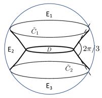
Suppose that , and is the union of two parallel circles contained in at distance from one another, with . Then, consists of the union of three connected components (here stand for up, lateral, and down, respectively). If is suitably small, then there are two smooth minimal catenoidal surfaces and , one stable and the other unstable, satisfying . Nonetheless if the initial partition satisfies ( ‣ 7.4), then, as a consequence of Proposition 7.4, both and are not admissible limits of Brakke flow as in Corollary 2.4, since there exists a smooth and homotopically non-trivial embedding having empty intersection with each of them. For instances, if and the initial partition is such that , , and , then the corresponding Brakke flows will converge, instead, to a singular minimal surface in consisting of the union , where are pieces of catenoids, and is a disc contained in the plane , which join together forming angles along the “free boundary” circle ; see Figure 1.
We will conclude the section with three remarks containing some interesting possible future research directions.
Remark 7.6.
First, we stress that the requirements on are rather flexible, above all in terms of regularity. It would be interesting to characterize, for a given strictly convex domain , all its admissible boundaries, namely all subsets such that there are and , as in Assumption 1.1 such that . A first observation is that admissible boundaries do not need to be countably -rectifiable, or to have finite -dimensional Hausdorff measure: for example, it is not difficult to construct an admissible in with , essentially a “fat” Cantor set in . The assumption requires any admissible boundary to have empty interior. It is unclear whether this condition is also sufficient for a subset to be admissible.
Remark 7.7.
Let us explicitly observe that, even in the case when (or more precisely ) is stationary, it is false in general that for . In other words, the approximation scheme which produces the Brakke flow may move the initial datum even when the latter is stationary. A simple example is a set consisting of two line segments with a crossing, for which multiple non-trivial solutions (depending on the choice of the initial partition) are possible; see Figure 2. In fact, one can prove that such one-dimensional configuration cannot stay time-independent with respect to the Brakke flow constructed in the present paper: [21, Theorem 2.2], indeed, shows that one-dimensional Brakke flows obtained in the present paper and in [20] necessarily satisfy a specific angle condition at junctions for a.e. time, with the only admissible angles being , , or degrees. Thus, depending on the initial labeling of domains, one of the two evolutions depicted in Figure 2 has to occur instantly.
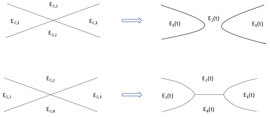
If is a smooth minimal surface with smooth boundary , the uniqueness theorem for classical MCF should allow as the unique solution, even if the latter is unstable (i.e. the second variation is negative for some direction). In other words, in the smooth case we expect that there is no other Brakke flow starting from other than the time-independent solution (notice, in passing, that both the area-reducing Lipschitz deformation step and the motion by smoothed mean curvature step in our time-discrete approximation of Brakke flow trivialize in this case - at least locally -, because smooth minimal surfaces are already locally area minimizing at suitably small scales around each point).
On the other hand, in [36] we show that time-dependent solutions may arise even from the existence, on , of singular points at which has a flat tangent cone, that is a tangent cone which is a plane with multiplicity . It would be interesting to characterize the regularity properties of those stationary with satisfying Assumption 1.1 and which do not allow any non-trivial Brakke flows (dynamically stable stationary varifolds, in the terminology introduced in [36]). We expect that such a should have some local measure minimizing properties.
Remark 7.8.
Let , and be as in Corollary 2.4 obtained as along a Brakke flow. Since is integral and stationary, for some -measurable function . One can check that and (after removing empty ’s if necessary) again satisfy the Assumption 1.1, thus we may apply Theorem 2.2 and obtain another Brakke flow with the same fixed boundary. Note that if we have , then may not be stationary, and the Brakke flow starting from non-stationary is genuinely time-dependent. We then obtain another stationary varifold as by Corollary 2.4. It is likely that, after a finite number of iterations, this process produces a unit density stationary varifold which does not move anymore. The other possibility is also interesting, in that we would have infinitely many different integral stationary varifolds with the same boundary condition, each having strictly smaller measure than the previous one.
References
- [1] William K. Allard. On the first variation of a varifold. Ann. of Math. (2), 95:417–491, (1972).
- [2] Kenneth A. Brakke. The motion of a surface by its mean curvature, volume 20 of Mathematical Notes. Princeton University Press, Princeton, N.J., 1978.
- [3] Kenneth A. Brakke. Soap films and covering spaces. J. Geom. Anal., 5(4):445–514, (1995).
- [4] Yun Gang Chen, Yoshikazu Giga, and Shun’ichi Goto. Uniqueness and existence of viscosity solutions of generalized mean curvature flow equations. J. Differential Geom., 33(3):749–786, (1991).
- [5] Guy David. Regularity of minimal and almost minimal sets and cones: J. Taylor’s theorem for beginners. In Analysis and geometry of metric measure spaces, volume 56 of CRM Proc. Lecture Notes, pages 67–117. Amer. Math. Soc., Providence, RI, (2013).
- [6] Guy David. Should we solve Plateau’s problem again? In Advances in analysis: the legacy of Elias M. Stein, volume 50 of Princeton Math. Ser., pages 108–145. Princeton Univ. Press, Princeton, NJ, (2014).
- [7] Camillo De Lellis, Francesco Ghiraldin, and Francesco Maggi. A direct approach to Plateau’s problem. J. Eur. Math. Soc. (JEMS), 19(8):2219–2240, (2017).
- [8] Camillo De Lellis, Jonas Hirsch, Andrea Marchese, and Salvatore Stuvard. Area-minimizing currents mod 2Q: linear regularity theory. Comm. Pure Appl. Math., (2020). https://doi.org/10.1002/cpa.21964.
- [9] Camillo De Lellis, Jonas Hirsch, Andrea Marchese, and Salvatore Stuvard. Regularity of area minimizing currents mod . Geom. Funct. Anal., 30(5):1224–1336, (2020).
- [10] Lawrence C. Evans and Joel Spruck. Motion of level sets by mean curvature. I. J. Differential Geom., 33(3):635–681, (1991).
- [11] Herbert Federer. Geometric measure theory. Die Grundlehren der mathematischen Wissenschaften, Band 153. Springer-Verlag New York Inc., New York, 1969.
- [12] Herbert Federer and Wendell H. Fleming. Normal and integral currents. Ann. of Math. (2), 72:458–520, (1960).
- [13] Jenny Harrison. Soap film solutions to Plateau’s problem. J. Geom. Anal., 24(1):271–297, (2014).
- [14] Jenny Harrison and Harrison Pugh. Existence and soap film regularity of solutions to Plateau’s problem. Adv. Calc. Var., 9(4):357–394, (2016).
- [15] Jenny Harrison and Harrison Pugh. Plateau’s problem. In Open problems in mathematics, pages 273–302. Springer, [Cham], (2016).
- [16] Gerhard Huisken. Nonparametric mean curvature evolution with boundary conditions. J. Differential Equations, 77(2):369–378, (1989).
- [17] Tom Ilmanen. Elliptic regularization and partial regularity for motion by mean curvature. Mem. Amer. Math. Soc., 108(520):x+90, (1994).
- [18] Tom Ilmanen, Peter Sternberg, and William P. Ziemer. Equilibrium solutions to generalized motion by mean curvature. J. Geom. Anal., 8(5):845–858, (1998). Dedicated to the memory of Fred Almgren.
- [19] Kota Kasai and Yoshihiro Tonegawa. A general regularity theory for weak mean curvature flow. Calc. Var. Partial Differential Equations, 50(1-2):1–68, (2014).
- [20] Lami Kim and Yoshihiro Tonegawa. On the mean curvature flow of grain boundaries. Ann. Inst. Fourier (Grenoble), 67(1):43–142, (2017).
- [21] Lami Kim and Yoshihiro Tonegawa. Existence and regularity theorems of one-dimensional Brakke flows. Interfaces Free Bound., 22:505–550, (2020).
- [22] Darren King, Francesco Maggi, and Salvatore Stuvard. Collapsing and the convex hull property in a soap film capillarity model. arXiv preprint arXiv:2002.06273, (2020).
- [23] Darren King, Francesco Maggi, and Salvatore Stuvard. Plateau’s problem as a singular limit of capillarity problems. Comm. Pure Appl. Math., (2020). https://doi.org/10.1002/cpa.21951.
- [24] Darren King, Francesco Maggi, and Salvatore Stuvard. Smoothness of collapsed regions in a capillarity model for soap films. arXiv preprint arXiv:2007.14868, (2020).
- [25] Gary M. Lieberman. The first initial-boundary value problem for quasilinear second order parabolic equations. Ann. Scuola Norm. Sup. Pisa Cl. Sci. (4), 13(3):347–387, (1986).
- [26] Francesco Maggi. Sets of finite perimeter and geometric variational problems, volume 135 of Cambridge Studies in Advanced Mathematics. Cambridge University Press, Cambridge, 2012.
- [27] Francesco Maggi, Antonello Scardicchio, and Salvatore Stuvard. Soap films with gravity and almost-minimal surfaces. Discrete Cont. Dyn. Syst., 39(12):6877–6912, (2019).
- [28] Annibale Magni, Carlo Mantegazza, and Matteo Novaga. Motion by curvature of planar networks, II. Ann. Sc. Norm. Super. Pisa Cl. Sci. (5), 15:117–144, (2016).
- [29] Carlo Mantegazza, Matteo Novaga, Alessandra Pluda, and Felix Schulze. Evolution of networks with multiple junctions. arXiv preprint arXiv:1611.08254, (2016).
- [30] Carlo Mantegazza, Matteo Novaga, and Vincenzo Maria Tortorelli. Motion by curvature of planar networks. Ann. Sc. Norm. Super. Pisa Cl. Sci. (5), 3(2):235–324, (2004).
- [31] Barbara Priwitzer. Mean curvature flow with Dirichlet boundary conditions in Riemannian manifolds with symmetries. Ann. Global Anal. Geom., 23(2):157–171, (2003).
- [32] Felix Schulze and Brian White. A local regularity theorem for mean curvature flow with triple edges. J. Reine Angew. Math., 758:281–305, (2020).
- [33] Leon Simon. Lectures on geometric measure theory, volume 3 of Proceedings of the Centre for Mathematical Analysis, Australian National University. Australian National University, Centre for Mathematical Analysis, Canberra, 1983.
- [34] Joel Spruck. Interior gradient estimates and existence theorems for constant mean curvature graphs in . Pure Appl. Math. Q., 3(3, Special Issue: In honor of Leon Simon. Part 2):785–800, (2007).
- [35] Peter Sternberg and William P. Ziemer. Generalized motion by curvature with a Dirichlet condition. J. Differential Equations, 114(2):580–600, (1994).
- [36] Salvatore Stuvard and Yoshihiro Tonegawa. Dynamical instability of minimal surfaces at flat singular points. arXiv preprint arXiv:2008.13728, (2020).
- [37] Yoshihiro Tonegawa. A second derivative Hölder estimate for weak mean curvature flow. Adv. Calc. Var., 7(1):91–138, (2014).
- [38] Yoshihiro Tonegawa. Brakke’s mean curvature flow: An introduction. SpringerBriefs in Mathematics. Springer, Singapore, 2019.
- [39] Brian White. Mean curvature flow with boundary. arXiv preprint arXiv:1901.03008, (2019).