An EPTAS for Budgeted Matroid Independent Set

We consider the budgeted matroid independent set (BMI) problem, defined as follows. We are given a set of elements $E$, a membership oracle for a collection of independent sets ${\mathcal{I}}\subseteq 2^{E}$, where $(E,{\mathcal{I}})$ is a matroid, a budget $\beta>0$, a cost function $c:E\to[0,\beta]$, and a profit function $p:E\rightarrow\mathbb{R}_{+}$. A solution for the problem is an independent set $X\in{\mathcal{I}}$ of total cost at most $\beta$ (i.e., $c(X)=\sum_{e\in X}c(e)\leq\beta$). The profit of a solution $X$ is $p(X)=\sum_{e\in X}p(e)$, and the objective is to find a solution of maximal profit.

BMI is a generalization of the classic $0/1$-knapsack problem, which is NP-hard and therefore unlikely to admit an exact polynomial-time algorithm. Thus, there is a long line of work on finding efficient approximations for knapsack and its variants (for comprehensive surveys see, e.g., [20, 17]).

Let $\textnormal{OPT}(I)$ be the value of an optimal solution for an instance $I$ of a maximization problem $\Pi$. For $\alpha\in(0,1]$, we say that ${\mathcal{A}}$ is an $\alpha$-approximation algorithm for $\Pi$ if, for any instance $I$ of $\Pi$, ${\mathcal{A}}$ outputs a solution of value at least $\alpha\textnormal{OPT}(I)$. A polynomial-time approximation scheme (PTAS) for a maximization problem $\Pi$ is a family of algorithms $({\mathcal{A}}_{{\varepsilon}})_{{\varepsilon}>0}$ such that, for any ${\varepsilon}>0$, ${\mathcal{A}}_{{\varepsilon}}$ is a polynomial-time $(1-{\varepsilon})$-approximation algorithm for $\Pi$; $({\mathcal{A}}_{{\varepsilon}})_{{\varepsilon}>0}$ is an EPTAS if the running time of ${\mathcal{A}}_{{\varepsilon}}$ is of the form $f\left(\frac{1}{{\varepsilon}}\right)\cdot n^{O(1)}$, where $f$ is an arbitrary function, and $n$ is the bit-length encoding size of the input instance; $({\mathcal{A}}_{{\varepsilon}})_{{\varepsilon}>0}$ is an FPTAS if the running time of ${\mathcal{A}}_{{\varepsilon}}$ is of the form $\left(\frac{n}{{\varepsilon}}\right)^{O(1)}$.

Polynomial-time approximation schemes allow us to obtain almost optimal solutions for NP-hard optimization problems via a speed-accuracy trade-off. However, the strong dependency of run-times on the error parameter, ${\varepsilon}>0$, often renders these schemes highly impractical. Thus, a natural goal is to seek the fastest scheme for a given problem, assuming one exists. Having obtained a PTAS, the next step is to consider possible improvements to an EPTAS, or even to an FPTAS. This is the focus of our work.

For the classic knapsack problem, a very efficient FPTAS exists since the 1970’s. Lawler’s scheme [19], based on ideas from [12], achieves a running time of $O(n\log 1/{\varepsilon}+1/{\varepsilon}^{4})$ for a $(1-{\varepsilon})$-approximation. In contrast, already the two-dimensional knapsack problem has a PTAS but does not admit an EPTAS [18]. For the well known multiple knapsack problem, Chekuri and Khanna [3] derived the first PTAS, which was later improved by Jansen to an EPTAS [13, 14]. The existence of an FPTAS is ruled out by a simple reduction from Partition [3]. More generally, resolving the complexity status of NP-hard optimization problem with respect to approximation schemes has been the focus of much research relating to resource allocation and scheduling (see, e.g., [24, 6, 8, 15, 16] and the surveys  [22, 23]).

For BMI, FPTASs are known for instances in which the matroid belongs to a restricted family. One notable example is multiple choice knapsack [19], where the elements are partitioned into groups, and a set is independent if it contains at most one element from each group. Another example is $1.5$-dimensional knapsack [2], in which a set is independent if it contains at most $k$ elements for some $k\geq 1$ (i.e., a uniform matroid constraint).

There are known results also for generalizations of BMI which involve multiple budget constraints or an additional matroid constraint. Specifically, Grandoni and Zenklusen developed in [9] a PTAS for multi-budgeted matroid independent set (MBMI), a generalization of BMI in which the costs are $d$-dimensional (for some constant $d\in\mathbb{N}$). The PTAS of [9] is based on integrality properties of a linear programming relaxation of the problem. As MBMI generalizes the two-dimensional knapsack problem, it does not admit an EPTAS unless $\textnormal{W}[1]=\textnormal{FPT}$ [18].

The budgeted matroid intersection problem is a generalization of BMI in which the input includes membership oracles for independent sets of two different matroids, and the solution must be an independent set of both matroids. A PTAS for budgeted matroid intersection was developed in [1]. The algorithm of [1] uses a Lagrangian relaxation along with some combinatorial properties of the problem to patch two solutions (i.e., a feasible solution with sub-optimal profit, and a non-feasible solution with high profit) into the final solution. The existence of an EPTAS (or an FPTAS) for budgeted matroid intersection is still open.

The multi-budgeted matroid intersection problem is a generalization of both multi-budgeted matroid independent set and budgeted matroid intersection, in which the cost function is $d$-dimensional, and the input contains two matroids. In [4] the authors developed a PTAS for multi-budgeted matroid intersection, based on randomized rounding of a solution for a linear programming (LP) relaxation of the problem.

The budgeted matroid independent set problem is also a special case of multiple knapsack with a matroid, a variant of BMI in which the input contains $m$ budgets $\beta_{1},\ldots,\beta_{m}$. A solution consists of $m$ sets $S_{1},\ldots,S_{m}$, where the cost of the $j$th set is at most the $j$th budget ($c(S_{j})\leq\beta_{j}$), and the union of the sets is an independent set of the matroid. A PTAS for the problem (based on randomized rounding) was given in [7]. The existence of an FPTAS is ruled out, as multiple knapsack is a special case [3].

To the best of our knowledge, BMI is studied here for the first time. A PTAS for the problem follows from known results for any of the above generalizations. In all cases, the running time of the scheme is dominated by an enumeration phase which guesses the most profitable elements in an optimal solution.

Our main result is an EPTAS for BMI, thus substantially improving the running times of existing schemes for the problem. Let ${\mathcal{K}}=(E,{\mathcal{I}},c,p,\beta)$ denote a BMI instance, $\textnormal{OPT}({\mathcal{K}})$ the profit of an optimal solution for ${\mathcal{K}}$, and $|{\mathcal{K}}|$ the bit-length encoding of the instance ${\mathcal{K}}$.

The improved running time of our algorithm is obtained by reducing the time complexity of the enumeration phase. Consider a BMI instance ${\mathcal{K}}=(E,{\mathcal{I}},c,p,\beta)$. Given some $0<{\varepsilon}<\frac{1}{2}$, we say that an element $e\in E$ is profitable if $p(e)>{\varepsilon}\cdot\textnormal{OPT}({\mathcal{K}})$. Our algorithm identifies a representative set of elements $R\subseteq E$ satisfying $|R|\leq f\left(\frac{1}{{\varepsilon}}\right)$, for a computable function $f$. Furthermore, we show that the BMI instance has a solution $S$ where all elements in $S\setminus R$ are non-profitable and $p(S)\geq(1-O({\varepsilon}))\cdot\textnormal{OPT}({\mathcal{K}})$. Thus, we can use enumeration to guess $S\cap R$ and then extend the solution using an LP relaxation similar to [9]. Crucial to our construction of $S$ is the notion of profit gap, used for identifying elements that may be added to $S$ by solving the LP (see Section 3). Since all the elements in $S\setminus R$ are non-profitable, the profit loss caused by the few non-integral entries is negligible. Moreover, since $|R|\leq f\left(\frac{1}{{\varepsilon}}\right)$, guessing $S\cap R$ can be done in $2^{f\left(\frac{1}{{\varepsilon}}\right)}$ steps (in fact, we obtain a slightly better running time), eliminating the dependency of enumeration on the input size. The representative set is identified via matroid basis minimization, which can be solved by a simple greedy algorithm (see Section 3).

For simplicity of the notation, for any set $A$ and an element $e$, we use $A+e$ and $A-e$ to denote $A\cup\{e\}$ and $A\setminus\{e\}$, respectively. Also, for any $k\in\mathbb{R}$ let $[k]=\{1,2,\ldots,\left\lfloor k\right\rfloor\}$. Finally, for a function $f:A\rightarrow B$ and a subset of elements $C\subseteq A$, we define $f(C)=\sum_{e\in C}f(e)$.

In this section we present an EPTAS for BMI. Our scheme initially handles elements of high profits. This is done by finding a small representative set out of which the scheme selects the most profitable elements in the solution. More elements, of lower profits, are then added to the solution using a linear program. For the remainder of this section, fix a BMI instance ${\mathcal{K}}=(E,{\mathcal{I}},c,p,\beta)$ and a parameter $0<{\varepsilon}<\frac{1}{2}$. W.l.o.g., for all $e\in E$ we assume that $\{e\}\in{\mathcal{I}}$ (otherwise $e$ cannot belong to any solution for ${\mathcal{K}}$).

Let $H({\mathcal{K}},{\varepsilon})=\{\ell\in E~{}|~{}p(\ell)>{\varepsilon}\cdot\textnormal{OPT}({\mathcal{K}})\}$ be the set of profitable elements in ${\mathcal{K}}$, and $E\setminus H({\mathcal{K}},{\varepsilon})$ the set of non-profitable elements; when understood from the context, we simply use $H=H({\mathcal{K}},{\varepsilon})$. We can easily obtain a PTAS by enumerating over all subsets of at most ${\varepsilon}^{-1}$ profitable elements to find the profitable elements in the solution. However, such exhaustive search is done in time $\Omega\left(|{\mathcal{K}}|^{{\varepsilon}^{-1}}\right)$, which cannot lead to an EPTAS. Thus, we take a different approach.

A key observation is that efficient solution can be obtained without enumerating over all subsets of profitable elements. Instead, we limit our scheme to a smaller search space using the notions of replacements and representative sets. Let $S$ be an independent set having a bounded number of elements. A replacement of $S$ is a subset of elements which can replace the profitable elements in $S$, resulting with an independent set of lower cost and almost the same profit. A representative set $R$ is a subset of elements which contains a replacement within $R$ for any independent set with bounded number of elements. Definitions 3.1 and 3.2 give the formal properties of replacements and representative sets, respectively. Let $q({\varepsilon})={\varepsilon}^{-{\varepsilon}^{-1}}$, and recall that ${\mathcal{I}}_{\leq q({\varepsilon})}=\{A\in{\mathcal{I}}~{}|~{}|A|\leq q({\varepsilon})\}$ (the selection of value for $q({\varepsilon})$ becomes clear in the proof of Lemma 3.3).

In particular, observe that for any solution $S$ of ${\mathcal{K}}$ we have that $S\cap H$ is a replacement of $S$; also, $E$ is a representative set. In the next lemma we show that there exists an almost optimal solution in which all profitable elements belong to a given representative set. Hence, guessing the profitable elements only requires enumerating over subsets of a representative set.

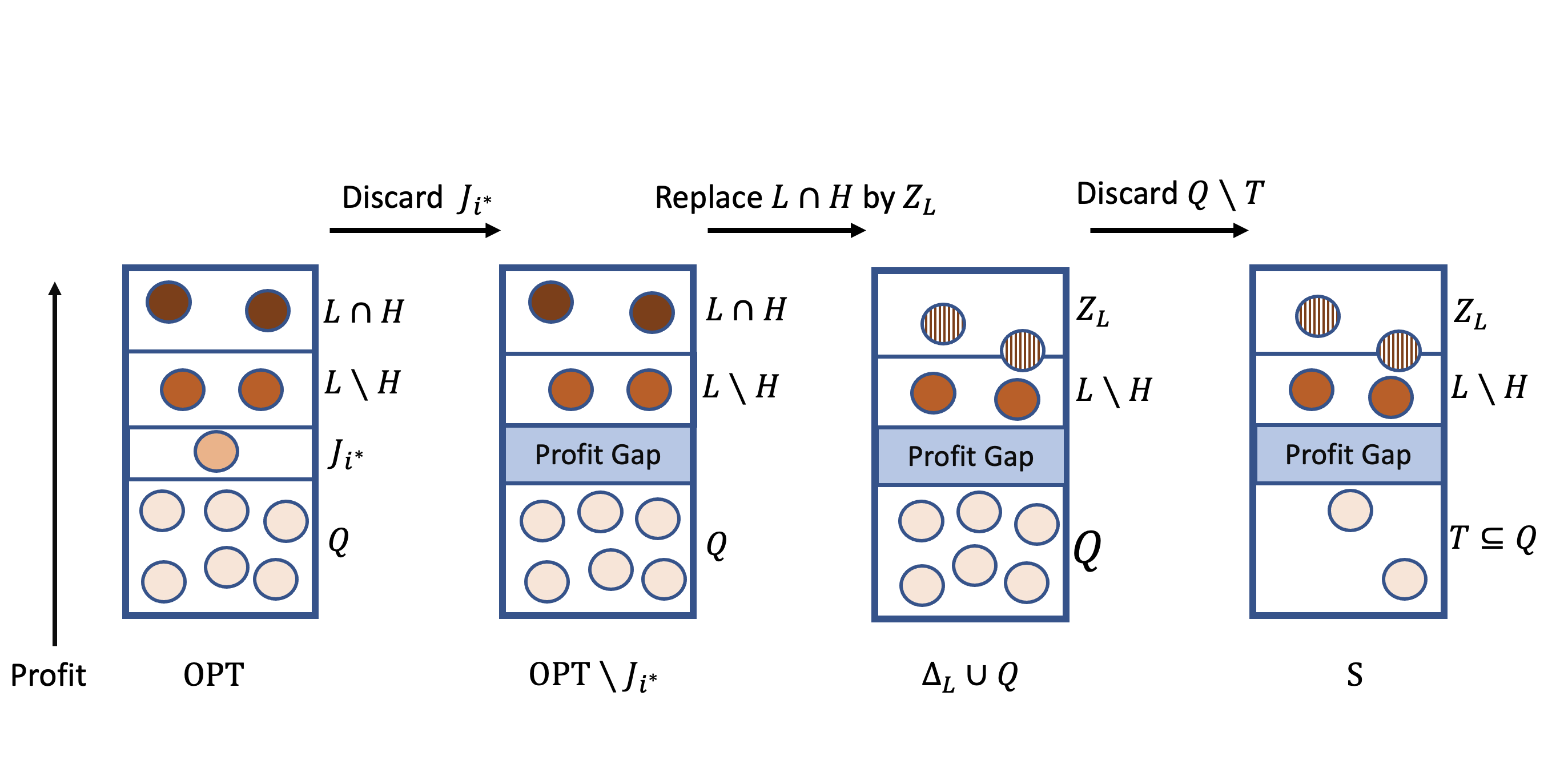
We give a brief outline of the proof of Lemma 3.3. Informally, we consider the elements in some optimal solution, OPT, in non-increasing order by profit. We then partition these elements into three sets: $L,J_{i^{*}}$ and $Q$, such that the maximal profit in $Q$ is at most ${\varepsilon}$ times the minimum profit in $L$. This is the profit gap of $L$ and $Q$. In addition, $L\in{\mathcal{I}}_{\leq q({\varepsilon})}$, and $p(J_{i^{*}})\leq{\varepsilon}\cdot\textnormal{OPT}({\mathcal{K}})$. Thus, we can use $Z_{L}\subseteq R$ as a replacement of $L$, i.e., $L\cap H$ will be replaced by elements in $Z_{L}$ (note that $Z_{L}$ is not necessarily a subset of the profitable elements). We now discard $J_{i^{*}}$, and define $\Delta_{L}=(L\setminus H)\cup Z_{L}$. As $\Delta_{L}\cup Q$ may not be an independent set, we use Observation 2.1 to construct $T\subseteq Q,|T|\geq|Q|-|L|$ such that $S=\Delta_{L}\cup T\in{\mathcal{I}}$. An illustration of the proof is given in Figure 1.

References

- [1] Berger, A., Bonifaci, V., Grandoni, F., Schäfer, G.: Budgeted matching and budgeted matroid intersection via the gasoline puzzle. Mathematical Programming 128(1), 355–372 (2011)
- [2] Caprara, A., Kellerer, H., Pferschy, U., Pisinger, D.: Approximation algorithms for knapsack problems with cardinality constraints. European Journal of Operational Research 123(2), 333–345 (2000)
- [3] Chekuri, C., Khanna, S.: A polynomial time approximation scheme for the multiple knapsack problem. SIAM Journal on Computing 35(3), 713–728 (2005)
- [4] Chekuri, C., Vondrák, J., Zenklusen, R.: Multi-budgeted matchings and matroid intersection via dependent rounding. In: Proceedings of the twenty-second annual ACM-SIAM symposium on Discrete Algorithms. pp. 1080–1097. SIAM (2011)
- [5] Cormen, T.H., Leiserson, C.E., Rivest, R.L., Stein, C.: Introduction to algorithms. MIT press (2022)
- [6] Das, S., Wiese, A.: On minimizing the makespan when some jobs cannot be assigned on the same machine. In: 25th Annual European Symposium on Algorithms, ESA. pp. 31:1–31:14 (2017)
- [7] Fairstein, Y., Kulik, A., Shachnai, H.: Modular and submodular optimization with multiple knapsack constraints via fractional grouping. In: 29th Annual European Symposium on Algorithms, ESA 2021, September 6-8, 2021, Lisbon, Portugal (Virtual Conference). pp. 41:1–41:16 (2021)
- [8] Grage, K., Jansen, K., Klein, K.M.: An EPTAS for machine scheduling with bag-constraints. In: The 31st ACM Symposium on Parallelism in Algorithms and Architectures. pp. 135–144 (2019)
- [9] Grandoni, F., Zenklusen, R.: Approximation schemes for multi-budgeted independence systems. In: European Symposium on Algorithms. pp. 536–548. Springer (2010)
- [10] Grötschel, M., Lovász, L., Schrijver, A.: Geometric algorithms and combinatorial optimization, vol. 2. Springer Science & Business Media (1993)
- [11] Heydrich, S., Wiese, A.: Faster approximation schemes for the two-dimensional knapsack problem. ACM Trans. Algorithms 15(4), 47:1–47:28 (2019)
- [12] Ibarra, O.H., Kim, C.E.: Fast approximation algorithms for the knapsack and sum of subset problems. Journal of the ACM (JACM) 22(4), 463–468 (1975)
- [13] Jansen, K.: Parameterized approximation scheme for the multiple knapsack problem. SIAM Journal on Computing 39(4), 1392–1412 (2010)
- [14] Jansen, K.: A fast approximation scheme for the multiple knapsack problem. In: SOFSEM 2012: Theory and Practice of Computer Science - 38th Conference on Current Trends in Theory and Practice of Computer Science, Špindlerův Mlýn, Czech Republic, January 21-27, 2012. Proceedings. pp. 313–324 (2012])
- [15] Jansen, K., Maack, M.: An EPTAS for scheduling on unrelated machines of few different types. Algorithmica 81(10), 4134–4164 (2019)
- [16] Jansen, K., Sinnen, O., Wang, H.: An EPTAS for scheduling fork-join graphs with communication delay. Theor. Comput. Sci. 861, 66–79 (2021)
- [17] Kellerer, H., Pferschy, U., Pisinger, D.: Knapsack problems. Springer (2004)
- [18] Kulik, A., Shachnai, H.: There is no EPTAS for two-dimensional knapsack. Information Processing Letters 110(16), 707–710 (2010)
- [19] Lawler, E.L.: Fast approximation algorithms for knapsack problems. Math. Oper. Res. 4(4), 339–356 (1979)
- [20] Pisinger, D., Toth, P.: Knapsack problems. In: Handbook of combinatorial optimization, pp. 299–428 (1998)
- [21] Schrijver, A.: Combinatorial optimization: polyhedra and efficiency, vol. 24. Springer (2003)
- [22] Schuurman, P., Woeginger, G.J.: Approximation schemes-a tutorial. Lectures on Scheduling (to appear) (2001)
- [23] Shachnai, H., Tamir, T.: Polynomial time approximation schemes. In: Handbook of Approximation Algorithms and Metaheuristics, Second Edition, Volume 1: Methologies and Traditional Applications, pp. 125–156 (2018)
- [24] Woeginger, G.J.: When does a dynamic programming formulation guarantee the existence of an FPTAS? In: Proceedings of the Tenth Annual ACM-SIAM Symposium on Discrete Algorithms, 17-19 January 1999, Baltimore, Maryland, USA. pp. 820–829 (1999)
Appendix A Solving the Linear Program
In this section we show how can be solved in polynomial time, thus proving Lemma 3.10.
The main idea is to show that the feasibility domain of is a well described polytope, and that a separation oracle for it can be implemented in polynomial time. Thus, using a known connection between separation and optimization, we obtain a polynomial-time algorithm which solves . Our initial goal, however, is to show that is indeed a linear program, for which we need a characterization of the matroid polytope via linear inequalities.
Let be a matroid. The matroid rank function of , , is defined by . That is, is the maximal size of an independent set which is also a subset of . The rank function is used in a characterization of a matroid polytope via a system of linear inequalities.
Theorem A.1 (Corollary 40.2b in [21]).
For any matroid , it holds that
Let be a BMI instance, and . By Theorem A.1 it holds that (6) is equivalent to the following linear program.