An End-to-End Framework for Marketing Effectiveness Optimization under Budget Constraint
Abstract.
Online platforms often incentivize consumers to improve user engagement and platform revenue. Since different consumers might respond differently to incentives, individual-level budget allocation is an essential task in marketing campaigns. Recent advances in this field often address the budget allocation problem using a two-stage paradigm: the first stage estimates the individual-level treatment effects using causal inference algorithms, and the second stage invokes integer programming techniques to find the optimal budget allocation solution. Since the objectives of these two stages might not be perfectly aligned, such a two-stage paradigm could hurt the overall marketing effectiveness.
In this paper, we propose a novel end-to-end framework to directly optimize the business goal under budget constraints. Our core idea is to construct a regularizer to represent the marketing goal and optimize it efficiently using gradient estimation techniques. As such, the obtained models can learn to maximize the marketing goal directly and precisely. We extensively evaluate our proposed method in both offline and online experiments, and experimental results demonstrate that our method outperforms current state-of-the-art methods. Our proposed method is currently deployed to allocate marketing budgets for hundreds of millions of users on a short video platform and achieves significant business goal improvements. Our code will be publicly available.
1. Introduction
Offering incentives (e.g., cash bonuses, discounts, coupons) to consumers are effective ways for online platforms to acquire new users, increase user engagement, and boost platform revenue (Lin et al., 2017; Zhao and Harinen, 2019; Zhao et al., 2019; Makhijani et al., 2019; Goldenberg et al., 2020; Zhang et al., 2021; Tu et al., 2021; Ai et al., 2022; Albert and Goldenberg, 2022; Zhou et al., 2023). For example, coupons in Taobao (Zhang et al., 2021) are offered to increase user activity, promotions in Booking (Goldenberg et al., 2020) can improve user satisfaction, cash bonuses in Kuaishou (Ai et al., 2022) are used to stimulate user retention, and promotions in Uber (Zhao and Harinen, 2019) can encourage users to start using a new product. Despite the effectiveness, these marketing campaigns could incur high costs, and thus the total budget is often capped in real-world scenarios. From the perspective of online platforms, the goal of a marketing campaign is often described as maximizing a specific business goal (e.g., user retention) under a specific budget constraint. To this end, allocating an appropriate amount of incentive to different users is essential for optimizing marketing effectiveness since different users could respond differently to incentives. This budget allocation problem has great practical implications and has been investigated for decades.
Many recent advances address the budget allocation problem using a two-stage paradigm (Zhao et al., 2019; Ai et al., 2022; Tu et al., 2021; Albert and Goldenberg, 2022): in the first stage the individual-level heterogeneous treatment effects are estimated using causal inference techniques, and then the estimated effects are fed into an integer programming formulation as coefficients to find the optimal allocation. However, the objectives of these two stages are fundamentally different, and in practice, we have observed these objectives are not perfectly aligned. For example, if the total budget is extremely low, then an effective allocation algorithm should distribute incentives only to a small subset of users who are fairly sensitive to incentives. In this case, an improved treatment effects predictor might have worse marketing effectiveness, if the model has a higher precision on all users on average but performs poorly on this small subset of users.
In this paper, we propose a novel end-to-end approach to optimize marketing effectiveness under budget constraints, directly and precisely. Our core idea is to construct a regularizer to represent the marketing goal, and further optimize it efficiently using gradient estimation techniques. Concretely, we use S-Learner (Künzel et al., 2019) based on Deep Neural Networks (DNNs) to predict the treatment effects of different users. Given the estimated treatment effects, we further formulate the budget allocation problem as a multiple choice knapsack problem (MCKP) (Kellerer et al., 2004), and exploit the Expected Outcome Metric method (EOM) to build an unbiased estimation (denoted as ) of the marketing goal (i.e., the expected business goal under a certain budget constraint). The function represents the marketing effectiveness and is the exact objective we want to maximize, thus we treat as a regularizer and integrate it into the training objective of the S-Learner model. However, there remains one challenge in doing so: since our construction process of involves solving a series of MCKPs using Lagrange multipliers and thus many non-differentiable operations are involved in, the automatic differentiation mechanism in modern machine learning libraries (such as TensorFlow (Abadi et al., 2015) and PyTorch (Paszke et al., 2019)) would not give correct gradients. Our solution to resolve this issue is to treat as a black-box function and exploit gradient estimation techniques such as the finite-difference method or natural evolution strategies (NES) (Wierstra et al., 2014) to obtain the gradients. As such, the regularizer could be effectively jointly optimized with the original learning objective of the S-Leanrer model. This regularizer endows the S-Learner model with an ability to directly learn from the marketing goal and further maximize it, in a principled way. Our proposed method is extensively evaluated on both offline simulations and online experiments. Experimental results demonstrate that our proposed end-to-end training framework can achieve significantly better marketing effectiveness, in comparison with current state-of-the-arts. We further deploy the proposed method in a large-scale short video platform to allocate cash bonuses to users to incentivize them to create more videos, and online A/B tests show our method significantly outperforms the baseline methods by at least 1.24% more video creators under the same budget, which is a tremendous improvement over these months. Currently, our proposed method is serving hundreds of millions of users.
2. Related Works
2.1. Budget Allocation
Starting from a common objective, many budget allocation methods have been proposed. Early methods (Guelman et al., 2015; Zhao et al., 2017; Zhao and Harinen, 2019) often select the amount of incentives for users heuristically after obtaining the heterogeneous treatment effects estimation. However, lacking an explicit optimization problem formulation could make these methods less effective in maximizing the marketing goal.
A popular way of allocating budget is to follow a two-stage paradigm (Zhao et al., 2019; Makhijani et al., 2019; Goldenberg et al., 2020; Tu et al., 2021; Ai et al., 2022; Albert and Goldenberg, 2022): in the first stage uplift models are used to predict the treatment effects, and in the second stage integer programming is invoked to find the optimal allocation. For instance, Zhao et al. (2019) propose to use a logit response model (Phillips, 2021) to predict treatment effects and then obtain the optimal allocation via root-finding for KKT conditions. Later, Tu et al. (2021) introduce various advanced estimators (including Causal Tree (Athey and Imbens, 2016), Causal Forest (Wager and Athey, 2018) and Meta-Learners (Sołtys et al., 2015; Künzel et al., 2019)) to estimate the heterogeneous effects. The second stage has also received much research attention. Makhijani et al. (2019) formulate the marketing goal as a Min-Cost Flow network optimization problem for better expressivity. More recently, Ai et al. (2022); Albert and Goldenberg (2022) use MCKP to represent the budget allocation problem in the discrete case and develop efficient solvers based on Lagrangian duality. Though effective, owing to the misalignment between the objectives of these two stages, solutions from these two-stage methods could be suboptimal.
Several methods have also been proposed to directly learn the optimal budget assignment policy (Xiao et al., 2019; Du et al., 2019; Goldenberg et al., 2020; Zou et al., 2020; Zhang et al., 2021; Zhou et al., 2023). Xiao et al. (2019); Zhang et al. (2021) develop reinforcement learning solutions based on constrained Markov decision process to directly learn an optimal policy. However, learning such complicated policies in a pure model-free black-box approach without exploiting the causal structures could suffer from sample inefficiency. Du et al. (2019); Zou et al. (2020); Goldenberg et al. (2020) propose to directly learn the ratios between values and costs in the binary treatment setting, and treatments could be first applied to users with higher scores. Later, a contemporary work (Zhou et al., 2023) proves the proposed loss in (Du et al., 2019; Zou et al., 2020) cannot achieve the correct rank when the loss converges. Furthermore, the method proposed in (Goldenberg et al., 2020) is applicable only if the budget constraint is that monetary ROI, which is not flexible enough for many marketing campaigns in online Internet platforms. Zhou et al. (2023) extend the decision-focused learning idea to the multiple-treatments setting and develop a loss function to learn decision factors for MCKP solutions. However, the proposed method relies on the assumption of diminishing marginal utility, which is often not strictly hold in practice.
2.2. Gradient Estimation
Estimating the gradients of a black-box function has been extensively studied for decades and widely used in the field of reinforcement learning (Sutton et al., 1999) and adversarial attack (Ilyas et al., 2018; Guo et al., 2019). The simplest approach is the finite-difference strategy, i.e., calculating the gradients by definition. The finite-difference strategy could give accurate gradients but might be computationally expensive if the independent variables of the black-box function have high dimensionalities. An alternative way of gradient estimation is natural evolution strategies (NES) (Wierstra et al., 2014), which generate several search directions to probe local geometrics of the black-box function and estimate the gradients based on sampled search directions. NES is generally more computationally efficient than the finite-difference strategy, but the estimated gradients are noisy. Antithetic sampling (Salimans et al., 2017) could be employed to reduce the variance of NES gradient estimation. In this paper, we present both finite-difference- and NES-based algorithms for gradient estimation.
3. Our End-to-End Framework
Many budget allocation methods follow a two-stage paradigm, which may lead to degraded performance due to the misalignment between the objectives of the two stages. We reckon it can be beneficial to properly incorporate the allocation process based on the second stage into the learning objective, such that the model can directly learn to maximize the marketing goal. In this section, we first introduce major notations, then briefly analyze the two-stage paradigm, finally we present our end-to-end training framework.
3.1. Notations
In most online Internet platforms, randomized controlled trials (RCT) could be easily deployed and thus a decent amount of RCT data could usually be collected at an acceptable cost in practice. As such, in this paper, we focus on training models using RCT data for simplicity and leave the exploration on exploiting observational data to future works. We use to denote the features for -th user in a certain user group. The term “user group” might refer to a group of RCT training users or a group of non-RCT users whose budgets are allocated by our model. The exact meaning of the term “user group” should be easily inferred from the context in this paper. We set mutually exclusive treatments, and each treatment represents a certain amount of incentives (e.g., cash bonus, or discount levels) assigned to the user. The treatment assigned to user in RCT is denoted by , and the user would have a binary response after receiving the treatment . The response shall be the business goal we want to maximize. Meanwhile, applying treatment to user would induce a non-negative cost . Each sample from an RCT dataset consists of a quadruple .
3.2. The Two-Stage Paradigm
As discussed, a lot of efforts have been devoted to two-stage budget allocation methods (Zhao et al., 2019; Makhijani et al., 2019; Goldenberg et al., 2020; Tu et al., 2021; Ai et al., 2022; Albert and Goldenberg, 2022). In this section, we briefly introduce common components in two-stage budget allocation methods. In the first stage, two-stage methods seek to build an uplift model to predict the uplifts of responses under all possible treatments. In principle, any uplift models could be applied in this stage, such as S-Learners (Künzel et al., 2019), R-Learners (Nie and Wager, 2021), Uplift Trees (Rzepakowski and Jaroszewicz, 2012), Causal Forests (Athey and Imbens, 2016), GRFs (Athey et al., 2019), ORFs (Oprescu et al., 2019) and LBCFs (Ai et al., 2022). Although some tree-based uplift models like GRFs (Athey et al., 2019) and ORFs (Oprescu et al., 2019) are unbiased uplift estimators with theoretical convergence guarantees, the splitting criteria in their tree-growing process are not flexible enough to be easily extended and integrated with our proposed regularizers. Thus in this paper, we restrict our attention to using S-Leaners with DNNs (Krizhevsky et al., 2012) as base models, just like (Zhou et al., 2023). A typical DNN S-Learner model would take the user feature as input and feed into a multi-layer perceptron (MLP) with several fully-connected layers to obtain the base hidden representation of the user , and then the model would branch headers (i.e., shadow MLPs) on the top of the base hidden representation to predict responses and costs for every possible treatment, where each treatment corresponds two headers (one header for response and the other header for cost). In general, any DNN architecture could be used in this stage provided the DNN model takes as input and outputs two -dimensional vectors for predicted responses/costs under all possible treatments, and in this paper, we use the simple architecture described above and leave the exploration on DNN architectures to future works. Let exhaustively collects learnable parameters of the above DNN S-Leaner , and let and denote the predicted responses/costs of . The predicted response and cost of applying treatment to user are denoted by and , respectively. Given a training set with RCT users, the DNN S-Learner is trained in the first stage by minimizing the following objective:
| (1) |
where is the cross entropy loss for the binary response, and is a suitable loss for the cost target. The formulation of could vary from one dataset to another. For example, on a dataset where the cost label is categorical, it could be reasonable to use a cross entropy-loss for , while on another dataset where the cost label is continuous, a regression loss would be more appropriate for . After minimizing the objective in Equation (1), given a feature vector of a user, the well-trained DNN S-Leaner model should predict unbiased estimations of expected responses/costs of this user under all possible treatments.
In the second stage, two-stage methods usually keep the uplift model fixed and use a multiple choice knapsack problem (MCKP) (Kellerer et al., 2004) formulation to maximize the marketing goal under the budget constraint. Suppose the total budget for a group of users is set to . The expected response of under treatment is denoted by , and could be predicted by the well-trained DNN S-Learner from the first stage: . Let denotes the expected cost of under treatment , and could also be similarily predicted by . Using the above coefficients and constants, two-stage methods typically construct the following MCKP to find the optimal personalized treatment assignment solution which could maximize the expected marketing goal under a given budget constraint:
| (2) | ||||
| s.t. | ||||
where the matrix represents the budget allocation solution for users. All entries in are either 0 or 1. Each row of has exactly one entry with value 1, and means user should be assigned with treatment . Although MCKP is proven to be NP-Hard (Kellerer et al., 2004), in practice we can approximately solve it by first making linear relaxation to get rid of the integer constraints and then converting it to the dual problem (Ai et al., 2022; Zhou et al., 2023). Specifically, the dual problem of MCKP has only one scalar variable under a constraint that (Kellerer et al., 2004), and the objective of dual problem is given by
| (3) |
The dual problem (3) could be efficiently solved via bisection methods such as Dyer-Zemel algorithm (Zemel, 1984) or dual gradient descent (Ai et al., 2022; Zhou et al., 2023). Once the optimal dual solution is obtained, the optimal solution of the primal MCKP (2) could be given by KKT conditions:
| (4) |
Interested readers can read the insightful paper (Kellerer et al., 2004) for more details about solving MCKPs.
3.3. Marketing Goal as a Regularizer
As discussed in Section 1, our core idea for end-to-end training is to construct a regularizer to represent the marketing goal (i.e., the expected response under a certain budget constraint) and optimize it efficiently using gradient estimation techniques. Suppose we have a batch of RCT users from the training set (we set the batch size to in all experiments), the S-Learner model could predict responses for each user and we shall stack their predicted responses into a matrix to simplify the notations, and the costs of applying arbitrary treatments to these users could also be stacked into a matrix in a similar way. In this section, we present our solution to design a function to map the predicted response matrix and cost matrix to the marketing goal and integrate into the training objective of the S-Leaner model as a regularizer.

EExample of sensitiveness curve between the empirical business goal (y-axis) and empirical cost (x-axis) in the marketing data
We use Expected Outcome Metric (EOM) method (Zhao et al., 2017; Ai et al., 2022; Zhou et al., 2023) to construct . Concretely, starting from any dual feasible solution , we can obtain the corresponding budget allocation solution via KKT conditions in Equation (4). Since is the Lagrangian multiplier associated with the budget constraint in the primal MCKP (2), we know from complementary slackness conditions that must be the primal optimal solution for another MCKP in which the total budget is set to be while other coefficients and remain unchanged. In other words, given any , the corresponding is the optimal budget allocation solution under a certain total budget constraint. Using the budget allocation solution , we can find the set of user indices (denoted by ) in the RCT users whose treatment on the RCT data is equal to the assigned treatment in :
| (5) |
where is the treatment applied to user in the RCT data. Based on the set , the per-capita response and per-capita cost could be empirically estimated by:
| (6) | ||||
where and denote the response and cost of user in the RCT data respectively, and represents the cardinality of set .
As discussed, the obtained is the optimal budget allocation solution for these users under a certain budget constraint, and thus we could tune the total budget by adjusting the value of dual feasible solution (Kellerer et al., 2004). As such, we could start from and gradually increase its value, and the total budget in MCKP would be accordingly decreased. In this process, we could plot empirical per-capita cost and empirical per-capita response in the same figure 111Note this curve might not be strictly monotonically increasing since the empirical estimation process is noisy. to illustrate the users’ expected responses under different costs, and an example figure is shown in Figure 1. Based on this curve, intuitively we can use bisection search to find a suitable such that the empirical per-capita cost equals the given per-capita budget in the original MCKP, and define as the empirical per-capita response at that : . All details of evaluating given and are summarized in Algorithm 1.
The bisection process in Algorithm 1 could also be extended to -ary search by adding more middle points in the search interval in each iteration. Although the bisection method and the -ary search method share the same asymptotic time complexity, in modern GPU devices the -ary search method could usually run faster if the implementation is properly vectorized.
Given a batch of training data with RCT users, instead of optimizing the original objective in Equation (1) for S-Learner, we could directly optimize the marketing effectiveness by minimizing the following regularized objective in this batch:
| (7) |
where is the original loss in Equation (1) on this batch, and is a scaling factor that balances the importance of the original objective and the regularizer .
If the gradient and could be obtained (see Section 3.4), we can integrate the gradient into the back-propagation process (see Section 3.5). As such, the regularizer could be jointly optimized with the original learning objective and the whole objective in Equation (7) could be efficiently solved in an end-to-end flavor. This endows the trained model with an ability to directly learn from the marketing goal and further maximize it, in a principled way.
3.4. Gradient Estimation
As shown in Algorithm 1, the construction of regularizer involves many non-differentiable operations. Thus if we naïvely implement Algorithm 1 as a computational graph in modern machine learning libraries such as TensorFlow (Abadi et al., 2015) and PyTorch (Paszke et al., 2019), the automatic differentiation mechanism would not generate correct gradients. In this section, we present our solution to overcome this challenge and calculate the (estimation of) gradient and . We treat as a black-box function, and use two strategies to estimate the gradients: 1) finite-difference strategy in Section 3.4.1, and 2) natural evolution strategies (NES) (Wierstra et al., 2014) in Section 3.4.2. For clarity of presentation, in this section, we would present the detailed solution for estimating only, and estimating for could be similarly performed.
3.4.1. Finite-Difference Strategy
Finite-difference strategy is commonly used in the field of black-box adversarial attack (Chen et al., 2017; Tu et al., 2019) to estimate the gradient of a complicated black-box function. Specifically, given predicted responses of a batch of RCT training users, the -th element in the gradient matrix could be estimated by:
| (8) |
where , is a small positive constant to perturb the input of the function, and is the standard basis matrix with only the -th component as 1. We use the symmetric difference quotient (Peter and Maria, 2014) to improve the numerical stability.
Using Equation (8), theoretically, we could estimate each entry of the matrix one by one, and finally stack results of all entries together to obtain the estimation of the entire gradient matrix , at the cost of evaluating the function times. However, the forward process of function is sophisticated, and thus evaluating the function for times could be computationally intensive in practice. To accelerate the finite-difference process, we use a strategy somewhat analogous to a coordinate descent: randomly masking some entries. Concretely, in each training iteration, instead of evaluating all entries of , we randomly select entries and evaluate these entries of using Equation (8) while other entries are set to zero. In practice, we could adjust the hyper-parameter to achieve a sensible trade-off between computational efficiency and the accuracy of the gradient estimation.
3.4.2. Natural Evolution Strategy
NES is a popular derivative-free numerical optimization algorithm and it is commonly used in the field of black-box adversarial attack (Ilyas et al., 2018, 2019; Guo et al., 2019). Suppose a random variable follows an isotropic normal distribution with as the center and as the covariance matrix: , where is a small positive constant and is a -by- identity matrix. NES seeks to maximize the expected value of function under the distribution of by estimating the gradient using the “log derivative trick”222Similar trick is also used in policy gradient algorithms in reinforcement learning.:
| (9) | ||||
where is the probability density function of the random variable . If the variance is small enough, the expected value of in Equation (9) should be close to , and thus we could use NES to estimate the gradient :
| (10) | ||||
where in the last equation we use empirical average value to estimate the expectation, is a sample from the standard normal distribution in the dimensional vector space, and is the number of sampling directions. Using Equation (10), we could obtain an unbiased estimation of the gradient in a derivative-free fashion. The hyper-parameter controls the trade-off between the computational efficiency and accuracy of NES.
Like other Monte Carlo methods, NES also suffers from high variance when estimating a vector in a high dimensional space. To reduce the variance, we employ antithetic sampling (Salimans et al., 2017) to generate sampling directions: we first sample i.i.d. Gaussian noises as , and then set the remaining directions by flipping the signs of previous directions: . This sampling strategy has been empirically verified to be effective in many previous works (Ilyas et al., 2018, 2019; Guo et al., 2019).
3.5. Training
In this section, we present our solution to train the DNN model to maximize the marketing goal, by optimizing the regularized objective in Equation (7). Common gradient descent based optimizers such as SGD or Adam (Kingma and Ba, 2015) would require the gradients w.r.t. DNN model parameter (i.e., ) to update , while in Section 3.4 we only have and . Thus, a back-propagation step which converts and to is required. To this end, we design the following surrogate loss :
| (11) |
where is a scaling factor that balances the importance of the original objective and the regularizer, is the matrix trace operator, and is the transpose of matrix and respectively, and is the operator to treat a certain variable as a constant and avoid back-propagation through it.333In TensorFlow this could be achieved via tf.stop_gradient(), and in PyTorch this could be achieved by tensor.detach(). Unlike the regularizer part of which is cumbersome to handle, the regularizer part of is a simple linear combination of elements in matrix and , which are output values from the last layer of the DNN model. As such, the gradient of w.r.t. could be easily obtained by running a standard back-propagation over the DNN model. Furthermore, it could be verified that and shares the same first order gradient: . Thus, with the help of the surrogate loss , we could effectively optimize the original regularized objective , and the well-trained DNN model shall learn to maximize the marketing goal in an end-to-end manner. Algorithm 2 summarizes all details for training.
4. Experimental Results
4.1. Datasets
We evaluate the efficacy of our method in three different datasets:
-
•
Synthetic dataset. To elaborate on key components of our idea (i.e., EOM and gradient estimation), we generate a synthetic dataset consisting of 10,000 RCT users. We set four different treatments (i.e., ), and the treatment applied to the -th user in RCT is randomly sampled from these four treatments with equal probabilities. We assume the -th user has a four-dimensional ground truth vector , where the -th element in (denoted by ) represents the probability of when treatment is applied to that user. We use the following three steps to generate : 1) the first element of (i.e., ) is sampled from the uniform distribution in , 2) to determine the remaining elements of , we sample three i.i.d. numbers from the uniform distribution in and sort these three numbers in descending order (denoted by ), and 2) these three numbers are used as incremental values of : let , where . Once the four-dimensional ground truth vector is generated, we get the -th element of the (denoted by ) and sample the binary response of the -th user from the Bernoulli distribution with probability . We assume the cost of applying the -th treatment to any user is . In other words, we set the -th element in ground-truth cost matrix to be , where . The synthetic dataset is designed for illustrating the effectiveness of EOM and gradient estimation, thus the features of users are omitted in this dataset.
-
•
CRITEO-UPLIFT v2 (Diemert et al., 2018). This publicly available dataset is designed for evaluating models for uplift modeling. This dataset contains 13.9 million samples which are collected from an RCT. Each sample has 12 dense features, one binary treatment indicator, and two binary labels: visit and conversion. In this dataset, treatment is defined as whether the user is targeted by advertising or not, and labels are defined as positive if the user visited/converted on the advertiser’s website during a test period of two weeks. To evaluate different budget allocation methods, we follow (Zhou et al., 2023) and use the visit/conversion label as the cost/value respectively. We compare the performance of our proposed method with state-of-the-arts in CRITEO-UPLIFT v2 to demonstrate the effectiveness of our method.
-
•
KUAISHOU-PRODUCE-COIN. Produce Coin is a common marketing campaign to incentivize short video creators to upload more short videos in Kuaishou. In this campaign, we provide a prized task to each short video creator on the Kuaishou platform. Concretely, in each task, if a creator uploads a video within 24 hours, he/she will receive a certain amount of coins as a reward. Each creator could see the number of coins he/she could possibly obtain, and if the number seems attractive enough the creator might finish the task to collect these coins. We manually select 30 distinct levels of coins (e.g., 1 coin, 2 coins, ), and each creator will be assigned one of these 30 levels. The amount of coins could be personalized to maximize the total amount of video uploads under the constraint that the total amount of coins does not exceed a certain limit. In this dataset, we define treatment as the level of coins, thus we have treatments. For the user (i.e., creator) , the response would be if the user has successfully completed the task, and otherwise, we set . The cost of applying a treatment to would be defined as the real number of coins sent to : if we set the cost to the number of coins corresponding to the assigned treatment, and if we set the cost to zero. To collect this dataset we conduct an RCT for one week. In this RCT, we randomly sample one reward level from predefined 30 levels with equal probabilities for each user as the treatment and collect the response/cost label from the logs. This dataset contains 82.4 million samples, and we deploy several models trained on this dataset in the Kuaishou platform to evaluate the online performance of different methods. To protect data privacy, we normalize the per-capita response/cost and report the normalized values on all tables and figures.
4.2. Evaluation Metrics
We use the following evaluation metrics to evaluate and compare the performance of different methods:
-
•
AUCC (Area Under the Cost Curve) in (Du et al., 2019). AUCC is commonly used in existing literatures (Du et al., 2019; Ai et al., 2022; Zhou et al., 2023) to evaluate the ranking performance of uplift models in the two-treatment setting. Interested readers can check the original paper (Du et al., 2019) for more details about the evaluation process of AUCC. In this paper, we use AUCC to compare the performance of different methods in CRITEO-UPLIFT v2.
-
•
EOM (Expected Outcome Metric). EOM or similar metric is also commonly used in existing literatures (Ai et al., 2022; Zhou et al., 2023) to empirically estimate the expected outcome (e.g., per-capita response or per-capita cost) for arbitrary budget allocation policy. EOM can make an unbiased estimation of any outcome, provided that outcome is calculable given a budget allocation solution on RCT data. Thus, EOM is more flexible than AUCC in practice. In this paper, we use EOM in the synthetic dataset and the KUAISHOU-PRODUCE-COIN dataset to evaluate different budget allocation methods, and technical details of EOM have been introduced in Equation (5) and Equation (6) in Section 3.3.
4.3. Implementation Details
Implementation details on different datasets are shown as follows:
-
•
The synthetic dataset. To illustrate the basic idea of EOM and gradient estimation in our proposed method, we first generate a cost matrix and a value matrix as the starting point, and then use the Adam optimizer with a learning rate 0.005 to optimize by maximizing for 100 gradient ascent steps. For the starting point of cost matrix , we directly use the ground-truth cost matrix and keep it fixed during gradient ascent. For the starting point of value matrix , we use the same procedure as described in Section 4.1 to re-generate a random matrix which satisfies the following conditions for all : 1) , and 2) . We set the per-capita budget to 2.0 for evaluating the function. Since features of users are omitted in the synthetic dataset, we could not expect any generalization. Thus, we treat all 10,000 samples as training samples and report per-capita response and per-capita cost estimated by EOM on all training samples.
-
•
CRITEO-UPLIFT v2. We compare our proposed method with the following baseline methods in terms of AUCC:
-
–
TSM-SL. The baseline two-stage method in many existing literatures (Ai et al., 2022; Zhao et al., 2019; Zhou et al., 2023). In the first stage, a DNN-based S-Learner model is exploited to predict the conversion uplifts and visit uplifts for individuals. In the second stage, an MCKP formulation could be used to find the optimal budget allocation solution. However for AUCC, the explicit budget allocation solution is not required, and we simply rank different individuals by the ratio between the conversion uplifts and visit uplifts and use the rank to compute AUCC.
- –
- –
Following (Zhou et al., 2023), we randomly sample 70% samples from the dataset as the training set, and the remaining samples are used as the test set. We report the performance of different methods in the test set, and for baseline methods, we directly cite results from (Zhou et al., 2023). For our proposed method, we use a DNN architecture described in Section 3.2: the base DNN is a 4-layer MLP (hidden sizes 512-256-128-64), and each header DNN is a 2-layer MLP (hidden sizes 32-1). We insert a ReLU activation layer after each fully connected layer in both base DNN and header DNN, except the final output layer in header DNN. We also insert a Batch Normalization layer (Ioffe and Szegedy, 2015) after the activation layer for faster convergence. The value of in the surrogate loss in Equation (11) is set to 200. For the finite-difference strategy, we set and . For NES, we set and . The MSRA initialization (He et al., 2015) is invoked to initialize all weight matrices in our model. The randomly initialized DNN S-Learner model is trained using the Adam optimizer with a learning rate of 0.0001 for 10 epochs. In each training step, the per-capita budget for evaluating the function is randomly sampled from a uniform distribution in . Following (Zhou et al., 2023), we run our proposed method 20 times and report the mean and variance of results.
-
–
-
•
KUAISHOU-PRODUCE-COIN. To demonstrate the effectiveness of our proposed training framework in real-world scenarios, we conduct both offline evaluation and online evaluation to compare our proposed method and TSM-SL. The offline experiment and online experiment share the following settings:
-
–
The architecture for base DNN header DNN is kept the same as in the CRITEO-UPLIFT v2 dataset.
-
–
We train the DNN S-Learner model using the Adam optimizer with a learning rate of 0.0003 for 20 epochs. To make a fair comparison, we use identical feature engineering/DNN architecture/training policies for our proposed method and TSM-SL.
-
–
In each training step, the per-capita budget for evaluating the function is randomly sampled from a uniform distribution in .
Furthermore, in the offline experiment:
-
–
We randomly sample 80% of users from the KUAISHOU-PRODUCE-COIN dataset as the training set and the remaining 20% is used as the test set.
-
–
We employ EOM and bisection to find the value of per-capita response when per-capita cost equals 1.2, and this metric is used to measure the performance of different methods.
In the online experiment:
-
–
All samples in the KUAISHOU-PRODUCE-COIN dataset are used for training and the obtained well-trained models are deployed in an online A/B test in the Kuaishou platform to compare the efficacy of their budget allocation policies in the real world.
-
–
The online A/B test is conducted for one week. There are 14.2 million users in the online A/B test, and these users are disjoint for users in the KUAISHOU-PRODUCE-COIN dataset. We randomly partition 14.2 million users into two equally sized groups, one group for our proposed method and the other group for TSM-SL. For each group, the reported per-capita response/cost is directly computed over the entire 7.1 million users, and EOM is not employed.
-
–


4.4. Results on Synthetic Dataset
Results on the synthetic dataset are summarized in Figure 2. The black line in Figure 2(a) shows the statistics about per-capita cost and per-capita value in RCT. As discussed in Section 3.3, starting from any cost and value matrix we could obtain a series of budget allocation solutions corresponding to different budgets, and further invoke EOM to empirically estimate the per-capita value and per-capita cost for each budget allocation solution. We perform the above EOM procedure using ground-truth and , and plot the trajectory of and as the red dotted line in Figure 2(a). The value of function for ground-truth and is .
To verify the effectiveness of the gradient estimation process, we first generate initial and as described in Section 4.3 and study the cosine similarity between our estimated gradient and the precise gradient. To this end, we first set and use the finite-difference strategy to calculate the precise gradient . Then, we use NES to estimate (Equation (10)) and gradually increase . Finally, we check the cosine similarity between the NES estimated gradient and the precise gradient. Figure 2(b) shows the relations between cosine similarity and , and we can see that as more sampling directions are involved in NES, the estimated gradients are more accurate.
We further plug the estimated gradient by NES into an Adam optimizer to maximize , which represents the per-capita value when the per-capita cost equals 2.0. Figure 2(c) shows the per-capita value and per-capita cost of initial and . The value of function for initial and is . After 100 gradient ascent steps, we can increase the value of function from 0.1996 to 0.2141. Figure 2(d) shows the per-capita value and per-capita cost of optimized and . By comparing Figure 2(c) and Figure 2(d), we see that our proposed method could effectively increase the value of function. From the properties of EOM, we know that would be an unbiased estimator of the marketing goal. As such, the marketing goal could be effectively maximized. Since we only have 10,000 data samples, the Adam optimizer could severely overfit the training data and thus in Figure 2(d) there might be a peak around the region where the per-capita budget equals 2.0.
4.5. Results on CRITEO-UPLIFT v2
| Method | AUCC |
|---|---|
| TSM-SL | 0.7561 0.0113 |
| Direct Rank (Du et al., 2019) | 0.7562 0.0131 |
| DRP (Zhou et al., 2023) | 0.7739 0.0002 |
| Ours-NES | 0.7849 0.0167 |
| Ours-FD | 0.7904 0.0096 |
Results on CRITEO-UPLIFT v2 are summarized in Table 1. Ours-FD and Ours-NES refer to our proposed method with finite-difference strategy / NES as the gradient estimator, respectively. We see both Ours-FD and Ours-NES significantly outperform all competitive methods in the sense of AUCC. Ours-FD has the highest variance in AUCC for 20 runs, and this phenomenon could be partially explained by the fact that NES gradients are noisy. Although the performance of Ours-FD surpasses that of Ours-NES, Ours-FD costs 4x more running times on an NVIDIA Tesla T4 GPU (Ours-FD 17.6 hours v.s. Ours-NES 4.3 hours) since we need to evaluate the function for more times.
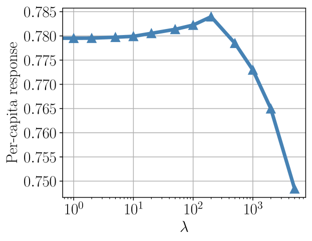
4.6. Results on KUAISHOU-PRODUCE-COIN
We adopt Ours-FD for the KUAISHOU-PRODUCE-COIN dataset and compare it with TSM-SL.
Offline performance on KUAISHOU-PRODUCE-COIN
4.6.1. Offline Evaluation
We are interested in how the value of in Equation (11) affects the performance of Ours-FD. We set and measure the performance of Ours-FD. For each value of , we train the model four times and report their average performance. Figure 3 illustrates the impact of in Equation (11) in Ours-FD. By definition, we know that if we set , Ours-FD would be reduced to TSM-SL. If , the regularizer would take effect and the DNN S-Learner model could learn from the marketing goal directly. However, if is too large, the regularizer could dominate the training objective and the predicted responses and costs could be far away from their ground-truth values thus the training process could be unstable. In Figure 3, when the per-capita response would increase with , and it is clear that our regularizer is beneficial for the marketing goal in this region. Furthermore, if , the performance of Ours-FD would be worse than that of TSM-SL since the training process becomes unstable.
4.6.2. Online Evaluation
For online evaluation, we re-train the model using the entire KUAISHOU-PRODUCE-COIN dataset. We deploy Ours-FD with and TSM-SL into the online A/B test. To measure the performance of different methods, we calculate the per-capita response and per-capita cost by averaging the results over seven days. When compared with TSM-SL, Ours-FD achieves a -0.369% lower per-capita cost and a 1.24% higher per-capita response simultaneously, which is considered to be a significant improvement over these months. The Ours-FD model is currently deployed to allocate marketing budgets for hundreds of millions of users.
5. Conclusion
In this paper, we investigate the end-to-end training framework in the budget allocation problem. We formulate the business goal under a certain budget constraint as a black-box regularizer and develop two efficient gradient estimation algorithms to optimize it. For both gradient estimation algorithms, we suggest a hyper-parameter to trade off the computation complexity and the accuracy of estimated gradients. Our proposed method shall endow the well-trained DNN model with the ability to directly learn from the marketing goal and further maximize it. Extensive experiments on three datasets have shown the superiority of our method in both offline simulation and online experiments. Our future work will focus on reducing the variance for gradient estimation and applying this approach in more complicated real-world marketing scenarios.
References
- (1)
- Abadi et al. (2015) Martín Abadi, Ashish Agarwal, Paul Barham, Eugene Brevdo, Zhifeng Chen, Craig Citro, Greg S. Corrado, Andy Davis, Jeffrey Dean, Matthieu Devin, Sanjay Ghemawat, Ian Goodfellow, Andrew Harp, Geoffrey Irving, Michael Isard, Yangqing Jia, Rafal Jozefowicz, Lukasz Kaiser, Manjunath Kudlur, Josh Levenberg, Dandelion Mané, Rajat Monga, Sherry Moore, Derek Murray, Chris Olah, Mike Schuster, Jonathon Shlens, Benoit Steiner, Ilya Sutskever, Kunal Talwar, Paul Tucker, Vincent Vanhoucke, Vijay Vasudevan, Fernanda Viégas, Oriol Vinyals, Pete Warden, Martin Wattenberg, Martin Wicke, Yuan Yu, and Xiaoqiang Zheng. 2015. TensorFlow: Large-Scale Machine Learning on Heterogeneous Systems. https://www.tensorflow.org/ Software available from tensorflow.org.
- Ai et al. (2022) Meng Ai, Biao Li, Heyang Gong, Qingwei Yu, Shengjie Xue, Yuan Zhang, Yunzhou Zhang, and Peng Jiang. 2022. LBCF: A Large-Scale Budget-Constrained Causal Forest Algorithm. In WWW 2022. 2310–2319.
- Albert and Goldenberg (2022) Javier Albert and Dmitri Goldenberg. 2022. E-Commerce Promotions Personalization via Online Multiple-Choice Knapsack with Uplift Modeling. In CIKM 2022. 2863–2872.
- Athey and Imbens (2016) Susan Athey and Guido Imbens. 2016. Recursive partitioning for heterogeneous causal effects. Proceedings of the National Academy of Sciences 113, 27 (2016), 7353–7360.
- Athey et al. (2019) Susan Athey, Julie Tibshirani, and Stefan Wager. 2019. Generalized random forests. The Annals of Statistics 47, 2 (2019), 1148–1178.
- Chen et al. (2017) Pin-Yu Chen, Huan Zhang, Yash Sharma, Jinfeng Yi, and Cho-Jui Hsieh. 2017. Zoo: Zeroth order optimization based black-box attacks to deep neural networks without training substitute models. In Proceedings of the 10th ACM workshop on artificial intelligence and security. 15–26.
- Diemert et al. (2018) Eustache Diemert, Artem Betlei, Christophe Renaudin, and Massih-Reza Amini. 2018. A large scale benchmark for uplift modeling. In SIGKDD 2018.
- Du et al. (2019) Shuyang Du, James Lee, and Farzin Ghaffarizadeh. 2019. Improve User Retention with Causal Learning. In SIGKDD Workshop on Causal Discovery 2019. PMLR, 34–49.
- Goldenberg et al. (2020) Dmitri Goldenberg, Javier Albert, Lucas Bernardi, and Pablo Estevez. 2020. Free lunch! retrospective uplift modeling for dynamic promotions recommendation within roi constraints. In ACM Conference on Recommender Systems 2020. 486–491.
- Guelman et al. (2015) Leo Guelman, Montserrat Guillén, and Ana M Pérez-Marín. 2015. Uplift random forests. Cybernetics and Systems 46, 3-4 (2015), 230–248.
- Guo et al. (2019) Yiwen Guo, Ziang Yan, and Changshui Zhang. 2019. Subspace attack: Exploiting promising subspaces for query-efficient black-box attacks. NeurIPS 2019 32.
- He et al. (2015) Kaiming He, Xiangyu Zhang, Shaoqing Ren, and Jian Sun. 2015. Delving deep into rectifiers: Surpassing human-level performance on imagenet classification. In ICCV 2015. 1026–1034.
- Ilyas et al. (2018) Andrew Ilyas, Logan Engstrom, Anish Athalye, and Jessy Lin. 2018. Black-box adversarial attacks with limited queries and information. In ICML 2018. PMLR, 2137–2146.
- Ilyas et al. (2019) Andrew Ilyas, Logan Engstrom, and Aleksander Madry. 2019. Prior Convictions: Black-box Adversarial Attacks with Bandits and Priors. In ICLR 2019.
- Ioffe and Szegedy (2015) Sergey Ioffe and Christian Szegedy. 2015. Batch normalization: Accelerating deep network training by reducing internal covariate shift. In ICML 2015. pmlr, 448–456.
- Kellerer et al. (2004) Hans Kellerer, Ulrich Pferschy, and David Pisinger. 2004. The multiple-choice knapsack problem. In Knapsack Problems. Springer, 317–347.
- Kingma and Ba (2015) Diederik P Kingma and Jimmy Ba. 2015. Adam: A Method for Stochastic Optimization. In ICLR 2015.
- Krizhevsky et al. (2012) Alex Krizhevsky, Ilya Sutskever, and Geoffrey E Hinton. 2012. Imagenet classification with deep convolutional networks. In NIPS 2012, Vol. 1097.
- Künzel et al. (2019) Sören R Künzel, Jasjeet S Sekhon, Peter J Bickel, and Bin Yu. 2019. Metalearners for estimating heterogeneous treatment effects using machine learning. Proceedings of the national academy of sciences 116, 10 (2019), 4156–4165.
- Lin et al. (2017) Ying-Chun Lin, Chi-Hsuan Huang, Chu-Cheng Hsieh, Yu-Chen Shu, and Kun-Ta Chuang. 2017. Monetary discount strategies for real-time promotion campaign. In WWW 2017. 1123–1132.
- Makhijani et al. (2019) Rahul Makhijani, Shreya Chakrabarti, Dale Struble, and Yi Liu. 2019. LORE: a large-scale offer recommendation engine with eligibility and capacity constraints. In ACM Conference on Recommender Systems 2019. 160–168.
- Nie and Wager (2021) Xinkun Nie and Stefan Wager. 2021. Quasi-oracle estimation of heterogeneous treatment effects. Biometrika 108, 2 (2021), 299–319.
- Oprescu et al. (2019) Miruna Oprescu, Vasilis Syrgkanis, and Zhiwei Steven Wu. 2019. Orthogonal random forest for causal inference. In ICML 2019. PMLR, 4932–4941.
- Paszke et al. (2019) Adam Paszke, Sam Gross, Francisco Massa, Adam Lerer, James Bradbury, Gregory Chanan, Trevor Killeen, Zeming Lin, Natalia Gimelshein, Luca Antiga, et al. 2019. Pytorch: An imperative style, high-performance deep learning library. In NeurIPS 2019, Vol. 32.
- Peter and Maria (2014) D Lax Peter and Shea Terrell Maria. 2014. Calculus With Applications.
- Phillips (2021) Robert L Phillips. 2021. Pricing and revenue optimization. In Pricing and Revenue Optimization. Stanford university press.
- Rzepakowski and Jaroszewicz (2012) Piotr Rzepakowski and Szymon Jaroszewicz. 2012. Decision trees for uplift modeling with single and multiple treatments. Knowledge and Information Systems 32, 2 (2012), 303–327.
- Salimans et al. (2017) Tim Salimans, Jonathan Ho, Xi Chen, Szymon Sidor, and Ilya Sutskever. 2017. Evolution strategies as a scalable alternative to reinforcement learning. arXiv preprint arXiv:1703.03864 (2017).
- Sołtys et al. (2015) Michał Sołtys, Szymon Jaroszewicz, and Piotr Rzepakowski. 2015. Ensemble methods for uplift modeling. Data Mining and Knowledge Discovery 6, 29 (2015), 1531–1559.
- Sutton et al. (1999) Richard S Sutton, David McAllester, Satinder Singh, and Yishay Mansour. 1999. Policy gradient methods for reinforcement learning with function approximation. NeurIPS 1999 12 (1999).
- Tu et al. (2019) Chun-Chen Tu, Paishun Ting, Pin-Yu Chen, Sijia Liu, Huan Zhang, Jinfeng Yi, Cho-Jui Hsieh, and Shin-Ming Cheng. 2019. Autozoom: Autoencoder-based zeroth order optimization method for attacking black-box neural networks. In AAAI 2019, Vol. 33. 742–749.
- Tu et al. (2021) Ye Tu, Kinjal Basu, Cyrus DiCiccio, Romil Bansal, Preetam Nandy, Padmini Jaikumar, and Shaunak Chatterjee. 2021. Personalized treatment selection using causal heterogeneity. In WWW 2021. 1574–1585.
- Wager and Athey (2018) Stefan Wager and Susan Athey. 2018. Estimation and inference of heterogeneous treatment effects using random forests. J. Amer. Statist. Assoc. 113, 523 (2018), 1228–1242.
- Wierstra et al. (2014) Daan Wierstra, Tom Schaul, Tobias Glasmachers, Yi Sun, Jan Peters, and Jürgen Schmidhuber. 2014. Natural evolution strategies. JMLR 2014 15, 1 (2014), 949–980.
- Xiao et al. (2019) Shuai Xiao, Le Guo, Zaifan Jiang, Lei Lv, Yuanbo Chen, Jun Zhu, and Shuang Yang. 2019. Model-based constrained MDP for budget allocation in sequential incentive marketing. In CIKM 2019. 971–980.
- Zemel (1984) Eitan Zemel. 1984. An O (n) algorithm for the linear multiple choice knapsack problem and related problems. Information processing letters 18, 3 (1984), 123–128.
- Zhang et al. (2021) Yang Zhang, Bo Tang, Qingyu Yang, Dou An, Hongyin Tang, Chenyang Xi, Xueying Li, and Feiyu Xiong. 2021. BCORLE (): An Offline Reinforcement Learning and Evaluation Framework for Coupons Allocation in E-commerce Market. In NeurIPS 2021, Vol. 34. 20410–20422.
- Zhao et al. (2019) Kui Zhao, Junhao Hua, Ling Yan, Qi Zhang, Huan Xu, and Cheng Yang. 2019. A Unified Framework for Marketing Budget Allocation. In SIGKDD 2019. 1820–1830.
- Zhao et al. (2017) Yan Zhao, Xiao Fang, and David Simchi-Levi. 2017. Uplift modeling with multiple treatments and general response types. In SIAM 2017. SIAM, 588–596.
- Zhao and Harinen (2019) Zhenyu Zhao and Totte Harinen. 2019. Uplift modeling for multiple treatments with cost optimization. In IEEE International Conference on Data Science and Advanced Analytics (DSAA) 2019. IEEE, 422–431.
- Zhou et al. (2023) Hao Zhou, Shaoming Li, Guibin Jiang, Jiaqi Zheng, and Dong Wang. 2023. Direct Heterogeneous Causal Learning for Resource Allocation Problems in Marketing. In AAAI 2023.
- Zou et al. (2020) Will Y Zou, Shuyang Du, James Lee, and Jan Pedersen. 2020. Heterogeneous causal learning for effectiveness optimization in user marketing. arXiv preprint arXiv:2004.09702 (2020).