This paper was converted on www.awesomepapers.org from LaTeX by an anonymous user.
Want to know more? Visit the Converter page.

An encounter-based approach for restricted diffusion with a gradient drift

Denis S. Grebenkov [email protected] 1 Laboratoire de Physique de la Matière Condensée (UMR 7643),
CNRS – Ecole Polytechnique, IP Paris, 91120 Palaiseau, France
2 Institute for Physics and Astronomy, University of Potsdam, 14476 Potsdam-Golm, Germany
Abstract

We develop an encounter-based approach for describing restricted diffusion with a gradient drift towards a partially reactive boundary. For this purpose, we introduce an extension of the Dirichlet-to-Neumann operator and use its eigenbasis to derive a spectral decomposition for the full propagator, i.e., the joint probability density function for the particle position and its boundary local time. This is the central quantity that determines various characteristics of diffusion-influenced reactions such as conventional propagators, survival probability, first-passage time distribution, boundary local time distribution, and reaction rate. As an illustration, we investigate the impact of a constant drift onto the boundary local time for restricted diffusion on an interval. More generally, this approach accesses how external forces may influence the statistics of encounters of a diffusing particle with the reactive boundary.

pacs:
02.50.-r, 05.40.-a, 02.70.Rr, 05.10.Gg
: J. Phys. A: Math. Gen.

Keywords: Boundary local time; Reflected Brownian motion; Diffusion-influenced reactions; Surface reactivity; Robin boundary condition; Heterogeneous catalysis

1 Introduction

Many transport processes in nature and industry are described by an overdamped Langevin equation for the random position 𝑿t\bm{X}_{t} of a particle at time tt or, equivalently, by the associated Fokker-Planck equation for the probability density of that position [1, 2, 3, 4, 5, 6, 7]. In the presence of restricting boundaries or hindering obstacles, the above descriptions have to be adapted to account for interactions of the diffusing particle with that boundaries. In physics literature, one usually deals directly with the Fokker-Planck equation by imposing appropriate boundary conditions, while its stochastic counter-part is generally ignored. At the same time, the stochastic differential equation in a confining domain naturally yields additional information on the statistics of encounters of the diffusing particle with the boundary, the so-called boundary local time t\ell_{t}. In a recent work [8], we investigated ordinary restricted diffusion and showed numerous advantages of using the joint probability density for the pair (𝑿t,t)(\bm{X}_{t},\ell_{t}) to build up a new encounter-based approach to diffusion-influenced reactions and other diffusion-mediated surface phenomena. In particular, surface reactions can be incorporated explicitly via an appropriate stopping condition for the boundary local time. In this way, the bulk dynamics, determined by the pair (𝑿t,t)(\bm{X}_{t},\ell_{t}) in a confining domain with a fully inert reflecting boundary, is disentangled from surface reactions, which are imposed later on. Moreover, this approach allows one to implement new surface reaction mechanisms, far beyond those described by the conventional Robin boundary condition. For instance, one can introduce an encounter-dependent reactivity, in analogy with time-dependent diffusion coefficient for bulk dynamics.

In this paper, we extend the encounter-based approach proposed in [8] to more general diffusion processes with a gradient drift. Section 2 starts by recalling two conventional descriptions of restricted diffusion and discussing the role of the full propagator in the case of ordinary restricted diffusion. After this reminder, we present the main results by introducing an extension of the Dirichlet-to-Neumann operator and using its eigenbasis for deriving a new spectral decomposition for the full propagator, as well as for various characteristics of diffusion-influenced reactions. In Sec. 3, we illustrate our general results in a simple setting of restricted diffusion with a constant drift on an interval (or, equivalently, between parallel planes). The geometric simplicity of this setting allows us to avoid technical issues and to get fully explicit formulas that shed light onto the role of the drift onto boundary encounters. Section 4 presents a critical discussion of the proposed approach and highlights its advantages, drawbacks and limitations, as well as further perspectives.

2 General spectral approach

2.1 Two conventional descriptions

We first recall two conventional descriptions of restricted diffusion in a bounded domain Ωd\Omega\subset{\mathbb{R}}^{d} with a smooth boundary Ω\partial\Omega. On one hand, it can be described by the Skorokhod stochastic differential equation for the random position 𝑿t=(Xt1,,Xtd)\bm{X}_{t}=(X_{t}^{1},\ldots,X_{t}^{d}) of a diffusing particle at time tt:

d𝑿t=𝝁(𝑿t)dt+2Dd𝑾t𝒏(𝑿t)dt,𝑿0=𝒙0,d\bm{X}_{t}=\bm{\mu}(\bm{X}_{t})dt+\sqrt{2D}\,d\bm{W}_{t}-\bm{n}(\bm{X}_{t})d\ell_{t},\qquad\bm{X}_{0}=\bm{x}_{0}, (1)

where 𝒙0\bm{x}_{0} is the starting point [9, 10, 11]. Here the infinitesimal displacement d𝑿td\bm{X}_{t} of the particle has three contributions: (i) the deterministic part with a drift 𝝁(𝒙)\bm{\mu}(\bm{x}), (ii) random (thermal) fluctuations with the standard Gaussian noises d𝑾td\bm{W}_{t} whose amplitudes are determined by the diffusion coefficient DD, and (iii) reflections from the boundary Ω\partial\Omega along the unit normal vector 𝒏(𝒙)-\bm{n}(\bm{x}) (oriented inward the domain), whenever the particle hits the boundary. Intuitively, the last term can be understood as an infinitely strong but infinitely short-ranged force that repels the particle from the boundary back to the bulk (see a physical rational behind this force in SM.I of [8]). Such instant reflections are governed by the boundary local time t\ell_{t} – a non-decreasing stochastic process (with 0=0\ell_{0}=0) that increases at each encounter with the boundary (see Fig. 1). Curiously, the single Skorokhod equation determines simultaneously two tightly related stochastic processes: the position 𝑿t\bm{X}_{t} and the boundary local time t\ell_{t}. Once 𝑿t\bm{X}_{t} is constructed, the boundary local time t\ell_{t} can be obtained by rescaling the residence time of the particle in the thin boundary layer of width aa (see [12, 13, 14, 15, 16, 17, 18, 19, 20, 21, 22, 23, 24, 25] and references therein):

t=lima0Da0t𝑑tΘ(a|𝑿tΩ|)residence time,\ell_{t}=\lim\limits_{a\to 0}\frac{D}{a}\underbrace{\int\limits_{0}^{t}dt^{\prime}\,\Theta(a-|\bm{X}_{t^{\prime}}-\partial\Omega|)}_{\textrm{residence time}}, (2)

where Θ(z)\Theta(z) is the Heaviside step function (Θ(z)=1\Theta(z)=1 for z>0z>0 and 0 otherwise), and |𝒙Ω||\bm{x}-\partial\Omega| denotes the distance between a bulk point 𝒙\bm{x} and the boundary Ω\partial\Omega. From Eq. (2), one can see that the boundary local time t\ell_{t} is indeed a non-decreasing process that remains constant when 𝑿t\bm{X}_{t} is the bulk, and increases only when 𝑿t\bm{X}_{t} hits the boundary. Even though t\ell_{t} has units of length, we keep using the canonical term “boundary local time”. Note that t/D\ell_{t}/D has units of time per length so that its multiplication by the width aa of a thin boundary layer approximates the fraction of time that the particle spent in that layer up to time tt.

Refer to caption
Refer to caption
Refer to caption
Figure 1: Simulated trajectory XtX_{t} (blue line) of restricted diffusion on the unit interval (0,1)(0,1) with the starting point x0=0x_{0}=0 and D=1D=1, and the boundary local time t\ell_{t} (red line), rescaled by its value T\ell_{T} at T=1T=1, for three values of the constant drift: μ=0\mu=0 (top), μ=2\mu=2 (middle) and μ=2\mu=-2 (bottom). Each trajectory was generated by Monte Carlo simulations with a time step 10310^{-3}.

Throughout this work, we focus on the common physical setting when the drift represents an external conservative force 𝑭(𝒙)\bm{F}(\bm{x}), which can be written as the gradient of a potential V(𝒙)V(\bm{x}):

𝝁(𝒙)=𝑭(𝒙)γ=V(𝒙)γ=DΦ(𝒙),\bm{\mu}(\bm{x})=\frac{\bm{F}(\bm{x})}{\gamma}=\frac{-\nabla V(\bm{x})}{\gamma}=-D\nabla\Phi(\bm{x}), (3)

where Φ(𝒙)=V(𝒙)/(kBT)\Phi(\bm{x})=V(\bm{x})/(k_{B}T) is the dimensionless potential and γ=kBT/D\gamma=k_{B}T/D is the friction coefficient, with kBk_{B} being the Boltzmann’s constant and TT the absolute temperature. We emphasize that the drift is time-independent while thermal fluctuations are isotropic and independent of both time and coordinates.

As said earlier, most physical works on restricted diffusion skip the stochastic differential equation (1) and deal directly with the probability density of the position 𝑿t\bm{X}_{t} (also known as the propagator), Gq(𝒙,t|𝒙0)d𝒙=𝒙0{𝑿t(𝒙,𝒙+d𝒙)}G_{q}(\bm{x},t|\bm{x}_{0})d\bm{x}={\mathbb{P}}_{\bm{x}_{0}}\{\bm{X}_{t}\in(\bm{x},\bm{x}+d\bm{x})\}, which obeys the Fokker-Planck equation [2]

tGq(𝒙,t|𝒙0)=𝒙Gq(𝒙,t|𝒙0),\partial_{t}G_{q}(\bm{x},t|\bm{x}_{0})={\mathcal{L}}_{\bm{x}}G_{q}(\bm{x},t|\bm{x}_{0}), (4)

where

𝒙=(𝒙𝝁(𝒙))+DΔ𝒙{\mathcal{L}}_{\bm{x}}=-(\nabla_{\bm{x}}\cdot\bm{\mu}(\bm{x}))+D\Delta_{\bm{x}} (5)

is the Fokker-Planck operator. Setting the probability flux density

𝑱q(𝒙,t|𝒙0)=𝝁(𝒙)Gq(𝒙,t|𝒙0)D𝒙Gq(𝒙,t|𝒙0),\bm{J}_{q}(\bm{x},t|\bm{x}_{0})=\bm{\mu}(\bm{x})G_{q}(\bm{x},t|\bm{x}_{0})-D\nabla_{\bm{x}}G_{q}(\bm{x},t|\bm{x}_{0}), (6)

the Fokker-Planck equation can be understood as the continuity equation expressing the probability conservation: tGq(𝒙,t|𝒙0)=(𝑱q)\partial_{t}G_{q}(\bm{x},t|\bm{x}_{0})=-(\nabla\cdot\bm{J}_{q}).

The equation (4) has to be completed by the initial condition Gq(𝒙,0|𝒙0)=δ(𝒙𝒙0)G_{q}(\bm{x},0|\bm{x}_{0})=\delta(\bm{x}-\bm{x}_{0}) stating that the particle has started from 𝒙0\bm{x}_{0} at time t=0t=0, and by an appropriate boundary condition that accounts for interactions with the boundary. When the boundary is inert and impermeable for the particle, the probability flux density in the normal direction to the boundary,

jq(𝒔,t|𝒙0)\displaystyle j_{q}(\bm{s},t|\bm{x}_{0}) =\displaystyle= (𝒏(𝒙)𝑱q(𝒙,t|𝒙0))|𝒙=𝒔\displaystyle\bigl{(}\bm{n}(\bm{x})\cdot\bm{J}_{q}(\bm{x},t|\bm{x}_{0})\bigr{)}|_{\bm{x}=\bm{s}} (7)
=\displaystyle= (𝒏(𝒔)𝝁(𝒔))Gq(𝒔,t|𝒙0)D(nGq(𝒙,t|𝒙0))|𝒙=𝒔,\displaystyle(\bm{n}(\bm{s})\cdot\bm{\mu}(\bm{s}))G_{q}(\bm{s},t|\bm{x}_{0})-D(\partial_{n}G_{q}(\bm{x},t|\bm{x}_{0}))|_{\bm{x}=\bm{s}},

is zero at any boundary point 𝒔Ω\bm{s}\in\partial\Omega, with n=(𝒏(𝒙))\partial_{n}=(\bm{n}(\bm{x})\cdot\nabla) being the normal derivative oriented outwards the domain Ω\Omega. In turn, a partially reactive boundary is often described by imposing that the probability flux density in the normal direction is proportional to Gq(𝒙,t|𝒙0)G_{q}(\bm{x},t|\bm{x}_{0}),

jq(𝒔,t|𝒙0)=κGq(𝒔,t|𝒙0)(𝒔Ω),j_{q}(\bm{s},t|\bm{x}_{0})=\kappa\,G_{q}(\bm{s},t|\bm{x}_{0})\qquad(\bm{s}\in\partial\Omega), (8)

with κ\kappa (in units m/s) being the reactivity. This Robin-type boundary condition was introduced by Collins and Kimball in the context of chemical physics and was later investigated and employed by many authors [26, 27, 28, 29, 30, 31, 32, 33, 34, 35, 36, 37, 38, 39, 40, 41]. When κ=0\kappa=0, one retrieves the fully reflecting boundary, whereas in the opposite limit κ\kappa\to\infty, the left-hand side of this relation vanishes, and one gets the Dirichlet boundary condition G(𝒙,t|𝒙0)|𝒙Ω=0G(\bm{x},t|\bm{x}_{0})|_{\bm{x}\in\partial\Omega}=0 for a perfectly reactive boundary. As discussed below, the Robin boundary condition (8) describes one surface reaction mechanism among many others.

It is well known that the propagator also satisfies the backward Fokker-Planck equation [2], which reads in our case as

tGq(𝒙,t|𝒙0)=𝒙0Gq(𝒙,t|𝒙0),\partial_{t}G_{q}(\bm{x},t|\bm{x}_{0})={\mathcal{L}}_{\bm{x}_{0}}^{\dagger}G_{q}(\bm{x},t|\bm{x}_{0}), (9)

where

𝒙0=(𝝁(𝒙0)𝒙0)+DΔ𝒙0{\mathcal{L}}_{\bm{x}_{0}}^{\dagger}=(\bm{\mu}(\bm{x}_{0})\cdot\nabla_{\bm{x}_{0}})+D\Delta_{\bm{x}_{0}} (10)

is the adjoint Fokker-Planck operator. Since both 𝝁(𝒙)\bm{\mu}(\bm{x}) and DD are time-independent, solutions of both Fokker-Planck equations depend on the difference between the terminal and starting times tt and t0=0t_{0}=0, that allowed us to replace the time derivative t0-\partial_{t_{0}} by t\partial_{t} in Eq. (9).

The very definition of the propagator Gq(𝒙,t|𝒙0)G_{q}(\bm{x},t|\bm{x}_{0}) indicates the deliberate choice of focusing on the position 𝑿t\bm{X}_{t} and ignoring the boundary local time t\ell_{t} in the second description. As shown in [8] and discussed below, the inclusion of boundary encounters into the theoretical framework brings numerous advantages.

2.2 Full propagator

We start with restricted diffusion without any surface reaction and introduce the full propagator P(𝒙,,t|𝒙0)P(\bm{x},\ell,t|\bm{x}_{0}) as the joint probability density of 𝑿t\bm{X}_{t} and t\ell_{t} in a bounded domain Ω\Omega with an impermeable boundary Ω\partial\Omega:

P(𝒙,,t|𝒙0)d𝒙d=𝒙0{𝑿t(𝒙,𝒙+d𝒙),t(,+d)}.P(\bm{x},\ell,t|\bm{x}_{0})d\bm{x}d\ell={\mathbb{P}}_{\bm{x}_{0}}\{\bm{X}_{t}\in(\bm{x},\bm{x}+d\bm{x}),~{}\ell_{t}\in(\ell,\ell+d\ell)\}. (11)

In this way, the full propagator is constructed to describe exclusively the diffusive dynamics in the bulk. As the stochastic solution of the Skorokhod equation (1) is unique [10, 11], the full propagator is well-defined.

In order to incorporate surface reactions, we exploit the microscopic interpretation of the boundary condition (8) by introducing a thin reactive layer of width aa near the boundary and counting the number of times, 𝒩ta\mathcal{N}_{t}^{a}, that the diffusing particle has crossed this layer up to time tt. Each crossing can be understood as an encounter with the boundary during which the particle might interact with it. The self-similar character of Brownian motion implies that after the first encounter with the boundary, the particle returns infinitely many times to that boundary [42]. As a consequence, the number 𝒩ta\mathcal{N}_{t}^{a} diverges as a0a\to 0, but its rescaling by aa yields a nontrivial limit – the boundary local time:

t=lima0a𝒩ta.\ell_{t}=\lim\limits_{a\to 0}a\mathcal{N}_{t}^{a}. (12)

This representation is equivalent to Eq. (2) and yields an alternative approximation to the boundary local time.

At each encounter, the particle can react with the boundary with some probability paaκ/Dp_{a}\simeq a\kappa/D or resume its diffusion in the bulk [31, 33, 43]. Such reaction attempts are supposed to be independent from each other and from the diffusion process. Denoting by 𝒯{\mathcal{T}} the time of the successful reaction event, one gets in the limit a0a\to 0:

{𝒯>t}=𝔼{(1pa)𝒩ta}𝔼{(1aκ/D)t/a}𝔼{e(κ/D)t}={t<^},{\mathbb{P}}\{{\mathcal{T}}>t\}={\mathbb{E}}\{(1-p_{a})^{\mathcal{N}_{t}^{a}}\}\approx{\mathbb{E}}\{(1-a\kappa/D)^{\ell_{t}/a}\}\approx{\mathbb{E}}\{e^{-(\kappa/D)\ell_{t}}\}={\mathbb{P}}\{\ell_{t}<\hat{\ell}\}\,, (13)

where we introduced an independent random threshold ^\hat{\ell} obeying the exponential law:

{^>}=eq,withq=κ/D.{\mathbb{P}}\{\hat{\ell}>\ell\}=e^{-q\ell},\qquad\textrm{with}~{}q=\kappa/D. (14)

In other words, the successful reaction event occurs when the boundary local time t\ell_{t} crosses the random threshold ^\hat{\ell}. As first suggested in [35], this relation can actually be used as the definition of the first-reaction time 𝒯{\mathcal{T}}:

𝒯=inf{t>0:t>^},{\mathcal{T}}=\inf\{t>0~{}:~{}\ell_{t}>\hat{\ell}\}, (15)

in analogy with the definition of the first-passage time: 𝒯FPT=inf{t>0:𝑿tΩ}{\mathcal{T}}_{\rm FPT}=\inf\{t>0~{}:~{}\bm{X}_{t}\in\partial\Omega\}. Moreover, as the boundary local time remains zero until the first encounter, the first-passage time can also be defined as 𝒯FPT=inf{t>0:t>0}{\mathcal{T}}_{\rm FPT}=\inf\{t>0~{}:~{}\ell_{t}>0\}, i.e., as the first crossing of the zero threshold. The boundary local time offers thus a unified way of treating perfectly and partially reactive boundaries.

By definition, the conventional propagator Gq(𝒙,t|𝒙0)G_{q}(\bm{x},t|\bm{x}_{0}) is the probability density of finding the particle in a vicinity of 𝒙\bm{x} at time tt, given that the particle has started at 𝒙0\bm{x}_{0} and not reacted on the boundary up to time tt. According to Eq. (13), the survival of the particle means that t<^\ell_{t}<\hat{\ell}. As a consequence, the conventional propagator is given by the full propagator P(𝒙,,t|𝒙0)P(\bm{x},\ell,t|\bm{x}_{0}), multiplied by the survival probability of that particle up to time tt, {𝒯>t}={t<^}{\mathbb{P}}\{{\mathcal{T}}>t\}={\mathbb{P}}\{\ell_{t}<\hat{\ell}\}, and integrated over all possible values of the boundary local time:

Gq(𝒙,t|𝒙0)=0𝑑eq={<^}P(𝒙,,t|𝒙0).G_{q}(\bm{x},t|\bm{x}_{0})=\int\limits_{0}^{\infty}d\ell\,\underbrace{e^{-q\ell}}_{={\mathbb{P}}\{\ell<\hat{\ell}\}}\,P(\bm{x},\ell,t|\bm{x}_{0}). (16)

The parameter qq stands in the subscript of the propagator to highlight its dependence on qq through the boundary condition (8). In other words, the propagator for partially reactive boundary is obtained as the Laplace transform (with respect to \ell) of the full propagator for purely reflecting boundary. This relation was established in [8] for ordinary diffusion without drift. Whenever surface reactions are independent from bulk dynamics, the above arguments can be applied, in particular, Eq. (16) holds for more general diffusion processes with a drift. Note also that this relation can also be deduced from the rigorous probabilistic analysis of a more general Robin boundary value problem presented in [44]. We emphasize that the boundary local time t\ell_{t} depends exclusively on the diffusive dynamics in the confining domain Ω\Omega with a purely reflecting boundary, whereas the threshold ^\hat{\ell} depends exclusively on the reactivity qq, allowing one to disentangle these two aspects of diffusion-controlled reactions. This disentanglement opens a way to investigate much more elaborate surface reaction mechanisms when the exponential distribution of the random threshold ^\hat{\ell} is replaced by another distribution (see [8] for details). As a consequence, the unique full propagator P(𝒙,,t|𝒙0)P(\bm{x},\ell,t|\bm{x}_{0}) can determine a variety of conventional propagators by choosing an appropriate stopping condition. In summary, the stochastic foundation (1) for both conventional and encounter-based approaches is the same, but the ways of incorporating surface reactions are different (Robin boundary condition versus random threshold ^\hat{\ell}).

While the full propagator P(𝒙,,t|𝒙0)P(\bm{x},\ell,t|\bm{x}_{0}) determines any conventional propagator Gq(𝒙,t|𝒙0)G_{q}(\bm{x},t|\bm{x}_{0}) via Eq. (16), its inverse Laplace transform with respect to qq can in turn be used to access the full propagator. However, the implicit dependence of the conventional propagator on qq as the parameter in the boundary condition (8) makes difficult further explorations of such an inverse, even numerically. To overcome this limitation, a spectral representation of the full propagator was derived in [8] for ordinary diffusion. Here we aim at extending this representation to restricted diffusion with a gradient drift.

2.3 Spectral decompositions

In the following, we mainly deal with Laplace-transformed quantities with respect to time tt, denoted by tilde. For instance,

G~q(𝒙,p|𝒙0)=0𝑑teptGq(𝒙,t|𝒙0)\tilde{G}_{q}(\bm{x},p|\bm{x}_{0})=\int\limits_{0}^{\infty}dt\,e^{-pt}\,G_{q}(\bm{x},t|\bm{x}_{0}) (17)

is the Green’s function for the Fokker-Planck equation, which admits both forward and backward forms:

{(p𝒙)G~q(𝒙,p|𝒙0)=δ(𝒙𝒙0)(𝒙Ω)j~q(𝒙,p|𝒙0)=κG~q(𝒙,p|𝒙0)(𝒙Ω)(forward)\left\{\begin{array}[]{l l}(p-{\mathcal{L}}_{\bm{x}})\tilde{G}_{q}(\bm{x},p|\bm{x}_{0})=\delta(\bm{x}-\bm{x}_{0})&(\bm{x}\in\Omega)\\ \tilde{j}_{q}(\bm{x},p|\bm{x}_{0})=\kappa\tilde{G}_{q}(\bm{x},p|\bm{x}_{0})&(\bm{x}\in\partial\Omega)\\ \end{array}\right.\quad\textrm{(forward)} (18)

and

{(p𝒙0)G~q(𝒙,p|𝒙0)=δ(𝒙𝒙0)(𝒙0Ω)n0G~(𝒙,p|𝒙0)+qG~q(𝒙,p|𝒙0)=0(𝒙0Ω)(backward)\left\{\begin{array}[]{ll}(p-{\mathcal{L}}^{\dagger}_{\bm{x}_{0}})\tilde{G}_{q}(\bm{x},p|\bm{x}_{0})=\delta(\bm{x}-\bm{x}_{0})&(\bm{x}_{0}\in\Omega)\\ \partial_{n_{0}}\tilde{G}(\bm{x},p|\bm{x}_{0})+q\tilde{G}_{q}(\bm{x},p|\bm{x}_{0})=0&(\bm{x}_{0}\in\partial\Omega)\\ \end{array}\right.\quad\textrm{(backward)} (19)

where

j~q(𝒙,p|𝒙0)=(𝒏(𝒙)𝝁(𝒙))G~q(𝒙,p|𝒙0)DnG~q(𝒙,p|𝒙0)(𝒙Ω)\tilde{j}_{q}(\bm{x},p|\bm{x}_{0})=(\bm{n}(\bm{x})\cdot\bm{\mu}(\bm{x}))\tilde{G}_{q}(\bm{x},p|\bm{x}_{0})-D\partial_{n}\tilde{G}_{q}(\bm{x},p|\bm{x}_{0})\quad(\bm{x}\in\partial\Omega) (20)

is the Laplace-transformed probability flux density.

In [8], we considered ordinary restricted diffusion (without drift) and employed the so-called Dirichlet-to-Neumann operator p{\mathcal{M}}_{p} that associates to a given function ff on the boundary Ω\partial\Omega another function on that boundary such that pf=(nu)|Ω{\mathcal{M}}_{p}f=(\partial_{n}u)_{|\partial\Omega}, where u(𝒙)u(\bm{x}) satisfies (pDΔ)u(𝒙)=0(p-D\Delta)u(\bm{x})=0 in Ω\Omega and u|Ω=fu_{|\partial\Omega}=f. In other words, p{\mathcal{M}}_{p} maps the Dirichlet boundary condition onto Neumann boundary condition. Relying on the fact that the self-adjoint operator p{\mathcal{M}}_{p} on a bounded boundary has a discrete spectrum (see [45, 46, 47, 48, 49, 50, 51] for mathematical details), we derived the following spectral decomposition

G~q(𝒙,p|𝒙0)=G~(𝒙,p|𝒙0)+1DnVn(p)(𝒙)[Vn(p)(𝒙0)]q+μn(p),\tilde{G}_{q}(\bm{x},p|\bm{x}_{0})=\tilde{G}_{\infty}(\bm{x},p|\bm{x}_{0})+\frac{1}{D}\sum\limits_{n}\frac{V_{n}^{(p)}(\bm{x})[V_{n}^{(p)}(\bm{x}_{0})]^{*}}{q+\mu_{n}^{(p)}}\,, (21)

where μn(p)\mu_{n}^{(p)} are the eigenvalues of p{\mathcal{M}}_{p}, while Vn(p)(𝒙)V_{n}^{(p)}(\bm{x}) are projections of j~(𝒙,p|𝒙0)\tilde{j}_{\infty}(\bm{x},p|\bm{x}_{0}) onto the eigenfunctions vn(p)v_{n}^{(p)} of that operator (see below for details; note that Eq. (21) is not used in the following derivation and is reproduced here just for motivation). The inverse Laplace transform of this relation with respect to qq yielded the spectral decomposition of the Laplace-transformed full propagator:

P~q(𝒙,,p|𝒙0)=G~(𝒙,p|𝒙0)δ()+1DnVn(p)(𝒙)[Vn(p)(𝒙0)]eμn(p).\tilde{P}_{q}(\bm{x},\ell,p|\bm{x}_{0})=\tilde{G}_{\infty}(\bm{x},p|\bm{x}_{0})\delta(\ell)+\frac{1}{D}\sum\limits_{n}V_{n}^{(p)}(\bm{x})[V_{n}^{(p)}(\bm{x}_{0})]^{*}\,e^{-\ell\mu_{n}^{(p)}}\,. (22)

A naive extension of this approach to restricted diffusion with drift would fail. In fact, even though an appropriate Dirichlet-to-Neumann operator could be introduced by replacing the equation (pDΔ)u=0(p-D\Delta)u=0 by (p𝒙)u=0(p-{\mathcal{L}}_{\bm{x}})u=0 or (p𝒙0)u=0(p-{\mathcal{L}}^{\dagger}_{\bm{x}_{0}})u=0, such an extension would not in general be self-adjoint and thus would require much more elaborate spectral tools.

To overcome this limitation, we reformulate the problem in terms of the symmetrized Fokker-Planck operator [2]

¯=De12Φ(𝒙)𝒙eΦ(𝒙)𝒙e12Φ(𝒙)=DΔ((𝝁(𝒙))2+|𝝁(𝒙)|24D),\bar{{\mathcal{L}}}=De^{\frac{1}{2}\Phi(\bm{x})}\nabla_{\bm{x}}e^{-\Phi(\bm{x})}\nabla_{\bm{x}}e^{\frac{1}{2}\Phi(\bm{x})}=D\Delta-\left(\frac{(\nabla\cdot\bm{\mu}(\bm{x}))}{2}+\frac{|\bm{\mu}(\bm{x})|^{2}}{4D}\right)\,, (23)

where the second term in the last relation is the multiplication by the explicit drift-dependent function (here, the operator \nabla acts only on 𝝁(𝒙)\bm{\mu}(\bm{x})). To avoid mathematical subtleties, we assume that the second term is a smooth bounded function on Ω\Omega. With the aid of this expression, the Fokker-Planck operator and its adjoint can be written as

\displaystyle{\mathcal{L}} =\displaystyle= e12Φ(𝒙)¯e12Φ(𝒙)=D𝒙eΦ(𝒙)𝒙eΦ(𝒙),\displaystyle e^{-\frac{1}{2}\Phi(\bm{x})}\bar{{\mathcal{L}}}e^{\frac{1}{2}\Phi(\bm{x})}=D\nabla_{\bm{x}}e^{-\Phi(\bm{x})}\nabla_{\bm{x}}e^{\Phi(\bm{x})}, (24)
\displaystyle{\mathcal{L}}^{\dagger} =\displaystyle= e12Φ(𝒙)¯e12Φ(𝒙)=DeΦ(𝒙)𝒙eΦ(𝒙)𝒙.\displaystyle e^{\frac{1}{2}\Phi(\bm{x})}\bar{{\mathcal{L}}}e^{-\frac{1}{2}\Phi(\bm{x})}=De^{\Phi(\bm{x})}\nabla_{\bm{x}}e^{-\Phi(\bm{x})}\nabla_{\bm{x}}. (25)

In order to reduce the original problem to that with ¯\bar{{\mathcal{L}}}, one can represent the Green’s function as

G~q(𝒙,p|𝒙0)=e12Φ(𝒙0)12Φ(𝒙)g~q(𝒙,p|𝒙0),\tilde{G}_{q}(\bm{x},p|\bm{x}_{0})=e^{\frac{1}{2}\Phi(\bm{x}_{0})-\frac{1}{2}\Phi(\bm{x})}\tilde{g}_{q}(\bm{x},p|\bm{x}_{0}), (26)

so that forward and backward equations imply two equivalent boundary value problems for the new function g~q(𝒙,p|𝒙0)\tilde{g}_{q}(\bm{x},p|\bm{x}_{0}):

(p¯𝒙)g~q(𝒙,p|𝒙0)=δ(𝒙𝒙0)\displaystyle(p-\bar{{\mathcal{L}}}_{\bm{x}})\tilde{g}_{q}(\bm{x},p|\bm{x}_{0})=\delta(\bm{x}-\bm{x}_{0}) (𝒙Ω),\displaystyle\quad(\bm{x}\in\Omega), (27)
(n+q+ϕ(𝒙))g~q(𝒙,p|𝒙0)=0\displaystyle\bigl{(}\partial_{n}+q+\phi(\bm{x})\bigr{)}\tilde{g}_{q}(\bm{x},p|\bm{x}_{0})=0 (𝒙Ω),\displaystyle\quad(\bm{x}\in\partial\Omega), (28)

and

(p¯𝒙0)g~q(𝒙,p|𝒙0)=δ(𝒙𝒙0)\displaystyle(p-\bar{{\mathcal{L}}}_{\bm{x}_{0}})\tilde{g}_{q}(\bm{x},p|\bm{x}_{0})=\delta(\bm{x}-\bm{x}_{0}) (𝒙0Ω),\displaystyle\quad(\bm{x}_{0}\in\Omega), (29)
(n0+q+ϕ(𝒙0))g~q(𝒙,p|𝒙0)=0\displaystyle\bigl{(}\partial_{n_{0}}+q+\phi(\bm{x}_{0})\bigr{)}\tilde{g}_{q}(\bm{x},p|\bm{x}_{0})=0 (𝒙0Ω),\displaystyle\quad(\bm{x}_{0}\in\partial\Omega), (30)

with

ϕ(𝒙)=12(nΦ(𝒙))=12D(𝒏(𝒙)𝝁(𝒙))(𝒙Ω).\phi(\bm{x})=\frac{1}{2}(\partial_{n}\Phi(\bm{x}))=-\frac{1}{2D}\bigl{(}\bm{n}(\bm{x})\cdot\bm{\mu}(\bm{x})\bigr{)}\qquad(\bm{x}\in\partial\Omega). (31)

As the forward and backward problems are now identical, their solution is symmetric with respect to the exchange of 𝒙\bm{x} and 𝒙0\bm{x}_{0}: g~q(𝒙,p|𝒙0)=g~q(𝒙0,p|𝒙)\tilde{g}_{q}(\bm{x},p|\bm{x}_{0})=\tilde{g}_{q}(\bm{x}_{0},p|\bm{x}).

We search for the following representation:

g~q(𝒙,p|𝒙0)=g~(𝒙,p|𝒙0)+1Du(𝒙,p|𝒙0),\tilde{g}_{q}(\bm{x},p|\bm{x}_{0})=\tilde{g}_{\infty}(\bm{x},p|\bm{x}_{0})+\frac{1}{D}u(\bm{x},p|\bm{x}_{0}), (32)

where the new function u(𝒙,p|𝒙0)u(\bm{x},p|\bm{x}_{0}) satisfies

(p¯𝒙0)u(𝒙,p|𝒙0)=0,(p-\bar{{\mathcal{L}}}_{\bm{x}_{0}})u(\bm{x},p|\bm{x}_{0})=0, (33)

subject to the boundary condition at 𝒙0Ω\bm{x}_{0}\in\partial\Omega:

0\displaystyle 0 =\displaystyle= (n0+q)G~q(𝒙,p|𝒙0)=(n0+q)(G~(𝒙,p|𝒙0)+e12Φ(𝒙0)12Φ(𝒙)Du(𝒙,p|𝒙0))\displaystyle(\partial_{n_{0}}+q)\tilde{G}_{q}(\bm{x},p|\bm{x}_{0})=(\partial_{n_{0}}+q)\biggl{(}\tilde{G}_{\infty}(\bm{x},p|\bm{x}_{0})+\frac{e^{\frac{1}{2}\Phi(\bm{x}_{0})-\frac{1}{2}\Phi(\bm{x})}}{D}u(\bm{x},p|\bm{x}_{0})\biggr{)}
=\displaystyle= n0G~(𝒙,p|𝒙0)+e12Φ(𝒙0)12Φ(𝒙)D(n0+q+ϕ(𝒙0))u(𝒙,p|𝒙0),\displaystyle\partial_{n_{0}}\tilde{G}_{\infty}(\bm{x},p|\bm{x}_{0})+\frac{e^{\frac{1}{2}\Phi(\bm{x}_{0})-\frac{1}{2}\Phi(\bm{x})}}{D}\bigl{(}\partial_{n_{0}}+q+\phi(\bm{x}_{0})\bigr{)}u(\bm{x},p|\bm{x}_{0}),

i.e.,

(n0+q+ϕ(𝒙0))u(𝒙,p|𝒙0)=e12Φ(𝒙)12Φ(𝒙0)j~(𝒙0,p|𝒙)(𝒙0Ω),\bigl{(}\partial_{n_{0}}+q+\phi(\bm{x}_{0})\bigr{)}u(\bm{x},p|\bm{x}_{0})=e^{\frac{1}{2}\Phi(\bm{x})-\frac{1}{2}\Phi(\bm{x}_{0})}\tilde{j}^{\prime}_{\infty}(\bm{x}_{0},p|\bm{x})\quad(\bm{x}_{0}\in\partial\Omega), (34)

where

j~(𝒙0,p|𝒙)=Dn0G~(𝒙,p|𝒙0)(𝒙0Ω).\tilde{j}^{\prime}_{\infty}(\bm{x}_{0},p|\bm{x})=-D\partial_{n_{0}}\tilde{G}_{\infty}(\bm{x},p|\bm{x}_{0})\qquad(\bm{x}_{0}\in\partial\Omega). (35)

Since the normal derivative n0\partial_{n_{0}} acts on 𝒙0\bm{x}_{0} of G~q(𝒙,p|𝒙0)\tilde{G}_{q}(\bm{x},p|\bm{x}_{0}), this function differs in general from j~(𝒙,p|𝒙0)\tilde{j}_{\infty}(\bm{x},p|\bm{x}_{0}) given in Eq. (20). We also emphasize that the order of 𝒙0\bm{x}_{0} and 𝒙\bm{x} in this notation has been changed, in order to keep the convention that the first argument of jj is a point on the boundary.

In the next step, we introduce a Dirichlet-to-Neumann operator p{\mathcal{M}}_{p} that associates to a given function ff on Ω\partial\Omega another function on Ω\partial\Omega such that

pf=(nw+ϕ(𝒙)w)|Ω,with{(p¯𝒙)w=0(𝒙Ω),w=f(𝒙Ω).{\mathcal{M}}_{p}f=\bigl{(}\partial_{n}w+\phi(\bm{x})w\bigr{)}_{|\partial\Omega},\quad\textrm{with}~{}~{}\left\{\begin{array}[]{ll}(p-\bar{{\mathcal{L}}}_{\bm{x}})w=0&(\bm{x}\in\Omega),\\ w=f&(\bm{x}\in\partial\Omega).\\ \end{array}\right. (36)

The operator ¯\bar{{\mathcal{L}}} in Eq. (23) having the form of a Schrödinger operator, is self-adjoint; in addition, as the domain is bounded, the drift-dependent term is a bounded perturbation to the Laplace operator. In analogy with the Laplacian case (see [47, 48] for mathematical details), one can expect that, under mild assumptions on the drift term, the Dirichlet-to-Neumann operator p{\mathcal{M}}_{p} is self-adjoint, with a discrete spectrum of real eigenvalues {μn(p)}\{\mu_{n}^{(p)}\}, while its eigenfunctions {vn(p)}\{v_{n}^{(p)}\} form a complete orthonormal basis in L2(Ω)L_{2}(\partial\Omega). As a proof of this mathematical statement is beyond the scope of the present paper, we will use it as a conjecture in the following presentation. In other words, we focus on such drifts 𝝁(𝒙)\bm{\mu}(\bm{x}), for which this statement is valid. The Dirichlet-to-Neumann operator p{\mathcal{M}}_{p} allows us to rewrite the boundary condition (34) in an operator form, from which

u(𝒙,p|𝒙0)=(p+q)1e12Φ(𝒙)12Φ(𝒙0)j~(𝒙0,p|𝒙)(𝒙0Ω).u(\bm{x},p|\bm{x}_{0})=({\mathcal{M}}_{p}+q)^{-1}e^{\frac{1}{2}\Phi(\bm{x})-\frac{1}{2}\Phi(\bm{x}_{0})}\tilde{j}^{\prime}_{\infty}(\bm{x}_{0},p|\bm{x})\quad(\bm{x}_{0}\in\partial\Omega). (37)

Finally, one needs to extend u(𝒙,p|𝒙0)u(\bm{x},p|\bm{x}_{0}) to any 𝒙0Ω\bm{x}_{0}\in\Omega. For this purpose, one multiplies Eq. (27) with q=q=\infty by u(𝒙,p|𝒙)u(\bm{x},p|\bm{x}^{\prime}) and subtracts from it the equation (p¯𝒙)u(𝒙,p|𝒙)=0(p-\bar{{\mathcal{L}}}_{\bm{x}})u(\bm{x},p|\bm{x}^{\prime})=0 multiplied by g~(𝒙,p|𝒙0)\tilde{g}_{\infty}(\bm{x}^{\prime},p|\bm{x}_{0}). The integration of both parts over 𝒙\bm{x}^{\prime} yields

u(𝒙,p|𝒙0)\displaystyle u(\bm{x},p|\bm{x}_{0}) =\displaystyle= Ω𝑑𝒙u(𝒙,p|𝒙)δ(𝒙𝒙0)\displaystyle\int\limits_{\Omega}d\bm{x}^{\prime}\,u(\bm{x},p|\bm{x}^{\prime})\delta(\bm{x}^{\prime}-\bm{x}_{0})
=\displaystyle= Ω𝑑𝒙(u(𝒙,p|𝒙)(p¯𝒙)g~(𝒙,p|𝒙0)g~(𝒙,p|𝒙0)(p¯𝒙)u(𝒙,p|𝒙))\displaystyle\int\limits_{\Omega}d\bm{x}^{\prime}\biggl{(}u(\bm{x},p|\bm{x}^{\prime})(p-\bar{{\mathcal{L}}}_{\bm{x}^{\prime}})\tilde{g}_{\infty}(\bm{x}^{\prime},p|\bm{x}_{0})-\tilde{g}_{\infty}(\bm{x}^{\prime},p|\bm{x}_{0})(p-\bar{{\mathcal{L}}}_{\bm{x}^{\prime}})u(\bm{x},p|\bm{x}^{\prime})\biggr{)}
=\displaystyle= Ωd𝒙(u(𝒙,p|𝒙)DΔ𝒙g~(𝒙,p|𝒙0)g~(𝒙,p|𝒙0)DΔ𝒙)u(𝒙,p|𝒙))\displaystyle-\int\limits_{\Omega}d\bm{x}^{\prime}\biggl{(}u(\bm{x},p|\bm{x}^{\prime})D\Delta_{\bm{x}^{\prime}}\tilde{g}_{\infty}(\bm{x}^{\prime},p|\bm{x}_{0})-\tilde{g}_{\infty}(\bm{x}^{\prime},p|\bm{x}_{0})D\Delta_{\bm{x}^{\prime}})u(\bm{x},p|\bm{x}^{\prime})\biggr{)}
=\displaystyle= Ω𝑑𝒙(u(𝒙,p|𝒙)Dng~(𝒙,p|𝒙0)g~(𝒙,p|𝒙0)Dnu(𝒙,p|𝒙))\displaystyle-\int\limits_{\partial\Omega}d\bm{x}^{\prime}\biggl{(}u(\bm{x},p|\bm{x}^{\prime})D\partial_{n^{\prime}}\tilde{g}_{\infty}(\bm{x}^{\prime},p|\bm{x}_{0})-\tilde{g}_{\infty}(\bm{x}^{\prime},p|\bm{x}_{0})D\partial_{n^{\prime}}u(\bm{x},p|\bm{x}^{\prime})\biggr{)}
=\displaystyle= Ω𝑑𝒙u(𝒙,p|𝒙)e12Φ(𝒙)12Φ(𝒙0)n(DG~(𝒙,p|𝒙0))\displaystyle\int\limits_{\partial\Omega}d\bm{x}^{\prime}u(\bm{x},p|\bm{x}^{\prime})e^{\frac{1}{2}\Phi(\bm{x}^{\prime})-\frac{1}{2}\Phi(\bm{x}_{0})}\partial_{n^{\prime}}(-D\tilde{G}_{\infty}(\bm{x}^{\prime},p|\bm{x}_{0}))
=\displaystyle= Ω𝑑𝒙u(𝒙,p|𝒙)e12Φ(𝒙)12Φ(𝒙0)j~(𝒙,p|𝒙0),\displaystyle\int\limits_{\partial\Omega}d\bm{x}^{\prime}u(\bm{x},p|\bm{x}^{\prime})e^{\frac{1}{2}\Phi(\bm{x}^{\prime})-\frac{1}{2}\Phi(\bm{x}_{0})}\tilde{j}_{\infty}(\bm{x}^{\prime},p|\bm{x}_{0}),

where we used Green’s relations and the Dirichlet boundary condition G~(𝒙,p|𝒙0)=0\tilde{G}_{\infty}(\bm{x},p|\bm{x}_{0})=0 at 𝒙Ω\bm{x}\in\partial\Omega. As a consequence, we get

G~q(𝒙,p|𝒙0)=G~(𝒙,p|𝒙0)+e12Φ(𝒙0)12Φ(𝒙)Du(𝒙,p|𝒙0)\displaystyle\tilde{G}_{q}(\bm{x},p|\bm{x}_{0})=\tilde{G}_{\infty}(\bm{x},p|\bm{x}_{0})+\frac{e^{\frac{1}{2}\Phi(\bm{x}_{0})-\frac{1}{2}\Phi(\bm{x})}}{D}u(\bm{x},p|\bm{x}_{0})
=G~(𝒙,p|𝒙0)+e12Φ(𝒙)DΩ𝑑𝒙u(𝒙,p|𝒙)e12Φ(𝒙)j~(𝒙,p|𝒙0)\displaystyle\quad=\tilde{G}_{\infty}(\bm{x},p|\bm{x}_{0})+\frac{e^{-\frac{1}{2}\Phi(\bm{x})}}{D}\int\limits_{\partial\Omega}d\bm{x}^{\prime}u(\bm{x},p|\bm{x}^{\prime})e^{\frac{1}{2}\Phi(\bm{x}^{\prime})}\tilde{j}_{\infty}(\bm{x}^{\prime},p|\bm{x}_{0})
=G~(𝒙,p|𝒙0)+1DΩ𝑑𝒙((p+q)1e12Φ(𝒙)j~(𝒙,p|𝒙))e12Φ(𝒙)j~(𝒙,p|𝒙0).\displaystyle\quad=\tilde{G}_{\infty}(\bm{x},p|\bm{x}_{0})+\frac{1}{D}\int\limits_{\partial\Omega}d\bm{x}^{\prime}\biggl{(}\bigl{(}{\mathcal{M}}_{p}+q\bigr{)}^{-1}e^{-\frac{1}{2}\Phi(\bm{x}^{\prime})}\tilde{j}^{\prime}_{\infty}(\bm{x}^{\prime},p|\bm{x})\biggr{)}e^{\frac{1}{2}\Phi(\bm{x}^{\prime})}\tilde{j}_{\infty}(\bm{x}^{\prime},p|\bm{x}_{0}). (38)

Using the eigenfunctions of p{\mathcal{M}}_{p}, one gets the spectral decomposition of the Green’s function:

G~q(𝒙,p|𝒙0)=G~(𝒙,p|𝒙0)+1DnVn(p)(𝒙)[Vn(p)(𝒙0)]q+μn(p),\tilde{G}_{q}(\bm{x},p|\bm{x}_{0})=\tilde{G}_{\infty}(\bm{x},p|\bm{x}_{0})+\frac{1}{D}\sum\limits_{n}\frac{V^{{}^{\prime}(p)}_{n}(\bm{x})[V^{(p)}_{n}(\bm{x}_{0})]^{*}}{q+\mu_{n}^{(p)}}\,, (39)

where

Vn(p)(𝒙0)\displaystyle V^{(p)}_{n}(\bm{x}_{0}) =\displaystyle= Ω𝑑𝒔vn(p)(𝒔)e12Φ(𝒔)j~(𝒔,p|𝒙0),\displaystyle\int\limits_{\partial\Omega}d\bm{s}\,v_{n}^{(p)}(\bm{s})\,e^{\frac{1}{2}\Phi(\bm{s})}\tilde{j}_{\infty}(\bm{s},p|\bm{x}_{0}), (40)
Vn(p)(𝒙)\displaystyle V^{{}^{\prime}(p)}_{n}(\bm{x}) =\displaystyle= Ω𝑑𝒔vn(p)(𝒔)e12Φ(𝒔)j~(𝒔,p|𝒙).\displaystyle\int\limits_{\partial\Omega}d\bm{s}\,v_{n}^{(p)}(\bm{s})\,e^{-\frac{1}{2}\Phi(\bm{s})}\tilde{j}^{\prime}_{\infty}(\bm{s},p|\bm{x}). (41)

When there is no drift, one has Φ(𝒔)=0\Phi(\bm{s})=0 and thus Vn(p)(𝒙)=Vn(p)(𝒙)V^{{}^{\prime}(p)}_{n}(\bm{x})=V^{(p)}_{n}(\bm{x}), so that Eq. (39) is reduced to the former result (21) derived in [8]. The Laplace inversion of Eq. (39) with respect to qq yields

P~(𝒙,,p|𝒙0)=G~(𝒙,p|𝒙0)δ()+1DnVn(p)(𝒙)[Vn(p)(𝒙0)]eμn(p).\tilde{P}(\bm{x},\ell,p|\bm{x}_{0})=\tilde{G}_{\infty}(\bm{x},p|\bm{x}_{0})\delta(\ell)+\frac{1}{D}\sum\limits_{n}V^{{}^{\prime}(p)}_{n}(\bm{x})[V^{(p)}_{n}(\bm{x}_{0})]^{*}e^{-\ell\mu_{n}^{(p)}}\,. (42)

This is our main theoretical result, which generalizes the former relation (22) to the case of restricted diffusion with a gradient drift.

2.4 Various diffusion-reaction characteristics

As said earlier, the full propagator determines various characteristics of diffusion-influenced reactions. For instance, integrating Eqs. (39, 42) over 𝒙Ω\bm{x}\in\Omega, one accesses the Laplace-transformed survival probability and the Laplace-transformed probability density of the boundary local time, respectively:

S~q(p|𝒙0)=S~(p|𝒙0)+1DnVn(p)¯[Vn(p)(𝒙0)]q+μn(p),\tilde{S}_{q}(p|\bm{x}_{0})=\tilde{S}_{\infty}(p|\bm{x}_{0})+\frac{1}{D}\sum\limits_{n}\frac{\overline{V^{{}^{\prime}(p)}_{n}}[V^{(p)}_{n}(\bm{x}_{0})]^{*}}{q+\mu_{n}^{(p)}}\,, (43)

and

P~(,,p|𝒙0)=S~(p|𝒙0)δ()+1DnVn(p)¯[Vn(p)(𝒙0)]eμn(p),\tilde{P}(\circ,\ell,p|\bm{x}_{0})=\tilde{S}_{\infty}(p|\bm{x}_{0})\delta(\ell)+\frac{1}{D}\sum\limits_{n}\overline{V^{{}^{\prime}(p)}_{n}}[V^{(p)}_{n}(\bm{x}_{0})]^{*}e^{-\ell\mu_{n}^{(p)}}\,, (44)

where \circ denotes the marginalized variable 𝒙\bm{x}, and

Vn(p)¯=Ω𝑑𝒙Vn(p)(𝒙).\overline{V^{{}^{\prime}(p)}_{n}}=\int\limits_{\Omega}d\bm{x}\,V^{{}^{\prime}(p)}_{n}(\bm{x}). (45)

In A, we derive the following representation for this quantity:

Vn(p)¯=Dpμn(p)Ω𝑑𝒔e12Φ(𝒔)vn(p)(𝒔).\overline{V_{n}^{{}^{\prime}(p)}}=\frac{D}{p}\mu_{n}^{(p)}\int\limits_{\partial\Omega}d\bm{s}\,e^{-\frac{1}{2}\Phi(\bm{s})}v_{n}^{(p)}(\bm{s}). (46)

These expressions generalize our former results for ordinary diffusion without drift from [52, 53].

We recall that the survival probability determines the distribution of the first-reaction time 𝒯{\mathcal{T}} on a partially reactive boundary [4]: Sq(t|𝒙0)=𝒙0{𝒯>t}S_{q}(t|\bm{x}_{0})={\mathbb{P}}_{\bm{x}_{0}}\{{\mathcal{T}}>t\}. At the same time, Sq(t|𝒙0)=𝔼𝒙0{eqt}S_{q}(t|\bm{x}_{0})={\mathbb{E}}_{\bm{x}_{0}}\{e^{-q\ell_{t}}\} is the generating function of the boundary local time t\ell_{t} [8, 41] that allows one to compute its moments as

𝔼𝒙0{tk}=(1)klimq0kqkSq(t|𝒙0),{\mathbb{E}}_{\bm{x}_{0}}\{\ell_{t}^{k}\}=(-1)^{k}\lim\limits_{q\to 0}\frac{\partial^{k}}{\partial q^{k}}S_{q}(t|\bm{x}_{0}), (47)

from which

0𝑑tept𝔼𝒙0{tk}=k!DnVn(p)¯[Vn(p)(𝒙0)][μn(p)]k+1.\int\limits_{0}^{\infty}dt\,e^{-pt}\,{\mathbb{E}}_{\bm{x}_{0}}\{\ell_{t}^{k}\}=\frac{k!}{D}\sum\limits_{n}\frac{\overline{V^{{}^{\prime}(p)}_{n}}[V^{(p)}_{n}(\bm{x}_{0})]^{*}}{[\mu_{n}^{(p)}]^{k+1}}. (48)

Multiplying both sides by pp, one can also interpret the integral over tt as the double average of the random variable τk\ell_{\tau}^{k} with the random exponentially distributed stopping time τ\tau. Similarly, pP~(,,p|𝒙0)p\tilde{P}(\circ,\ell,p|\bm{x}_{0}) can be interpreted as the probability density of τ\ell_{\tau}:

𝒙0{τ(,+d)}=0𝑑tpeptpdf ofτ𝒙0{t(,+d)}=pP~(,,p|𝒙0)d.{\mathbb{P}}_{\bm{x}_{0}}\{\ell_{\tau}\in(\ell,\ell+d\ell)\}=\int\limits_{0}^{\infty}dt\,\underbrace{p\,e^{-pt}}_{\textrm{\tiny pdf of}~{}\tau}\,{\mathbb{P}}_{\bm{x}_{0}}\{\ell_{t}\in(\ell,\ell+d\ell)\}=p\tilde{P}(\circ,\ell,p|\bm{x}_{0})d\ell. (49)

Setting q=0q=0 in Eq. (43) and noting that S~0(p|𝒙0)=1/p\tilde{S}_{0}(p|\bm{x}_{0})=1/p (since S0(t|𝒙0)=1S_{0}(t|\bm{x}_{0})=1 for a fully inert boundary), one gets

S~(p|𝒙0)=1p1DnVn(p)¯[Vn(p)(𝒙0)]μn(p).\tilde{S}_{\infty}(p|\bm{x}_{0})=\frac{1}{p}-\frac{1}{D}\sum\limits_{n}\frac{\overline{V^{{}^{\prime}(p)}_{n}}[V^{(p)}_{n}(\bm{x}_{0})]^{*}}{\mu_{n}^{(p)}}\,. (50)

Substituting this expression back into Eq. (43), one deduces an equivalent spectral decomposition:

S~q(p|𝒙0)=1p1DnVn(p)¯[Vn(p)(𝒙0)]μn(p)(1+μn(p)/q),\tilde{S}_{q}(p|\bm{x}_{0})=\frac{1}{p}-\frac{1}{D}\sum\limits_{n}\frac{\overline{V^{{}^{\prime}(p)}_{n}}[V^{(p)}_{n}(\bm{x}_{0})]^{*}}{\mu_{n}^{(p)}(1+\mu_{n}^{(p)}/q)}\,, (51)

from which one also derives the Laplace-transformed probability density of the first-reaction time:

H~q(p|𝒙0)=1pS~q(p|𝒙0)=pDnVn(p)¯[Vn(p)(𝒙0)]μn(p)(1+μn(p)/q).\tilde{H}_{q}(p|\bm{x}_{0})=1-p\tilde{S}_{q}(p|\bm{x}_{0})=\frac{p}{D}\sum\limits_{n}\frac{\overline{V^{{}^{\prime}(p)}_{n}}[V^{(p)}_{n}(\bm{x}_{0})]^{*}}{\mu_{n}^{(p)}(1+\mu_{n}^{(p)}/q)}\,. (52)

As Hq(t|𝒙0)H_{q}(t|\bm{x}_{0}) can be interpreted as the probability flux of particles, started from 𝒙0\bm{x}_{0}, onto the reactive boundary, the total flux Jq(t)J_{q}(t) is obtained by averaging Hq(t|𝒙0)H_{q}(t|\bm{x}_{0}) with the initial concentration c(𝒙0)c(\bm{x}_{0}) of these particles. If the initial concentration is uniform, c(𝒙0)=c0c(\bm{x}_{0})=c_{0}, one gets in the Laplace domain:

J~q(p)=Ω𝑑𝒙0c0H~q(p|𝒙0)=c0pDnVn(p)¯[Vn(p)¯]μn(p)(1+μn(p)/q),\tilde{J}_{q}(p)=\int\limits_{\Omega}d\bm{x}_{0}\,c_{0}\,\tilde{H}_{q}(p|\bm{x}_{0})=c_{0}\frac{p}{D}\sum\limits_{n}\frac{\overline{V^{{}^{\prime}(p)}_{n}}[\overline{V^{(p)}_{n}}]^{*}}{\mu_{n}^{(p)}(1+\mu_{n}^{(p)}/q)}\,, (53)

where

Vn(p)¯=Ω𝑑𝒙0Vn(p)(𝒙0).\overline{V^{(p)}_{n}}=\int\limits_{\Omega}d\bm{x}_{0}\,V^{(p)}_{n}(\bm{x}_{0}). (54)

Finally, the definition (15) of the first-reaction time 𝒯{\mathcal{T}} puts forward the importance of threshold crossing by the boundary local time t\ell_{t}. Following [8], let us consider a fixed threshold \ell and investigate its first-crossing time 𝒯=inf{t>0:t>}{\mathcal{T}}_{\ell}=\inf\{t>0~{}:~{}\ell_{t}>\ell\} (note that 𝒯=𝒯^{\mathcal{T}}={\mathcal{T}}_{\hat{\ell}}, i.e., when a fixed threshold \ell is replaced by a random threshold ^\hat{\ell}). As the boundary local time is a non-decreasing process, one has {𝒯>t}={t<}{\mathbb{P}}\{{\mathcal{T}}_{\ell}>t\}={\mathbb{P}}\{\ell_{t}<\ell\}, from which the probability density U(,t|𝒙0)U(\ell,t|\bm{x}_{0}) of 𝒯{\mathcal{T}}_{\ell} can be expressed as

U(,t|𝒙0)=t{𝒯>t}=t{t>}=t𝑑P(,,t|𝒙0).U(\ell,t|\bm{x}_{0})=-\partial_{t}{\mathbb{P}}\{{\mathcal{T}}_{\ell}>t\}=\partial_{t}{\mathbb{P}}\{\ell_{t}>\ell\}=\partial_{t}\int\limits_{\ell}^{\infty}d\ell^{\prime}\,P(\circ,\ell^{\prime},t|\bm{x}_{0}). (55)

In the Laplace domain, the substitution of Eq. (44) yields

U~(,p|𝒙0)=pDnVn(p)¯μn(p)[Vn(p)(𝒙0)]eμn(p).\tilde{U}(\ell,p|\bm{x}_{0})=\frac{p}{D}\sum\limits_{n}\frac{\overline{V^{{}^{\prime}(p)}_{n}}}{\mu_{n}^{(p)}}[V^{(p)}_{n}(\bm{x}_{0})]^{*}e^{-\ell\mu_{n}^{(p)}}\,. (56)

As 𝒯=𝒯^{\mathcal{T}}={\mathcal{T}}_{\hat{\ell}}, the probability densities of 𝒯{\mathcal{T}} and 𝒯{\mathcal{T}}_{\ell} are related:

Hq(t|𝒙0)\displaystyle H_{q}(t|\bm{x}_{0}) =\displaystyle= d{𝒯(t,t+dt)}dt=0𝑑qeqd{𝒯(t,t+dt)}dt\displaystyle\frac{d{\mathbb{P}}\{{\mathcal{T}}\in(t,t+dt)\}}{dt}=\int\limits_{0}^{\infty}d\ell\,qe^{-q\ell}\,\frac{d{\mathbb{P}}\{{\mathcal{T}}_{\ell}\in(t,t+dt)\}}{dt}
=\displaystyle= 0𝑑qeqU(,t|𝒙0),\displaystyle\int\limits_{0}^{\infty}d\ell\,qe^{-q\ell}\,U(\ell,t|\bm{x}_{0}),

where qeqqe^{-q\ell} is the probability density of the exponential threshold ^\hat{\ell}. As the full propagator determines a variety of conventional propagators, the probability density U(,t|𝒙0)U(\ell,t|\bm{x}_{0}) determines a variety of the first-reaction time densities.

2.5 Probabilistic interpretation

To conclude this section, we provide some probabilistic insights onto the above results. For this purpose, we write an alternative representation of the Green’s function:

G~q(𝒙,p|𝒙0)=G~(𝒙,p|𝒙0)+Ω𝑑𝒔1Ω𝑑𝒔2j~(𝒔1,p|𝒙0)G~q(𝒔2,p|𝒔1)j~(𝒔2,p|𝒙).\tilde{G}_{q}(\bm{x},p|\bm{x}_{0})=\tilde{G}_{\infty}(\bm{x},p|\bm{x}_{0})+\int\limits_{\partial\Omega}d\bm{s}_{1}\int\limits_{\partial\Omega}d\bm{s}_{2}\,\tilde{j}_{\infty}(\bm{s}_{1},p|\bm{x}_{0})\tilde{G}_{q}(\bm{s}_{2},p|\bm{s}_{1})\tilde{j}^{\prime}_{\infty}(\bm{s}_{2},p|\bm{x}). (57)

This relation claims that either a random trajectory starting from 𝒙0\bm{x}_{0} goes directly to 𝒙\bm{x} without hitting the boundary (the first term), or this trajectory hits the boundary at least once before arriving at 𝒙\bm{x} (the second term). In the latter case, the Markov property of restricted diffusion implies the product of three contributions in the Laplace domain: the particle hits the boundary for the first time at some point 𝒔1\bm{s}_{1} (the factor j~(𝒔1,p|𝒙0)\tilde{j}_{\infty}(\bm{s}_{1},p|\bm{x}_{0})), moves inside the domain until the last hit of the boundary at some point 𝒔2\bm{s}_{2} (the factor G~q(𝒔2,p|𝒔1)\tilde{G}_{q}(\bm{s}_{2},p|\bm{s}_{1})), and finally goes directly to the bulk point 𝒙\bm{x} (the factor j~(𝒔2,p|𝒙)\tilde{j}^{\prime}_{\infty}(\bm{s}_{2},p|\bm{x})). A direct definition of the last factor would require conditioning Brownian trajectories to avoid hitting the boundary. A simpler approach consists in the simultaneous time and drift reversal (i.e., 𝝁(𝒙)𝝁(𝒙)\bm{\mu}(\bm{x})\to-\bm{\mu}(\bm{x})) in the diffusive dynamics, for which j(𝒔2,t|𝒙)j^{\prime}_{\infty}(\bm{s}_{2},t|\bm{x}) can be understood as the probability flux density onto the absorbing boundary at the point 𝒔2\bm{s}_{2} at time tt when starting from 𝒙\bm{x}. In this way, one restores the reversal symmetry of restricted diffusion, in particular, one gets Gq(𝒙0,t|𝒙)=Gq(𝒙,t|𝒙0)G^{\prime}_{q}(\bm{x}_{0},t|\bm{x})=G_{q}(\bm{x},t|\bm{x}_{0}) and thus

j~(𝒙0,p|𝒙)=Dn0G~(𝒙0,p|𝒙).\tilde{j}^{\prime}_{\infty}(\bm{x}_{0},p|\bm{x})=-D\partial_{n_{0}}\tilde{G}^{\prime}_{\infty}(\bm{x}_{0},p|\bm{x}). (58)

When there is no drift, one simply has Gq(𝒙0,t|𝒙)=Gq(𝒙0,t|𝒙)=Gq(𝒙,t|𝒙0)G_{q}(\bm{x}_{0},t|\bm{x})=G^{\prime}_{q}(\bm{x}_{0},t|\bm{x})=G_{q}(\bm{x},t|\bm{x}_{0}) and also j(𝒔,t|𝒙)=j(𝒔,t|𝒙)j^{\prime}_{\infty}(\bm{s},t|\bm{x})=j_{\infty}(\bm{s},t|\bm{x}).

Comparison of Eqs. (38, 57) implies that

(p+q)𝒔1De12Φ(𝒔2)12Φ(𝒔1)G~q(𝒔2,p|𝒔1)=g~q(𝒔2,p|𝒔1)=δ(𝒔1𝒔2)(𝒔1,𝒔2Ω),({\mathcal{M}}_{p}+q)_{\bm{s}_{1}}D\underbrace{e^{\frac{1}{2}\Phi(\bm{s}_{2})-\frac{1}{2}\Phi(\bm{s}_{1})}\tilde{G}_{q}(\bm{s}_{2},p|\bm{s}_{1})}_{=\tilde{g}_{q}(\bm{s}_{2},p|\bm{s}_{1})}=\delta(\bm{s}_{1}-\bm{s}_{2})\qquad(\bm{s}_{1},\bm{s}_{2}\in\partial\Omega),

i.e., Dg~q(𝒔2,p|𝒔1)D\tilde{g}_{q}(\bm{s}_{2},p|\bm{s}_{1}) can be understood as the kernel density of the operator (p+q)1({\mathcal{M}}_{p}+q)^{-1}.

3 Constant drift on an interval

In order to illustrate the derived spectral decompositions, we consider a simple yet informative setting of restricted diffusion on an interval (0,L)(0,L) with a constant drift μ\mu. This problem is mathematically equivalent to restricted diffusion between parallel plates given that the lateral motion along the plates does not affect boundary encounters. For instance, this mathematical setting can describe the motion of a charged particle in a constant electric field inside a capacitor. The geometric simplicity of the problem will allow us to get fully explicit formulas and thus to clearly illustrate the effect of the drift onto the statistics of boundary encounters. Qualitatively, a drift towards the boundary tends to keep the particle in a vicinity of the boundary and thus to enlarge the number of encounters, whereas the reversed drift is expected to result in the opposite effect. However, these effects have not been studied quantitatively, to our knowledge.

The constant drift corresponds to the potential Φ(x)=μx/D\Phi(x)=-\mu x/D. Expectedly, the Fokker-Planck operator =Dx2μx{\mathcal{L}}=D\partial_{x}^{2}-\mu\partial_{x} is not self-adjoint, whereas the symmetric operator, which takes a simple form

¯=Dx2μ2/(4D)=D(x2γ2),γ=μ2D,\bar{{\mathcal{L}}}=D\partial_{x}^{2}-\mu^{2}/(4D)=D(\partial_{x}^{2}-\gamma^{2}),\qquad\gamma=-\frac{\mu}{2D}\,, (59)

is self-adjoint.

3.1 Dirichlet-to-Neumann operator

As the boundary of an interval consists of two endpoints, the pseudo-differential operator p{\mathcal{M}}_{p} is reduced to a 2×22\times 2 matrix. In fact, a general solution of the equation (p¯)u=0(p-\bar{{\mathcal{L}}})u=0 has the form u(x)=c+eβx+ceβxu(x)=c_{+}e^{\beta x}+c_{-}e^{-\beta x}, with β=p/D+γ2\beta=\sqrt{p/D+\gamma^{2}} and two coefficients c±c_{\pm} to be fixed by boundary conditions. Any “function” on the boundary can thus be obtained as a superposition of two linearly independent vectors: f1=(1,0)f_{1}=(1,0)^{\dagger} and f2=(0,1)f_{2}=(0,1)^{\dagger}, where the first and second components stand for the values at the endpoints x=0x=0 and x=Lx=L, respectively. According to Eq. (36), the operator p{\mathcal{M}}_{p} acts as

p(u(0)u(L))=((nu)x=0+ϕ(0)u(0)(nu)x=L+ϕ(L)u(L)),{\mathcal{M}}_{p}\left(\begin{array}[]{c}u(0)\\ u(L)\\ \end{array}\right)=\left(\begin{array}[]{c}(\partial_{n}u)_{x=0}+\phi(0)u(0)\\ (\partial_{n}u)_{x=L}+\phi(L)u(L)\\ \end{array}\right), (60)

where ϕ(0)=12(xΦ)x=0=μ/(2D)=γ\phi(0)=-\frac{1}{2}(\partial_{x}\Phi)_{x=0}=\mu/(2D)=-\gamma and ϕ(L)=12(xΦ)x=L=γ\phi(L)=\frac{1}{2}(\partial_{x}\Phi)_{x=L}=\gamma. The boundary “function” f1=(1,0)f_{1}=(1,0)^{\dagger} is obtained with

c+=1e2βL1,c=11e2βL,c_{+}=\frac{-1}{e^{2\beta L}-1}\,,\qquad c_{-}=\frac{1}{1-e^{-2\beta L}}\,, (61)

while f2=(0,1)f_{2}=(0,1)^{\dagger} corresponds to

c+=eβLe2βL1,c=eβLe2βL1.c_{+}=\frac{e^{\beta L}}{e^{2\beta L}-1}\,,\qquad c_{-}=-\frac{e^{\beta L}}{e^{2\beta L}-1}\,. (62)

We get then

p\displaystyle{\mathcal{M}}_{p} =\displaystyle= (βctanh(βL)γβ/sinh(βL)β/sinh(βL)βctanh(βL)+γ).\displaystyle\left(\begin{array}[]{cc}\beta\mathrm{ctanh}(\beta L)-\gamma&-\beta/\sinh(\beta L)\\ -\beta/\sinh(\beta L)&\beta\mathrm{ctanh}(\beta L)+\gamma\\ \end{array}\right). (65)

Expectedly, this is a Hermitian matrix with two real positive eigenvalues,

μ±(p)=βctanh(βL)±γ2+β2sinh2(βL),\mu_{\pm}^{(p)}=\beta\mathrm{ctanh}(\beta L)\pm\sqrt{\gamma^{2}+\frac{\beta^{2}}{\sinh^{2}(\beta L)}}\,, (66)

and orthonormal eigenvectors:

v±(p)=1(μ±(p)(p)11)2+(p)122((p)12μ±(p)(p)11).v_{\pm}^{(p)}=\frac{-1}{\sqrt{\bigl{(}\mu^{(p)}_{\pm}-({\mathcal{M}}_{p})_{11}\bigr{)}^{2}+({\mathcal{M}}_{p})_{12}^{2}}}\left(\begin{array}[]{c}({\mathcal{M}}_{p})_{12}\\ \mu^{(p)}_{\pm}-({\mathcal{M}}_{p})_{11}\\ \end{array}\right). (67)

To distinguish two eigenmodes, here we use the subscripts ++ and - instead of the index nn employed in Sec. 2.

3.2 Dirichlet Green’s function

To complete the computation, one needs to evaluate the probability flux densities. In B, we recall the derivation of the Green’s function on the interval. For perfectly reactive endpoints, one has

G~(x,p|x0)=eγ(xx0)βDsinh(βL)×{sinh(βx¯0)sinh(βx)(0<x<x0),sinh(βx¯)sinh(βx0)(x0<x<L),\tilde{G}_{\infty}(x,p|x_{0})=\frac{e^{-\gamma(x-x_{0})}}{\beta D\sinh(\beta L)}\times\left\{\begin{array}[]{ll}\sinh(\beta\bar{x}_{0})\sinh(\beta x)&(0<x<x_{0}),\\ \sinh(\beta\bar{x})\sinh(\beta x_{0})&(x_{0}<x<L),\\ \end{array}\right. (68)

where x¯=Lx\bar{x}=L-x and x¯0=Lx0\bar{x}_{0}=L-x_{0}. The Laplace-transformed probability flux density reads then

j~(0,p|x0)\displaystyle\tilde{j}_{\infty}(0,p|x_{0}) =\displaystyle= (μG~(x,p|x0)+DxG~(x,p|x0))|x=0=eγx0sinh(βx¯0)sinh(βL),\displaystyle\left.\bigg{(}\mu\tilde{G}_{\infty}(x,p|x_{0})+D\partial_{x}\tilde{G}_{\infty}(x,p|x_{0})\biggr{)}\right|_{x=0}=\frac{e^{\gamma x_{0}}\sinh(\beta\bar{x}_{0})}{\sinh(\beta L)}\,, (69)
j~(L,p|x0)\displaystyle\tilde{j}_{\infty}(L,p|x_{0}) =\displaystyle= (μG~(x,p|x0)DxG~(x,p|x0))|x=L=eγ(x0L)sinh(βx0)sinh(βL).\displaystyle\left.\bigg{(}\mu\tilde{G}_{\infty}(x,p|x_{0})-D\partial_{x}\tilde{G}_{\infty}(x,p|x_{0})\biggr{)}\right|_{x=L}=\frac{e^{\gamma(x_{0}-L)}\sinh(\beta x_{0})}{\sinh(\beta L)}\,. (70)

Similarly, we have

j~(0,p|x)\displaystyle\tilde{j}^{\prime}_{\infty}(0,p|x) =\displaystyle= (Dx0G~(x,p|x0))|x0=0=eγxsinh(βx¯)sinh(βL),\displaystyle\left.\bigg{(}D\partial_{x_{0}}\tilde{G}_{\infty}(x,p|x_{0})\biggr{)}\right|_{x_{0}=0}=\frac{e^{-\gamma x}\sinh(\beta\bar{x})}{\sinh(\beta L)}\,, (71)
j~(L,p|x)\displaystyle\tilde{j}^{\prime}_{\infty}(L,p|x) =\displaystyle= (Dx0G~(x,p|x0))|x0=L=eγ(xL)sinh(βx)sinh(βL).\displaystyle\left.\bigg{(}-D\partial_{x_{0}}\tilde{G}_{\infty}(x,p|x_{0})\biggr{)}\right|_{x_{0}=L}=\frac{e^{-\gamma(x-L)}\sinh(\beta x)}{\sinh(\beta L)}\,. (72)

Expectedly, the functions j~(0,p|x0)\tilde{j}_{\infty}(0,p|x_{0}) and j~(0,p|x0)\tilde{j}^{\prime}_{\infty}(0,p|x_{0}) differ only by the sign of the drift (here, the sign of γ\gamma).

3.3 Propagators

According to Eqs. (40, 41), one has to project the probability flux densities onto the eigenfunctions of p{\mathcal{M}}_{p} to get Vn(p)V_{n}^{(p)} and Vn(p)V_{n}^{{}^{\prime}(p)}. As the boundary consists of two endpoints, integrals are reduced to sums with two contributions:

V±(p)(x0)\displaystyle V_{\pm}^{(p)}(x_{0}) =\displaystyle= v±(p)(0)j~(0,p|x0)+v±(p)(L)eγLj~(L,p|x0)\displaystyle v_{\pm}^{(p)}(0)\tilde{j}_{\infty}(0,p|x_{0})+v_{\pm}^{(p)}(L)e^{\gamma L}\tilde{j}_{\infty}(L,p|x_{0})
=\displaystyle= eγx0sinh(βL)(v±(p)(0)sinh(βx¯0)+v±(p)(L)sinh(βx0)),\displaystyle\frac{e^{\gamma x_{0}}}{\sinh(\beta L)}\biggl{(}v_{\pm}^{(p)}(0)\sinh(\beta\bar{x}_{0})+v_{\pm}^{(p)}(L)\sinh(\beta x_{0})\biggr{)},
V±(p)(x)\displaystyle V^{{}^{\prime}(p)}_{\pm}(x) =\displaystyle= v±(p)(0)j~(0,p|x)+v±(p)(L)eγLj~(L,p|x)\displaystyle v_{\pm}^{(p)}(0)\tilde{j}^{\prime}_{\infty}(0,p|x)+v_{\pm}^{(p)}(L)e^{-\gamma L}\tilde{j}^{\prime}_{\infty}(L,p|x)
=\displaystyle= eγxsinh(βL)(v±(p)(0)sinh(βx¯)+v±(p)(L)sinh(βx)).\displaystyle\frac{e^{-\gamma x}}{\sinh(\beta L)}\biggl{(}v_{\pm}^{(p)}(0)\sinh(\beta\bar{x})+v_{\pm}^{(p)}(L)\sinh(\beta x)\biggr{)}.

As a consequence, Eqs. (39, 42) imply

G~q(x,p|x0)=G~(x,p|x0)+1D(V+(p)(x0)V+(p)(x)q+μ+(p)+V(p)(x0)V(p)(x)q+μ(p))\tilde{G}_{q}(x,p|x_{0})=\tilde{G}_{\infty}(x,p|x_{0})+\frac{1}{D}\left(\frac{V_{+}^{(p)}(x_{0})V^{{}^{\prime}(p)}_{+}(x)}{q+\mu_{+}^{(p)}}+\frac{V_{-}^{(p)}(x_{0})V^{{}^{\prime}(p)}_{-}(x)}{q+\mu_{-}^{(p)}}\right) (73)

and

P~(x,,p|x0)\displaystyle\tilde{P}(x,\ell,p|x_{0}) =\displaystyle= G~(x,p|x0)δ()\displaystyle\tilde{G}_{\infty}(x,p|x_{0})\delta(\ell) (74)
+\displaystyle+ 1D(V+(p)(x0)V+(p)(x)eμ+(p)+V(p)(x0)V(p)(x)eμ(p)).\displaystyle\frac{1}{D}\left(V_{+}^{(p)}(x_{0})V^{{}^{\prime}(p)}_{+}(x)e^{-\ell\mu_{+}^{(p)}}+V_{-}^{(p)}(x_{0})V^{{}^{\prime}(p)}_{-}(x)e^{-\ell\mu_{-}^{(p)}}\right).

Note that when the particle starts from one of the endpoints, the first term vanishes, and one also has V±(p)(0)=v±(p)(0)V_{\pm}^{(p)}(0)=v_{\pm}^{(p)}(0) and V±(p)(L)=eγLv±(p)(L)V_{\pm}^{(p)}(L)=e^{\gamma L}v_{\pm}^{(p)}(L). While the Green’s function G~q(x,p|x0)\tilde{G}_{q}(x,p|x_{0}) for partially reactive endpoints was known (and could be derived in a direct way, see B), the explicit form (74) of the Laplace-transformed full propagator presents a new result. These expressions in the no drift limit are detailed in C.

3.4 Mean boundary local time

Rewriting Eq. (46) explicitly as

V±(p)¯=Dμ±(p)p(v±(p)(0)+eγLv±(p)(L)),\overline{V_{\pm}^{{}^{\prime}(p)}}=\frac{D\mu_{\pm}^{(p)}}{p}\biggl{(}v^{(p)}_{\pm}(0)+e^{-\gamma L}v^{(p)}_{\pm}(L)\biggr{)}, (75)

we get from Eq. (48) the Laplace transform of the mean boundary local time:

0𝑑tept𝔼x0{t}\displaystyle\int\limits_{0}^{\infty}dt\,e^{-pt}\,{\mathbb{E}}_{x_{0}}\{\ell_{t}\} =\displaystyle= 1p±v±(p)(0)+eγLv±(p)(L)μ±(p)\displaystyle\frac{1}{p}\sum\limits_{\pm}\frac{v_{\pm}^{(p)}(0)+e^{-\gamma L}v_{\pm}^{(p)}(L)}{\mu_{\pm}^{(p)}}\, (76)
×\displaystyle\times eγx0sinh(βL)(v±(p)(0)sinh(βx¯0)+v±(p)(L)sinh(βx0)),\displaystyle\frac{e^{\gamma x_{0}}}{\sinh(\beta L)}\bigl{(}v_{\pm}^{(p)}(0)\sinh(\beta\bar{x}_{0})+v_{\pm}^{(p)}(L)\sinh(\beta x_{0})\bigr{)},

where the sum contains only two terms. Note that higher-order moments of t\ell_{t} can be written in a similar way. Using the exact solution (76) in the Laplace domain, one can analyze the short-time and long-time behavior of the mean boundary local time. Here we only sketch the major points whereas the computational details are given in D.

The long-time regime refers to the situation when a particle has enough time to explore the whole confining domain a number of times, i.e., DtL2Dt\gg L^{2}. This regime corresponds to the limit p0p\to 0, for which μ+(p)2γctanh(γL)+O(p)\mu_{+}^{(p)}\approx 2\gamma\mathrm{ctanh}(\gamma L)+O(p) and μ(p)ptanh(γL)2γD+O(p2)\mu_{-}^{(p)}\approx p\frac{\mathrm{tanh}(\gamma L)}{2\gamma D}+O(p^{2}). As the other “ingredients” in Eq. (76) converge to finite limits as p0p\to 0 (and γ0\gamma\neq 0), one deduces the long-time asymptotic behavior:

𝔼x0{t}2γctanh(γL)Dt+O(1)(t).{\mathbb{E}}_{x_{0}}\{\ell_{t}\}\simeq 2\gamma\,\mathrm{ctanh}(\gamma L)Dt+O(1)\qquad(t\to\infty). (77)

Expectedly, the long-time behavior does not depend on the starting point x0x_{0}. In the no drift limit, γ0\gamma\to 0, the constant in front of the leading term approaches 2D/L2D/L, yielding

𝔼x0{t}2DtL+O(1)(t),{\mathbb{E}}_{x_{0}}\{\ell_{t}\}\simeq\frac{2Dt}{L}+O(1)\qquad(t\to\infty), (78)

in agreement with the general long-time behavior for ordinary diffusion in bounded domains [41]. The factor γctanh(γL)\gamma\,\mathrm{ctanh}(\gamma L) is an even monotonously increasing function: whatever the sign of the drift, it tends to increase the mean boundary local time in the long-time limit by keeping the particle closer to the boundary and thus enhancing their encounters.

The behavior is totally different in the short-time limit. First, the initial position of the particle plays the crucial role. Indeed, the particle started in the bulk (i.e., 0<x0<L0<x_{0}<L) needs some time for traveling to the boundary in order to make the very first encounter (i.e., to get t>0\ell_{t}>0). As a consequence, the mean 𝔼x0{t}{\mathbb{E}}_{x_{0}}\{\ell_{t}\} vanishes exponentially fast as t0t\to 0 (see D for details). In contrast, when the particle starts on the boundary, 𝔼x0{t}{\mathbb{E}}_{x_{0}}\{\ell_{t}\} exhibits a power-law behavior. We derived the short-time asymptotic formula (114) for 𝔼0{t}{\mathbb{E}}_{0}\{\ell_{t}\} that can be written as

𝔼0{t}F(γDt)γ(t0),{\mathbb{E}}_{0}\{\ell_{t}\}\approx\frac{F(-\gamma\sqrt{Dt})}{\gamma}\qquad(t\to 0), (79)

with

F(x)=12erf(x)+x2(1erf(x))|x|ex2π,F(x)=-\frac{1}{2}\mathrm{erf}(x)+x^{2}\,(1-\mathrm{erf}(x))-\frac{|x|\,e^{-x^{2}}}{\sqrt{\pi}}\,, (80)

where erf(x)\mathrm{erf}(x) is the error function. By introducing the time scale tμ=1/(Dγ2)=4D/μ2t_{\mu}=1/(D\gamma^{2})=4D/\mu^{2} associated to the drift, we can distinguish the cases of positive and negative drifts, as well as the limits of very short (ttμt\ll t_{\mu}) and intermediate short (tμtL2/Dt_{\mu}\ll t\ll L^{2}/D) times.

(i) For a positive drift (i.e., μ>0\mu>0 and γ<0\gamma<0), one has F(x)2x/π+x2+O(x3)F(x)\simeq-2x/\sqrt{\pi}+x^{2}+O(x^{3}) as x=|γ|Dt0x=|\gamma|\sqrt{Dt}\to 0, and thus

𝔼0{t}2Dtπ12|μ|t(ttμ,μ>0).{\mathbb{E}}_{0}\{\ell_{t}\}\approx\frac{2\sqrt{Dt}}{\sqrt{\pi}}-\frac{1}{2}|\mu|t\qquad(t\ll t_{\mu},~{}~{}\mu>0). (81)

The leading, t\sqrt{t}-term remains unaffected by the drift, which enters in the next-order correction. In particular, one retrieves the result from [41] for restricted diffusion without drift. In turn, for intermediate short times ttμt\gg t_{\mu}, one uses F(x)1/2F(x)\approx 1/2 as xx\to\infty to get

𝔼0{t}D2|μ|(tμtL2/D,μ>0).{\mathbb{E}}_{0}\{\ell_{t}\}\approx\frac{D}{2|\mu|}\qquad(t_{\mu}\ll t\ll L^{2}/D,~{}~{}\mu>0). (82)

In summary, a positive drift slightly diminishes the mean boundary local time via the next-order correction in Eq. (81), and then leads to a constant value controlled by |γ||\gamma|, before reaching the long-time regime. This behavior agrees with the probabilistic picture, in which a positive drift facilitates the departure of the particle from the left endpoint x0x_{0}. In a typical realization, the particle started from x0=0x_{0}=0 hits the left endpoint a number of times and then diffuses towards the right endpoint. The plateau in Eq. (82) corresponds, on average, to the passage from the left to the right endpoint, during which the boundary local time does not change.

(ii) For a negative drift (i.e., μ<0\mu<0 and γ>0\gamma>0), the situation is different. At very short times, one has F(x)x2+O(x3)F(x)\simeq x^{2}+O(x^{3}) as x=γDt0x=-\gamma\sqrt{Dt}\to 0 and thus

𝔼0{t}12|μ|t(ttμ,μ<0).{\mathbb{E}}_{0}\{\ell_{t}\}\approx\frac{1}{2}|\mu|t\qquad(t\ll t_{\mu},~{}~{}\mu<0). (83)

Here, the linear slope, which is generally reminiscent of the long-time behavior, is controlled by the drift, which keeps the particle in the vicinity of the left endpoint. For intermediate short times, one has F(x)2x2+1/2F(x)\simeq 2x^{2}+1/2 as xx\to-\infty. Neglecting the constant 1/21/2 in comparison to 2x22x^{2} in this limit, one gets

𝔼0{t}|μ|t(tμtL2/D,μ<0),{\mathbb{E}}_{0}\{\ell_{t}\}\approx|\mu|t\qquad(t_{\mu}\ll t\ll L^{2}/D,~{}~{}\mu<0), (84)

i.e., the linear growth remains valid at intermediate times as well. Finally, at long times, the linear scaling is retrieved again, with the slope being controlled by the length of the interval (if the drift is not too strong).

Figure 2 illustrates the above picture. The red solid line presents the mean boundary local time 𝔼0{t}{\mathbb{E}}_{0}\{\ell_{t}\} for restricted diffusion without drift, which agrees well with both long-time and short-time asymptotic relations (78, 81). Four other curves plotted by symbols show 𝔼0{t}{\mathbb{E}}_{0}\{\ell_{t}\} in the presence of drift (with four different values of μ\mu). At long times, the drift shifts the curves upwards in the loglog plot due the prefactor γctanh(γL)\gamma\mathrm{ctanh}(\gamma L) in front of tt in Eq. (77). The effect is the same for both positive and negative drifts. At short times, we retrieve the asymptotic behavior described above by Eqs. (8184) for positive and negative drifts. In particular, one clearly sees the plateau region in the case μ=20\mu=20. In turn, this region is not present for μ=2\mu=2 because the time window of this regime, tμtL2/Dt_{\mu}\ll t\ll L^{2}/D, is empty, given that tμ=L2/D=1t_{\mu}=L^{2}/D=1.

Refer to caption
Figure 2: Mean boundary local time 𝔼x0{t}{\mathbb{E}}_{x_{0}}\{\ell_{t}\} on the unit interval (L=1L=1), with D=1D=1, x0=0x_{0}=0, and five values of μ\mu, as shown in the legend. Dashed and dash-dotted lines illustrate respectively the short-time relation (81) with μ=0\mu=0 and the long-time relation (78) for the case without drift. 𝔼x0{t}{\mathbb{E}}_{x_{0}}\{\ell_{t}\} was obtained via a numerical Laplace transform inversion by a modified Talbot algorithm (see E).

3.5 Distribution of the boundary local time

To get the distribution of the boundary local time t\ell_{t}, it is enough to integrate the full propagator over xx. In fact, if P(,,t|x0)P(\circ,\ell,t|x_{0}) denotes the probability density of t\ell_{t}, its Laplace transform reads

P~(,,p|x0)=S~(p|x0)δ()+1D(V+(p)(x0)V+(p)¯eμ+(p)+V(p)(x0)V(p)¯eμ(p)),\tilde{P}(\circ,\ell,p|x_{0})=\tilde{S}_{\infty}(p|x_{0})\delta(\ell)+\frac{1}{D}\left(V_{+}^{(p)}(x_{0})\overline{V_{+}^{{}^{\prime}(p)}}e^{-\ell\mu_{+}^{(p)}}+V_{-}^{(p)}(x_{0})\overline{V_{-}^{{}^{\prime}(p)}}e^{-\ell\mu_{-}^{(p)}}\right), (85)

where

S~(p|x0)=1p(1sinh(βx¯0)eγx0+sinh(βx0)eγx¯0sinh(βL))\tilde{S}_{\infty}(p|x_{0})=\frac{1}{p}\left(1-\frac{\sinh(\beta\bar{x}_{0})e^{\gamma x_{0}}+\sinh(\beta x_{0})e^{-\gamma\bar{x}_{0}}}{\sinh(\beta L)}\right) (86)

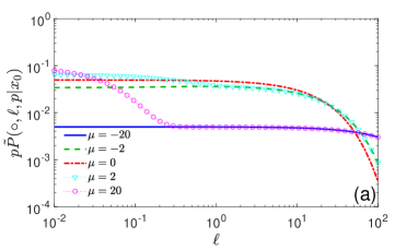
For illustration purposes, we consider the situation when the particle is already on the boundary, so that there is no contribution from the first term in Eq. (85). As the problem is invariant under reflection with respect to the center of the interval (i.e., changing x0x_{0} to Lx0L-x_{0}) along with changing μ\mu to μ-\mu, one can focus on the starting point x0=0x_{0}=0. Figure 3 illustrates the behavior of the probability density P(,,t|0)P(\circ,\ell,t|0) of the boundary local time t\ell_{t}. According to Eq. (85), the Laplace transform of this function reaches a constant as 0\ell\to 0, and rapidly vanishes at large \ell. These properties are preserved in time domain, even though the value of the constant at small \ell depends on time tt. As the short-time limit corresponds to pp\to\infty, the value P~(,0,p|0)\tilde{P}(\circ,0,p|0) weakly depends on the drift, and so does P(,0,t|0)P(\circ,0,t|0), as one can see on the panel (a) for t=0.01t=0.01. Expectedly, the distribution is shifted to the right (towards larger \ell) by a negative drift which keeps the particle in the vicinity of the left endpoint and thus facilitates encounters. In contrast, a positive drift has the opposite effect. At an intermediate time t=0.1t=0.1 (panel (b)), the small-\ell behavior of P(,,t|0)P(\circ,\ell,t|0) is more sensitive to the drift, in particular, the constant plateau at 0\ell\to 0 is strongly attenuated by a strong negative drift (μ=20\mu=-20) because small values of \ell are highly unlikely. A similar trend is also visible for strong positive drift (μ=20\mu=20) which facilitates the passage to the right endpoint. Finally, at moderately long time t=1t=1 (panel (c)), there is almost no difference in the effect of positive and negative drifts. The distribution becomes peaked around the mean value at large drifts μ=±20\mu=\pm 20.

Refer to caption
Refer to caption
Refer to caption
Figure 3: Probability density P(,,t|x0)P(\circ,\ell,t|x_{0}) of the boundary local time t\ell_{t} on the unit interval (L=1L=1), with D=1D=1, x0=0x_{0}=0, and five values of μ\mu (given in the legend) and three values of tt: (a) t=0.01t=0.01, (b) t=0.1t=0.1, and (c) t=1t=1. Vertical dashed lines indicate the corresponding mean boundary local times 𝔼0{t}{\mathbb{E}}_{0}\{\ell_{t}\}. Both P(,,t|x0)P(\circ,\ell,t|x_{0}) and 𝔼0{t}{\mathbb{E}}_{0}\{\ell_{t}\} were obtained via a numerical Laplace transform inversion by a modified Talbot algorithm (see E).

To complete this section, we briefly discuss the probability density pP~(,,p|x0)p\tilde{P}(\circ,\ell,p|x_{0}) of the boundary local time τ\ell_{\tau}, which is stopped at a random time τ\tau with an exponential distribution: {τ>t}=ept{\mathbb{P}}\{\tau>t\}=e^{-pt}. Such a stopping time can describe restricted diffusion in a reactive medium, in which the particle can spontaneously disappear with the rate pp; alternatively, it can describe mortal walkers with a finite lifetime [54, 55]. In this setting, we are interested in the boundary local time at the death moment, i.e., how many times the particle encountered the boundary during its lifetime. According to Eq. (85), the probability density of τ\ell_{\tau} is simply a bi-exponential function, whose decay rates are controlled by the eigenvalues μ±(p)\mu_{\pm}^{(p)}. In this setting, Eq. (85) does not require an inverse Laplace transform anymore and thus allows for a complete, fully explicit and elementary study. We skip this analysis and illustrate the behavior of the probability density on Fig. 4. As previously, a negative drift keeps the particle near the left endpoint and enhances its encounters with that boundary, yielding higher probability for larger values of τ\ell_{\tau}. In turn, a strong positive drift results in two constant levels of the probability density: a higher plateau at small \ell, which corresponds to encounters with the right endpoint, and a lower plateau at larger \ell, which represents the contribution of encounters with the left endpoint (as in the case of the negative drift). In fact, when the particle leaves the left endpoint, it spends a considerable part of its lifetime to diffuse towards the right endpoint, during which the boundary local time does not change. As a consequence, one gets small τ\ell_{\tau} for such realizations. We note that the qualitative behavior for two considered reaction rates p=0.1p=0.1 and p=1p=1 is very similar, except that the decay at large \ell is faster for p=1p=1 because the particles with the shorter lifetime get on average smaller τ\ell_{\tau}.

Refer to caption
Refer to caption
Figure 4: Probability density pP~(,,p|x0)p\tilde{P}(\circ,\ell,p|x_{0}) of the boundary local time τ\ell_{\tau} (stopped at a random time τ\tau exponentially distributed with rate pp) on the unit interval (L=1L=1), with D=1D=1, five values of μ\mu (given in the legend), and two values of the rate pp: (a) p=0.1p=0.1 and (b) p=1p=1.

4 Discussion

In this paper, we extended the encounter-based approach developed in [8] to restricted diffusion with a gradient drift. This approach relies on the Langevin (or Skorokhod) stochastic differential equation that describes simultaneously the position of a particle and its boundary local time. Quite naturally, their joint probability density P(𝒙,,t|𝒙0)P(\bm{x},\ell,t|\bm{x}_{0}), that we called the full propagator, appears to be the fundamental characteristics of restricted diffusion. This quantity is independent of surface reactions and thus properly describes the dynamics alone. In turn, the conventional propagator, which accounts for surface reactions through the Robin boundary condition, can then be deduced as the Laplace transform of P(𝒙,,t|𝒙0)P(\bm{x},\ell,t|\bm{x}_{0}) with respect to the boundary local time \ell. This relation reflects the Bernoulli character of the surface reaction mechanism when the particle attempts to react at each encounter with equal probabilities and these trials are independent from each other. Most importantly, other surface reaction mechanisms can be implemented in a very similar way by replacing the exponential stopping condition. The disentanglement of the diffusive dynamics from surface reactions presents thus one of the major advantages of the encounter-based approach.

In order to derive a spectral decomposition for the Laplace-transformed full propagator, we introduced an appropriate Dirichlet-to-Neumann operator based on the symmetrized version of the Fokker-Planck operator. We illustrated the advantages of this approach in the case of restricted diffusion on an interval with a constant drift. In particular, we analyzed the distribution of the boundary local time and showed the effects of both positive and negative drifts at short and long times. We note that restricted diffusion on the interval (0,L)(0,L) with reflecting endpoints is equivalent to that on an infinite line and on a circle. As a consequence, the obtained exact formula for the distribution of the boundary local time can also describe (i) the boundary local time on discrete points {nL}n\{nL\}_{n\in{\mathbb{Z}}} equally spaced on an infinite line with a periodic triangular potential (see Fig. 5), and (ii) the boundary local time on an even number of equally spaced points on a circle.

Refer to caption
Figure 5: (a) An interval of length LL with two reflecting endpoints and a linearly decreasing potential Φ(x)\Phi(x) that describes a positive drift; (b) An infinite line with equally spaced discrete points {nL}\{nL\} and a triangular periodic potential Φ(x)\Phi(x) that describes alternating positive and negative drifts.

Throughout the manuscript, the whole boundary was supposed to be reactive. In many applications, however, one deals with a reactive region Ω\mathcal{R}\subset\partial\Omega on otherwise inert impermeable boundary, and aims at finding the distribution of first-reaction times on that region. In this case, the Robin boundary condition (8) is replaced by mixed Robin-Neumann boundary condition

jq(𝒔,t|𝒙0)={κGq(𝒔,t|𝒙0)(𝒔),0(𝒔Ω\).j_{q}(\bm{s},t|\bm{x}_{0})=\left\{\begin{array}[]{ll}\kappa G_{q}(\bm{s},t|\bm{x}_{0})&(\bm{s}\in\mathcal{R}),\\ 0&(\bm{s}\in\partial\Omega\backslash\mathcal{R}).\\ \end{array}\right. (87)

As discussed in [53], an extension of the encounter-based approach to this setting is straightforward. In fact, one focuses on the boundary local time on the reactive region \mathcal{R}, which is obtained by substituting Ω\partial\Omega by \mathcal{R} in Eq. (2). The former derivations remain valid, if the definition (36) of the Dirichlet-to-Neumann operator p{\mathcal{M}}_{p} is generalized as

pf=(nw+ϕ(𝒙)w)|,with{(p¯𝒙)w=0(𝒙Ω),w=f(𝒙),nw+ϕ(𝒙)w=0(𝒙Ω\).{\mathcal{M}}_{p}f=\bigl{(}\partial_{n}w+\phi(\bm{x})w\bigr{)}|_{\mathcal{R}},\quad\textrm{with}~{}~{}\left\{\begin{array}[]{ll}(p-\bar{{\mathcal{L}}}_{\bm{x}})w=0&(\bm{x}\in\Omega),\\ w=f&(\bm{x}\in\mathcal{R}),\\ \partial_{n}w+\phi(\bm{x})w=0&(\bm{x}\in\partial\Omega\backslash\mathcal{R}).\end{array}\right. (88)

In other words, the operator p{\mathcal{M}}_{p} associates to a function ff on the reactive region \mathcal{R} another function on \mathcal{R}, keeping the reflecting boundary condition for the solution ww on the remaining inert region Ω\\partial\Omega\backslash\mathcal{R}. Examples of this extension for ordinary diffusion were given in [53]. As the reactive region does not need to be connected, the problem of multiple reactive sites can be treated in this framework. In addition, one can include an absorbing region 𝒜Ω\mathcal{A}\subset\partial\Omega that kills the particle upon the first encounter. In this way, one can investigate surface reactions on \mathcal{R} for a sub-population of particles that avoid hitting 𝒜\mathcal{A}. An implementation of this setting consists in adding the boundary condition w=0w=0 on 𝒜\mathcal{A} in the definition (88) of the Dirichlet-to-Neumann operator (see further discussions in [57]). To get more subtle insights onto reactions on different reactive sites (e.g., competition between them), one can introduce the individual boundary local time on each site and look at their joint distribution [57]. However, appropriate spectral decompositions in this setting are yet unknown.

The proposed encounter-based approach can be further developed in different directions. On one hand, one can dwell on a rigorous proof of the spectral decompositions, on mathematical conditions for the boundary smoothness, on the spectral properties of the introduced extension of the Dirichlet-to-Neumann operator p{\mathcal{M}}_{p}, and on their probabilistic interpretations. In particular, we assumed that p{\mathcal{M}}_{p} is a self-adjoint operator with a discrete spectrum, without discussing eventual limitations on the drift 𝝁(𝒙)\bm{\mu}(\bm{x}). Moreover, one can further extend the present approach to unbounded domains with a compact boundary (e.g., the exterior of a ball). While such an extension was already realized for diffusion without drift (see, e.g., [56]), some limitations on the drift 𝝁(𝒙)\bm{\mu}(\bm{x}) can be expected to ensure the discrete spectrum of the Dirichlet-to-Neumann operator. Yet another mathematical direction is related to the asymptotic analysis of the narrow-escape problem when only a small fraction of the boundary is reactive. On the other hand, one can further explore the advantages of the encounter-based approach for various physical settings. For instance, one can consider the effect of local potentials near the boundary (such as, e.g., electrostatic repulsion or attractive interactions) onto the statistics of boundary encounters. One can consider other surface reaction mechanisms [8] and investigate how the drift may affect them. To some extent, such an approach can provide a microscopic model for so-called intermittent diffusions, in which a particle alternates diffusions in the bulk and on the surface [58, 59, 60, 61, 62, 63, 64, 65, 66, 67]. Similarly, this approach may also help for studying diffusion with reversible binding to the boundary, the so-called sticky boundary condition, when the particle stays on the boundary for a random waiting time and then unbinds to resume its bulk diffusion. The effects of this reversible binding onto reaction rates and first-passage times were thoroughly investigated for ordinary diffusion (see [68, 69, 70, 71, 72] and references therein), as well as for more sophisticated processes such as diffusion with stochastic resetting [73, 74, 75, 76] or velocity jump processes [77, 78, 79, 80, 81]. Since binding to the boundary can be understood as a reaction event on that boundary, the binding time can be described as the first moment when the boundary local time exceeds an exponentially distributed threshold, as in Eq. (13). Changing the probability law for the random threshold allows one to incorporate more sophisticated binding mechanisms (see [8] for details). Curiously, the unbinding event implies resetting of the boundary local time.

Numerous advantages of the encounter-based approach urge for its extensions to even more general diffusion processes, in particular, with general space-dependent drift and volatility matrix. Such an extension would have to overcome two major difficulties.

(i) When the diffusivity varies in the bulk, the reactivity parameter q=κ/Dq=\kappa/D becomes space-dependent as well. As a consequence, the probability of reaction at each encounter depends on the position of that encounter. This dependence would thus prohibit using the Laplace transform relation (16) between the full propagator and the conventional propagator. Following [44], one would thus need to introduce a functional of q(𝑿t)q(\bm{X}_{t}) to account for the cumulative effect of multiple reaction attempts (see also discussion in [57]). Note that a similar difficulty appears in the case of ordinary diffusion towards a heterogeneously reactive boundary, in which case the space-dependent reactivity κ\kappa renders qq to be space-dependent as well [41].

(ii) Even if the diffusivity remains constant, an extension to a general drift becomes challenging. In fact, the Fokker-Planck operator can be reduced to a self-adjoint form with real eigenvalues only in the case of a gradient drift [82]. Even though an appropriate Dirichlet-to-Neumann operator can potentially be introduced in a more general case, such an operator is likely to be non-self-adjoint that would raise considerable challenges in the spectral analysis. Moreover, the numerical computation of the related spectral properties may also be difficult. Nevertheless, further mathematical works in this direction are expected to shed light onto more general diffusion-influenced reactions.

More generally, one can go beyond the framework of stochastic differential equations with Gaussian noises. In the simplest case of random walks on a lattice or a graph, the boundary local time is the number of visits of a given subset of vertices, which can be interpreted as partially reactive sites or localized traps. Szabo et al. showed how to express the related propagator in terms of the propagator without trapping [83]. This concept was recently extended to more general random walks [84]. Another interesting extension concerns diffusion processes with stochastic resetting [73, 74, 75, 76], which can be implemented either for the position, or for the boundary local time, or for both processes. The renewal character of such resettings may allow getting rather explicit results in the Laplace domain. Moreover, the main idea of the encounter-based approach can be potentially applied to other examples of stochastic dynamics such as, e.g., velocity jump processes (including run-and-tumble motion) [77, 78, 79, 80, 81] and continuous-time random walks (including even Lévy flights). However, one would need to properly define the boundary local time (or its analog), as well as an appropriate governing operator (such as the Dirichlet-to-Neumann operator), whose spectral properties would determine the full propagator. Feasibility, mathematical rigor and practical value of such extensions are still open.

The author acknowledges the Alexander von Humboldt Foundation for support within a Bessel Prize award.

Appendix A Auxiliary relation

In this Appendix, we obtain Eq. (46) by extending the derivation from [41].

First, the integral of Eq. (18) over 𝒙Ω\bm{x}\in\Omega yields

pΩ𝑑𝒙G~(𝒙,p|𝒙0)\displaystyle p\int\limits_{\Omega}d\bm{x}\,\tilde{G}_{\infty}(\bm{x},p|\bm{x}_{0}) =\displaystyle= 1+Ω𝑑𝒙(DΔ(𝝁))G~(𝒙,p|𝒙0)\displaystyle 1+\int\limits_{\Omega}d\bm{x}\,(D\Delta-(\nabla\bm{\mu}))\tilde{G}_{\infty}(\bm{x},p|\bm{x}_{0})
=\displaystyle= 1+Ω𝑑𝒙DnG~(𝒙,p|𝒙0).\displaystyle 1+\int\limits_{\partial\Omega}d\bm{x}\,D\partial_{n}\tilde{G}_{\infty}(\bm{x},p|\bm{x}_{0}).

Taking the normal derivative with respect to 𝒙0\bm{x}_{0} at 𝒙0=𝒔0Ω\bm{x}_{0}=\bm{s}_{0}\in\partial\Omega and multiplying by D/p-D/p, we get

Ω𝑑𝒙j~(𝒔0,p|𝒙)=DpΩ𝑑𝒙D(n0nG~(𝒙,p|𝒙0))|𝒙0=𝒔0.\int\limits_{\Omega}d\bm{x}\,\tilde{j}^{\prime}_{\infty}(\bm{s}_{0},p|\bm{x})=-\frac{D}{p}\int\limits_{\partial\Omega}d\bm{x}\,D(\partial_{n_{0}}\partial_{n}\tilde{G}_{\infty}(\bm{x},p|\bm{x}_{0}))|_{\bm{x}_{0}=\bm{s}_{0}}. (89)

Our intention is to exchange the order of normal derivatives in the right-hand side in order to get j~(𝒔0,p|𝒙)\tilde{j}^{\prime}_{\infty}(\bm{s}_{0},p|\bm{x}). However, as this function is singular in the vicinity of 𝒙𝒔0\bm{x}\approx\bm{s}_{0}, one cannot simply exchange the order. To proceed, we use Eq. (26) and evaluate the following derivatives:

n0nG~(𝒙,p|𝒙0)\displaystyle\partial_{n_{0}}\partial_{n}\tilde{G}_{\infty}(\bm{x},p|\bm{x}_{0}) =\displaystyle= n0ne12Φ(𝒙)+12Φ(𝒙0)g~(𝒙,p|𝒙0)\displaystyle\partial_{n_{0}}\partial_{n}e^{-\frac{1}{2}\Phi(\bm{x})+\frac{1}{2}\Phi(\bm{x}_{0})}\tilde{g}_{\infty}(\bm{x},p|\bm{x}_{0})
=\displaystyle= e12Φ(𝒙)+12Φ(𝒙0)(ϕ(𝒙)n0g~(𝒙,p|𝒙0)+n0ng~(𝒙,p|𝒙0)),\displaystyle e^{-\frac{1}{2}\Phi(\bm{x})+\frac{1}{2}\Phi(\bm{x}_{0})}\biggl{(}-\phi(\bm{x})\partial_{n_{0}}\tilde{g}_{\infty}(\bm{x},p|\bm{x}_{0})+\partial_{n_{0}}\partial_{n}\tilde{g}_{\infty}(\bm{x},p|\bm{x}_{0})\biggr{)},
nn0G~(𝒙,p|𝒙0)\displaystyle\partial_{n}\partial_{n_{0}}\tilde{G}_{\infty}(\bm{x},p|\bm{x}_{0}) =\displaystyle= nn0e12Φ(𝒙)+12Φ(𝒙0)g~(𝒙,p|𝒙0)\displaystyle\partial_{n}\partial_{n_{0}}e^{-\frac{1}{2}\Phi(\bm{x})+\frac{1}{2}\Phi(\bm{x}_{0})}\tilde{g}_{\infty}(\bm{x},p|\bm{x}_{0})
=\displaystyle= e12Φ(𝒙)+12Φ(𝒙0)(ϕ(𝒙0)ng~(𝒙,p|𝒙0)+nn0g~(𝒙,p|𝒙0)).\displaystyle e^{-\frac{1}{2}\Phi(\bm{x})+\frac{1}{2}\Phi(\bm{x}_{0})}\biggl{(}\phi(\bm{x}_{0})\partial_{n}\tilde{g}_{\infty}(\bm{x},p|\bm{x}_{0})+\partial_{n}\partial_{n_{0}}\tilde{g}_{\infty}(\bm{x},p|\bm{x}_{0})\biggr{)}.

Since the function g~(𝒙,p|𝒙0)\tilde{g}_{\infty}(\bm{x},p|\bm{x}_{0}) is symmetric, one can exchange the order of normal derivatives. In addition, one has

j~(𝒙,p|𝒙0)\displaystyle\tilde{j}_{\infty}(\bm{x},p|\bm{x}_{0}) =\displaystyle= Dn(e12Φ(𝒙)+12Φ(𝒙0)g~(𝒙,p|𝒙0))\displaystyle-D\partial_{n}\biggl{(}e^{-\frac{1}{2}\Phi(\bm{x})+\frac{1}{2}\Phi(\bm{x}_{0})}\tilde{g}_{\infty}(\bm{x},p|\bm{x}_{0})\biggr{)}
=\displaystyle= ϕ(𝒙)DG~(𝒙,p|𝒙0)De12Φ(𝒙)+12Φ(𝒙0)ng~(𝒙,p|𝒙0),\displaystyle\phi(\bm{x})D\tilde{G}_{\infty}(\bm{x},p|\bm{x}_{0})-De^{-\frac{1}{2}\Phi(\bm{x})+\frac{1}{2}\Phi(\bm{x}_{0})}\partial_{n}\tilde{g}_{\infty}(\bm{x},p|\bm{x}_{0}),
j~(𝒙0,p|𝒙)\displaystyle\tilde{j}^{\prime}_{\infty}(\bm{x}_{0},p|\bm{x}) =\displaystyle= Dn0(e12Φ(𝒙)+12Φ(𝒙0)g~(𝒙,p|𝒙0))\displaystyle-D\partial_{n_{0}}\biggl{(}e^{-\frac{1}{2}\Phi(\bm{x})+\frac{1}{2}\Phi(\bm{x}_{0})}\tilde{g}_{\infty}(\bm{x},p|\bm{x}_{0})\biggr{)}
=\displaystyle= ϕ(𝒙0)DG~(𝒙,p|𝒙0)De12Φ(𝒙)+12Φ(𝒙0)n0g~(𝒙,p|𝒙0).\displaystyle-\phi(\bm{x}_{0})D\tilde{G}_{\infty}(\bm{x},p|\bm{x}_{0})-De^{-\frac{1}{2}\Phi(\bm{x})+\frac{1}{2}\Phi(\bm{x}_{0})}\partial_{n_{0}}\tilde{g}_{\infty}(\bm{x},p|\bm{x}_{0}).

Combining these relations and noting that j~(𝒙,p|𝒙0)=j~(𝒙0,p|𝒙)=δ(𝒙𝒙0)\tilde{j}_{\infty}(\bm{x},p|\bm{x}_{0})=\tilde{j}^{\prime}_{\infty}(\bm{x}_{0},p|\bm{x})=\delta(\bm{x}-\bm{x}_{0}) when both 𝒙\bm{x} and 𝒙0\bm{x}_{0} belong to the boundary Ω\partial\Omega, we get

n0nG~(𝒙,p|𝒙0)nn0G~(𝒙,p|𝒙0)=ϕ(𝒙)+ϕ(𝒙0)Dδ(𝒙𝒙0).\partial_{n_{0}}\partial_{n}\tilde{G}_{\infty}(\bm{x},p|\bm{x}_{0})-\partial_{n}\partial_{n_{0}}\tilde{G}_{\infty}(\bm{x},p|\bm{x}_{0})=\frac{\phi(\bm{x})+\phi(\bm{x}_{0})}{D}\delta(\bm{x}-\bm{x}_{0}). (90)

This relation allows us to rewrite Eq. (89) as

Ω𝑑𝒙j~(𝒔0,p|𝒙)=DpΩ𝑑𝒙(nj~(𝒔0,p|𝒙))2Dϕ(𝒔0)p.\int\limits_{\Omega}d\bm{x}\,\tilde{j}^{\prime}_{\infty}(\bm{s}_{0},p|\bm{x})=\frac{D}{p}\int\limits_{\partial\Omega}d\bm{x}\,(\partial_{n}\tilde{j}^{\prime}_{\infty}(\bm{s}_{0},p|\bm{x}))-\frac{2D\phi(\bm{s}_{0})}{p}. (91)

We multiply both sides of this equation by e12Φ(𝒔0)f(𝒔0)e^{-\frac{1}{2}\Phi(\bm{s}_{0})}f(\bm{s}_{0}) with a suitable function f(𝒔0)f(\bm{s}_{0}) and integrate over 𝒔0Ω\bm{s}_{0}\in\partial\Omega:

Ω𝑑𝒔0e12Φ(𝒔0)f(𝒔0)Ω𝑑𝒙j~(𝒔0,p|𝒙)\displaystyle\int\limits_{\partial\Omega}d\bm{s}_{0}\,e^{-\frac{1}{2}\Phi(\bm{s}_{0})}f(\bm{s}_{0})\int\limits_{\Omega}d\bm{x}\,\tilde{j}^{\prime}_{\infty}(\bm{s}_{0},p|\bm{x})
=DpΩ𝑑𝒔0e12Φ(𝒔0)f(𝒔0){Ω𝑑𝒔(nj~(𝒔0,p|𝒔))2ϕ(𝒔0)}.\displaystyle=\frac{D}{p}\int\limits_{\partial\Omega}d\bm{s}_{0}e^{-\frac{1}{2}\Phi(\bm{s}_{0})}f(\bm{s}_{0})\left\{\int\limits_{\partial\Omega}d\bm{s}\,(\partial_{n}\tilde{j}^{\prime}_{\infty}(\bm{s}_{0},p|\bm{s}))-2\phi(\bm{s}_{0})\right\}. (92)

Our aim is to show that the right-hand side can be represented via the Dirichlet-to-Neumann operator. For this purpose, we note that the solution of the equation (p¯)u=0(p-\bar{{\mathcal{L}}})u=0 with Dirichlet boundary condition u=fu=f on Ω\partial\Omega can be written as

u(𝒙)\displaystyle u(\bm{x}) =\displaystyle= Ω𝑑𝒙0[u(𝒙0)(p¯𝒙0)g~(𝒙,p|𝒙0)g~(𝒙,p|𝒙0)(p¯𝒙0)u(𝒙0)]\displaystyle\int\limits_{\Omega}d\bm{x}_{0}\biggl{[}u(\bm{x}_{0})(p-\bar{{\mathcal{L}}}_{\bm{x}_{0}})\tilde{g}_{\infty}(\bm{x},p|\bm{x}_{0})-\tilde{g}_{\infty}(\bm{x},p|\bm{x}_{0})(p-\bar{{\mathcal{L}}}_{\bm{x}_{0}})u(\bm{x}_{0})\biggr{]}
=\displaystyle= Ω𝑑𝒙0u(𝒙0)(Dn0g~(𝒙,p|𝒙0))\displaystyle\int\limits_{\partial\Omega}d\bm{x}_{0}u(\bm{x}_{0})(-D\partial_{n_{0}}\tilde{g}_{\infty}(\bm{x},p|\bm{x}_{0}))
=\displaystyle= Ω𝑑𝒙0u(𝒙0)(Dn0e12Φ(x)12Φ(𝒙0)G~(𝒙,p|𝒙0))\displaystyle\int\limits_{\partial\Omega}d\bm{x}_{0}u(\bm{x}_{0})(-D\partial_{n_{0}}e^{\frac{1}{2}\Phi(x)-\frac{1}{2}\Phi(\bm{x}_{0})}\tilde{G}_{\infty}(\bm{x},p|\bm{x}_{0}))
=\displaystyle= Ω𝑑𝒔0f(𝒔0)e12Φ(𝒙)12Φ(𝒔0)j~(𝒔0,p|𝒙).\displaystyle\int\limits_{\partial\Omega}d\bm{s}_{0}f(\bm{s}_{0})e^{\frac{1}{2}\Phi(\bm{x})-\frac{1}{2}\Phi(\bm{s}_{0})}\tilde{j}^{\prime}_{\infty}(\bm{s}_{0},p|\bm{x}).

As a consequence, the action of the Dirichlet-to-Neumann operator is

(pf)(𝒔)=ϕ(s)f(𝒔)+(nu)𝒙=𝒔\displaystyle({\mathcal{M}}_{p}f)(\bm{s})=\phi(s)f(\bm{s})+(\partial_{n}u)_{\bm{x}=\bm{s}}
=ϕ(s)f(𝒔)+Ω𝑑𝒔0f(𝒔0)e12Φ(𝒔0)n(e12Φ(𝒙)j~(𝒔0,p|𝒙))|𝒙=𝒔\displaystyle=\phi(s)f(\bm{s})+\int\limits_{\partial\Omega}d\bm{s}_{0}f(\bm{s}_{0})e^{-\frac{1}{2}\Phi(\bm{s}_{0})}\partial_{n}\bigl{(}e^{\frac{1}{2}\Phi(\bm{x})}\tilde{j}^{\prime}_{\infty}(\bm{s}_{0},p|\bm{x})\bigr{)}|_{\bm{x}=\bm{s}}
=ϕ(𝒔)f(𝒔)+Ω𝑑𝒔0f(𝒔0)e12Φ(𝒔0)e12Φ(𝒔)[ϕ(𝒔)j~(𝒔0,p|𝒔)=δ(𝒔𝒔0)+(nj~(𝒔0,p|𝒙))|𝒙=𝒔]\displaystyle=\phi(\bm{s})f(\bm{s})+\int\limits_{\partial\Omega}d\bm{s}_{0}f(\bm{s}_{0})e^{-\frac{1}{2}\Phi(\bm{s}_{0})}e^{\frac{1}{2}\Phi(\bm{s})}\biggl{[}\phi(\bm{s})\underbrace{\tilde{j}^{\prime}_{\infty}(\bm{s}_{0},p|\bm{s})}_{=\delta(\bm{s}-\bm{s}_{0})}+\bigl{(}\partial_{n}\tilde{j}^{\prime}_{\infty}(\bm{s}_{0},p|\bm{x})\bigr{)}|_{\bm{x}=\bm{s}}\biggr{]}
=2ϕ(𝒔)f(𝒔)+Ω𝑑𝒔0f(𝒔0)e12Φ(𝒔0)e12Φ(𝒔)(nj~(𝒔0,p|𝒙))|𝒙=𝒔.\displaystyle=2\phi(\bm{s})f(\bm{s})+\int\limits_{\partial\Omega}d\bm{s}_{0}f(\bm{s}_{0})e^{-\frac{1}{2}\Phi(\bm{s}_{0})}e^{\frac{1}{2}\Phi(\bm{s})}\bigl{(}\partial_{n}\tilde{j}^{\prime}_{\infty}(\bm{s}_{0},p|\bm{x})\bigr{)}|_{\bm{x}=\bm{s}}.

This relation allows us to represent the integral over 𝒔0\bm{s}_{0} in the right-hand side of Eq. (92) in terms of p{\mathcal{M}}_{p}:

Ω𝑑𝒔0e12Φ(𝒔0)f(𝒔0)Ω𝑑𝒙j~(𝒔0,p|𝒙)\displaystyle\int\limits_{\partial\Omega}d\bm{s}_{0}\,e^{-\frac{1}{2}\Phi(\bm{s}_{0})}f(\bm{s}_{0})\int\limits_{\Omega}d\bm{x}\,\tilde{j}^{\prime}_{\infty}(\bm{s}_{0},p|\bm{x})
=Dp{Ωd𝒔e12Φ(𝒔)e12Φ(𝒔)Ω𝑑𝒔0e12Φ(𝒔0)f(𝒔0)(nj~(𝒔0,p|𝒔))=(pf)(𝒔)2ϕ(𝒔)f(𝒔)\displaystyle=\frac{D}{p}\Biggl{\{}\int\limits_{\partial\Omega}d\bm{s}\,e^{-\frac{1}{2}\Phi(\bm{s})}\,\underbrace{e^{\frac{1}{2}\Phi(\bm{s})}\int\limits_{\partial\Omega}d\bm{s}_{0}e^{-\frac{1}{2}\Phi(\bm{s}_{0})}f(\bm{s}_{0})(\partial_{n}\tilde{j}^{\prime}_{\infty}(\bm{s}_{0},p|\bm{s}))}_{=({\mathcal{M}}_{p}f)(\bm{s})-2\phi(\bm{s})f(\bm{s})}
2Ωd𝒔0e12Φ(𝒔0)f(𝒔0)ϕ(𝒔0)},\displaystyle-2\int\limits_{\partial\Omega}d\bm{s}_{0}e^{-\frac{1}{2}\Phi(\bm{s}_{0})}f(\bm{s}_{0})\phi(\bm{s}_{0})\Biggr{\}},

i.e.,

Ω𝑑𝒔0e12Φ(𝒔0)f(𝒔0)Ω𝑑𝒙j~(𝒔0,p|𝒙)=DpΩ𝑑𝒔e12Φ(𝒔)(pf)(𝒔).\int\limits_{\partial\Omega}d\bm{s}_{0}\,e^{-\frac{1}{2}\Phi(\bm{s}_{0})}f(\bm{s}_{0})\int\limits_{\Omega}d\bm{x}\,\tilde{j}^{\prime}_{\infty}(\bm{s}_{0},p|\bm{x})=\frac{D}{p}\int\limits_{\partial\Omega}d\bm{s}\,e^{-\frac{1}{2}\Phi(\bm{s})}({\mathcal{M}}_{p}f)(\bm{s}). (93)

This relation holds for any suitable function f(𝒔)f(\bm{s}) on the boundary. Setting f(𝒔)=vn(p)(𝒔)f(\bm{s})=v_{n}^{(p)}(\bm{s}) to be an eigenfunction of p{\mathcal{M}}_{p}, one gets immediately

Vn(p)¯\displaystyle\overline{V_{n}^{{}^{\prime}(p)}} =\displaystyle= Ω𝑑𝒙Ω𝑑𝒔0e12Φ(𝒔0)vn(p)(𝒔0)j~(𝒔0,p|𝒙)=Vn(p)(𝒙)\displaystyle\int\limits_{\Omega}d\bm{x}\,\underbrace{\int\limits_{\partial\Omega}d\bm{s}_{0}\,e^{-\frac{1}{2}\Phi(\bm{s}_{0})}v_{n}^{(p)}(\bm{s}_{0})\tilde{j}^{\prime}_{\infty}(\bm{s}_{0},p|\bm{x})}_{=V_{n}^{{}^{\prime}(p)}(\bm{x})} (94)
=\displaystyle= Dpμn(p)Ω𝑑𝒔e12Φ(𝒔)vn(p)(𝒔).\displaystyle\frac{D}{p}\mu_{n}^{(p)}\int\limits_{\partial\Omega}d\bm{s}\,e^{-\frac{1}{2}\Phi(\bm{s})}v_{n}^{(p)}(\bm{s}).

Appendix B Green’s functions on the interval

Even though many Green’s functions on the interval are known (see, e.g., [85]), we provide here the main steps of the derivation for the Fokker-Planck operator =Dx2μx{\mathcal{L}}=D\partial_{x}^{2}-\mu\partial_{x} for completeness.

We start with the most general case of Robin boundary conditions at 0 and LL, with two different reactivities q1q_{1} and q2q_{2}. A general solution of the equation (p)u=0(p-{\mathcal{L}})u=0 reads u(x)=c+eα+x+ceαxu(x)=c_{+}e^{\alpha_{+}x}+c_{-}e^{\alpha_{-}x}, with

α±=μ2D±pD+μ24D2,\alpha_{\pm}=\frac{\mu}{2D}\pm\sqrt{\frac{p}{D}+\frac{\mu^{2}}{4D^{2}}}\,, (95)

and two arbitrary coefficients c±c_{\pm}. As usual, one searches for the solution of the equation (18) in the form

G~q1,q2(x,p|x0)={A[(1h1α)eα+x(1h1α+)eαx](0<x<x0),B[(1+h2α)eα+(xL)(1+h2α+)eα(xL)](x0<x<L),\tilde{G}_{q_{1},q_{2}}(x,p|x_{0})=\left\{\begin{array}[]{ll}A\bigl{[}(1-h_{1}\alpha_{-})e^{\alpha_{+}x}-(1-h_{1}\alpha_{+})e^{\alpha_{-}x}\bigr{]}&(0<x<x_{0}),\\ B\bigl{[}(1+h_{2}\alpha_{-})e^{\alpha_{+}(x-L)}-(1+h_{2}\alpha_{+})e^{\alpha_{-}(x-L)}\bigr{]}&(x_{0}<x<L),\\ \end{array}\right. (96)

that satisfies the boundary condition (18) at both endpoints:

(x+q1+μ/D)G~q1,q2(x,p|x0)\displaystyle\bigl{(}-\partial_{x}+q_{1}+\mu/D\bigr{)}\tilde{G}_{q_{1},q_{2}}(x,p|x_{0}) =\displaystyle= 0(x=0),\displaystyle 0\quad(x=0), (97)
(x+q2μ/D)G~q1,q2(x,p|x0)\displaystyle\bigl{(}\partial_{x}+q_{2}-\mu/D\bigr{)}\tilde{G}_{q_{1},q_{2}}(x,p|x_{0}) =\displaystyle= 0(x=L),\displaystyle 0\quad(x=L), (98)

where we set h1=1/(q1+μ/D)h_{1}=1/(q_{1}+\mu/D) and h2=1/(q2μ/D)h_{2}=1/(q_{2}-\mu/D). The unknown coefficients AA and BB are then determined by requiring the continuity of G~q1,q2(x,p|x0)\tilde{G}_{q_{1},q_{2}}(x,p|x_{0}) at x=x0x=x_{0} and the drop of the derivative by 1/D-1/D (i.e., [xG~q1,q2(x,p|x0)]x=x0+ϵ[xG~q1,q2(x,p|x0)]x=x0ϵ1/D[\partial_{x}\tilde{G}_{q_{1},q_{2}}(x,p|x_{0})]_{x=x_{0}+\epsilon}-[\partial_{x}\tilde{G}_{q_{1},q_{2}}(x,p|x_{0})]_{x=x_{0}-\epsilon}\to-1/D as ϵ0\epsilon\to 0):

A\displaystyle A =\displaystyle= eγx0[(1h2γ)sinh(βx¯0)+βh2cosh(βx¯0)]2βD[sinh(βL)(1+γ(h1h2)+(β2γ2)h1h2)+cosh(βL)β(h1+h2)],\displaystyle\frac{e^{\gamma x_{0}}\bigl{[}(1-h_{2}\gamma)\sinh(\beta\bar{x}_{0})+\beta h_{2}\cosh(\beta\bar{x}_{0})\bigr{]}}{2\beta D\bigl{[}\sinh(\beta L)(1+\gamma(h_{1}-h_{2})+(\beta^{2}-\gamma^{2})h_{1}h_{2})+\cosh(\beta L)\beta(h_{1}+h_{2})\bigr{]}}\,, (99)
B\displaystyle B =\displaystyle= eγ(x0L)[(1+h1γ)sinh(βx0)+βh1cosh(βx0)]2βD[sinh(βL)(1+γ(h1h2)+(β2γ2)h1h2)+cosh(βL)β(h1+h2)],\displaystyle-\frac{e^{\gamma(x_{0}-L)}\bigl{[}(1+h_{1}\gamma)\sinh(\beta x_{0})+\beta h_{1}\cosh(\beta x_{0})\bigr{]}}{2\beta D\bigl{[}\sinh(\beta L)(1+\gamma(h_{1}-h_{2})+(\beta^{2}-\gamma^{2})h_{1}h_{2})+\cosh(\beta L)\beta(h_{1}+h_{2})\bigr{]}}\,, (100)

where we used the former notations γ=μ/(2D)\gamma=-\mu/(2D), β=p/D+γ2\beta=\sqrt{p/D+\gamma^{2}}, and x¯0=Lx0\bar{x}_{0}=L-x_{0}. One can also write

G~q1,q2(x,p|x0)={2Aeγx[(1+h1γ)sinh(βx)+h1βcosh(βx)](0<x<x0),2Beγ(xL)[(1h2γ)sinh(βx¯)+h2βcosh(βx¯)](x0<x<L),\tilde{G}_{q_{1},q_{2}}(x,p|x_{0})=\left\{\begin{array}[]{ll}2Ae^{-\gamma x}\bigl{[}(1+h_{1}\gamma)\sinh(\beta x)+h_{1}\beta\cosh(\beta x)\bigr{]}&(0<x<x_{0}),\\ -2Be^{-\gamma(x-L)}\bigl{[}(1-h_{2}\gamma)\sinh(\beta\bar{x})+h_{2}\beta\cosh(\beta\bar{x})\bigr{]}&(x_{0}<x<L),\\ \end{array}\right.

with x¯=Lx\bar{x}=L-x. Setting

U(x)\displaystyle U(x) =\displaystyle= (1+h1γ)sinh(βx)+βh1cosh(βx),\displaystyle(1+h_{1}\gamma)\sinh(\beta x)+\beta h_{1}\cosh(\beta x), (101)
V(x)\displaystyle V(x) =\displaystyle= (1h2γ)sinh(β(Lx))+βh2cosh(β(Lx)),\displaystyle(1-h_{2}\gamma)\sinh(\beta(L-x))+\beta h_{2}\cosh(\beta(L-x)), (102)
C\displaystyle C =\displaystyle= 1βD[sinh(βL)(1+γ(h1h2)+(β2γ2)h1h2)+cosh(βL)β(h1+h2)],\displaystyle\frac{1}{\beta D\bigl{[}\sinh(\beta L)(1+\gamma(h_{1}-h_{2})+(\beta^{2}-\gamma^{2})h_{1}h_{2})+\cosh(\beta L)\beta(h_{1}+h_{2})\bigr{]}}, (103)

one can finally get

G~q1,q2(x,p|x0)=Ceγ(xx0){U(x)V(x0)(0<x<x0),U(x0)V(x)(x0<x<L).\tilde{G}_{q_{1},q_{2}}(x,p|x_{0})=Ce^{-\gamma(x-x_{0})}\left\{\begin{array}[]{ll}U(x)V(x_{0})&(0<x<x_{0}),\\ U(x_{0})V(x)&(x_{0}<x<L).\\ \end{array}\right. (104)

In the particular case of equal reactivities, q1=q2=qq_{1}=q_{2}=q, one has

U(x)\displaystyle U(x) =\displaystyle= U^(x)q2γ,U^(x)=(qγ)sinh(βx)+βcosh(βx),\displaystyle\frac{\hat{U}(x)}{q-2\gamma},\qquad\hat{U}(x)=(q-\gamma)\sinh(\beta x)+\beta\cosh(\beta x),
V(x)\displaystyle V(x) =\displaystyle= V^(x)q+2γ,V^(x)=(q+γ)sinh(β(Lx))+βcosh(β(Lx)),\displaystyle\frac{\hat{V}(x)}{q+2\gamma},\qquad\hat{V}(x)=(q+\gamma)\sinh(\beta(L-x))+\beta\cosh(\beta(L-x)),
C\displaystyle C =\displaystyle= C^q24γ2,C^=1βDsinh(βL)(q2+2βctanh(βL)q+β2γ2).\displaystyle\frac{\hat{C}}{q^{2}-4\gamma^{2}},\qquad\hat{C}=\frac{1}{\beta D\sinh(\beta L)\bigl{(}q^{2}+2\beta\mathrm{ctanh}(\beta L)q+\beta^{2}-\gamma^{2}\bigr{)}}.

More explicitly, one gets

G~q(x,p|x0)\displaystyle\tilde{G}_{q}(x,p|x_{0}) =\displaystyle= eγ(xx0)sinh(βx¯0)sinh(βx)βDsinh(βL)\displaystyle e^{-\gamma(x-x_{0})}\frac{\sinh(\beta\bar{x}_{0})\sinh(\beta x)}{\beta D\sinh(\beta L)}
×\displaystyle\times q2+qβ(ctanh(βx¯0)+ctanh(βx))(γβctanh(βx))(γ+βctanh(βx¯0))q2+2βctanh(βL)q+β2γ2\displaystyle\frac{q^{2}+q\beta(\mathrm{ctanh}(\beta\bar{x}_{0})+\mathrm{ctanh}(\beta x))-(\gamma-\beta\mathrm{ctanh}(\beta x))(\gamma+\beta\mathrm{ctanh}(\beta\bar{x}_{0}))}{q^{2}+2\beta\mathrm{ctanh}(\beta L)q+\beta^{2}-\gamma^{2}}

for 0<x<x00<x<x_{0}, and

G~q(x,p|x0)\displaystyle\tilde{G}_{q}(x,p|x_{0}) =\displaystyle= eγ(xx0)sinh(βx¯)sinh(βx0)βDsinh(βL)\displaystyle e^{-\gamma(x-x_{0})}\frac{\sinh(\beta\bar{x})\sinh(\beta x_{0})}{\beta D\sinh(\beta L)}
×\displaystyle\times q2+qβ(ctanh(βx¯)+ctanh(βx0))(γβctanh(βx0))(γ+βctanh(βx¯))q2+2βctanh(βL)q+β2γ2\displaystyle\frac{q^{2}+q\beta(\mathrm{ctanh}(\beta\bar{x})+\mathrm{ctanh}(\beta x_{0}))-(\gamma-\beta\mathrm{ctanh}(\beta x_{0}))(\gamma+\beta\mathrm{ctanh}(\beta\bar{x}))}{q^{2}+2\beta\mathrm{ctanh}(\beta L)q+\beta^{2}-\gamma^{2}}

for x0<x<Lx_{0}<x<L. Considering this expression as a function qq, one can decompose it into the sum of partial fractions and then perform the inverse Laplace transform with respect to qq in order to get the full propagator. In this way, one can re-derive the general spectral decomposition.

Figure 6 illustrates the behavior of the Green’s function G~q(x,p|x0)\tilde{G}_{q}(x,p|x_{0}) (for visual convenience, this function is multiplied by pp; in fact, for q=0q=0, the integral of this function over xx is equal to 1/p1/p). When μ=1\mu=1, the right wing of G~q(x,p|x0)\tilde{G}_{q}(x,p|x_{0}) is higher, as the positive drift facilitates diffusion to the right.

Refer to caption
Refer to caption
Refer to caption
Refer to caption
Refer to caption
Refer to caption
Figure 6: Green’s function G~q(x,p|x0)\tilde{G}_{q}(x,p|x_{0}) (multiplied by pp) on the unit interval (L=1L=1), with D=1D=1, x0=0.5x_{0}=0.5, several values of pp. Six panels correspond to μ=0\mu=0 (left column) and μ=1\mu=1 (right right) and q=103q=10^{-3} (top row), q=1q=1 (middle row), and q=10q=10 (bottom row).

Appendix C No drift limit

In this Appendix, we briefly describe how the results of Sec. 3 are simplified in the no drift limit.

In the limit μ0\mu\to 0, the eigenvalues of the Dirichlet-to-Neumann operator tend to

μ±(p)=β(cosh(βL)±1)sinh(βL)withβ=p/D,\mu_{\pm}^{(p)}=\frac{\beta(\cosh(\beta L)\pm 1)}{\sinh(\beta L)}\qquad\textrm{with}~{}\beta=\sqrt{p/D}, (105)

while the eigenvectors tend to

v±(p)=12(11),v_{\pm}^{(p)}=\frac{1}{\sqrt{2}}\left(\begin{array}[]{c}1\\ \mp 1\\ \end{array}\right), (106)

so that

V±(p)(x)=V±(p)(x)=sinh(βx¯)sinh(βx)2sinh(βL).V_{\pm}^{(p)}(x)=V_{\pm}^{{}^{\prime}(p)}(x)=\frac{\sinh(\beta\bar{x})\mp\sinh(\beta x)}{\sqrt{2}\sinh(\beta L)}. (107)

In this way, we retrieve the Laplace-transformed full propagator for ordinary diffusion without drift, first derived in [57] 111 There is a misprint in the expression (A.7) from [57]: the sign minus in front of the second term should be replaced by plus, as in Eq. (108).

P~(x,,p|x0)=G~(x,p|x0)δ()+eβctanh(βL)D{sinh(βx¯0)sinh(βx¯)+sinh(βx0)sinh(βx)sinh2(βL)\displaystyle\tilde{P}(x,\ell,p|x_{0})=\tilde{G}_{\infty}(x,p|x_{0})\delta(\ell)+\frac{e^{-\ell\beta\mathrm{ctanh}(\beta L)}}{D}\Biggl{\{}\frac{\sinh(\beta\bar{x}_{0})\sinh(\beta\bar{x})+\sinh(\beta x_{0})\sinh(\beta x)}{\sinh^{2}(\beta L)}
×cosh(βsinh(βL))+sinh(βx¯0)sinh(βx)+sinh(βx0)sinh(βx¯)sinh2(βL)sinh(βsinh(βL))}.\displaystyle\times\cosh\biggl{(}\frac{\beta\ell}{\sinh(\beta L)}\biggr{)}+\frac{\sinh(\beta\bar{x}_{0})\sinh(\beta x)+\sinh(\beta x_{0})\sinh(\beta\bar{x})}{\sinh^{2}(\beta L)}\sinh\biggl{(}\frac{\beta\ell}{\sinh(\beta L)}\biggr{)}\Biggr{\}}. (108)

The marginal probability density of the boundary local time in the Laplace domain reads

P~(,,p|x0)=S~(p|x0)δ()+cosh(βL)1βsinh(βL)=tanh(βL/2)βsinh(βx0)+sinh(βx¯0)sinh(βL)eβtanh(βL/2)D.\tilde{P}(\circ,\ell,p|x_{0})=\tilde{S}_{\infty}(p|x_{0})\delta(\ell)+\underbrace{\frac{\cosh(\beta L)-1}{\beta\sinh(\beta L)}}_{=\frac{\mathrm{tanh}(\beta L/2)}{\beta}}\,\frac{\sinh(\beta x_{0})+\sinh(\beta\bar{x}_{0})}{\sinh(\beta L)}\,\frac{e^{-\beta\mathrm{tanh}(\beta L/2)\ell}}{D}\,. (109)

Appendix D Asymptotic behavior

In this Appendix, we provide technical details for the asymptotic analysis of the short-time and long-time regimes, which correspond to the large-pp and small-pp limits in the Laplace domain, respectively.

D.1 Short-time behavior

Under the condition Lp/D1L\sqrt{p/D}\gg 1, we get βL1\beta L\gg 1 and thus find μ±(p)β±|γ|\mu_{\pm}^{(p)}\approx\beta\pm|\gamma|, with exponentially small corrections. Similarly, we have v+(p)(1,0)v_{+}^{(p)}\approx(1,0)^{\dagger} and v(p)(0,1)v_{-}^{(p)}\approx(0,1)^{\dagger} for μ>0\mu>0, whereas the opposite relations hold for μ<0\mu<0, namely, v+(p)(0,1)v_{+}^{(p)}\approx(0,1)^{\dagger} and v(p)(1,0)v_{-}^{(p)}\approx(1,0)^{\dagger}. As a consequence, we get

V+(p)(x0)eγx0βx0,V(p)(x0)eγx0βx¯0(μ>0),V_{+}^{(p)}(x_{0})\approx e^{\gamma x_{0}-\beta x_{0}}\,,\qquad V_{-}^{(p)}(x_{0})\approx e^{\gamma x_{0}-\beta\bar{x}_{0}}\qquad(\mu>0), (110)

and

V+(p)(x0)eγx0βx¯0,V(p)(x0)eγx0βx0(μ<0).V_{+}^{(p)}(x_{0})\approx e^{\gamma x_{0}-\beta\bar{x}_{0}}\,,\qquad V_{-}^{(p)}(x_{0})\approx e^{\gamma x_{0}-\beta x_{0}}\qquad(\mu<0). (111)

Substituting these expressions into Eq. (48), we get

0𝑑tept𝔼x0{t}1p(e(βγ)x0βγ+e(β+γ)(Lx0)β+γ),\int\limits_{0}^{\infty}dt\,e^{-pt}\,{\mathbb{E}}_{x_{0}}\{\ell_{t}\}\approx\frac{1}{p}\left(\frac{e^{-(\beta-\gamma)x_{0}}}{\beta-\gamma}+\frac{e^{-(\beta+\gamma)(L-x_{0})}}{\beta+\gamma}\right), (112)

whatever the sign of μ\mu. Using the identity

0𝑑teptea2/(4t)(1πtberfcx(a2t+bt))=eapp+b\int\limits_{0}^{\infty}dt\,e^{-pt}\,e^{-a^{2}/(4t)}\left(\frac{1}{\sqrt{\pi t}}-b\,\mathrm{erfcx}\biggl{(}\frac{a}{2\sqrt{t}}+b\sqrt{t}\biggr{)}\right)=\frac{e^{-a\sqrt{p}}}{\sqrt{p}+b} (113)

(here erfcx(x)=ex2(1erf(x))\mathrm{erfcx}(x)=e^{x^{2}}(1-\mathrm{erf}(x)) is the scaled complementary error function), the inverse Laplace transform of Eq. (112) reads

𝔼x0{t}\displaystyle{\mathbb{E}}_{x_{0}}\{\ell_{t}\} \displaystyle\approx 0tdteDγ2t{eγx0[ex02/(4Dt)(Dπt+γDerfcx(x04DtγDt))]\displaystyle\int\limits_{0}^{t}dt^{\prime}\,e^{-D\gamma^{2}t^{\prime}}\left\{e^{\gamma x_{0}}\left[e^{-x_{0}^{2}/(4Dt^{\prime})}\left(\frac{\sqrt{D}}{\sqrt{\pi t^{\prime}}}+\gamma D\,\mathrm{erfcx}\left(\frac{x_{0}}{\sqrt{4Dt^{\prime}}}-\gamma\sqrt{Dt^{\prime}}\right)\right)\right]\right.
+\displaystyle+ eγ(x0L)[e(Lx0)2/(4Dt)(DπtγDerfcx(Lx04Dt+γDt))]}\displaystyle\left.e^{\gamma(x_{0}-L)}\left[e^{-(L-x_{0})^{2}/(4Dt^{\prime})}\left(\frac{\sqrt{D}}{\sqrt{\pi t^{\prime}}}-\gamma D\,\mathrm{erfcx}\left(\frac{L-x_{0}}{\sqrt{4Dt^{\prime}}}+\gamma\sqrt{Dt^{\prime}}\right)\right)\right]\right\}
\displaystyle\approx 0tdt{eγx0[eDγ2tex02/(4Dt)Dπt+γDeγx0erfc(x04DtγDt)]\displaystyle\int\limits_{0}^{t}dt^{\prime}\,\left\{e^{\gamma x_{0}}\left[e^{-D\gamma^{2}t^{\prime}}e^{-x_{0}^{2}/(4Dt^{\prime})}\frac{\sqrt{D}}{\sqrt{\pi t^{\prime}}}+\gamma D\,e^{-\gamma x_{0}}\mathrm{erfc}\left(\frac{x_{0}}{\sqrt{4Dt^{\prime}}}-\gamma\sqrt{Dt^{\prime}}\right)\right]\right.
+\displaystyle+ eγ(Lx0)[eDγ2te(Lx0)2/(4Dt)DπtγDeγ(Lx0)erfc(Lx04Dt+γDt)]}.\displaystyle\left.e^{-\gamma(L-x_{0})}\left[e^{-D\gamma^{2}t^{\prime}}e^{-(L-x_{0})^{2}/(4Dt^{\prime})}\frac{\sqrt{D}}{\sqrt{\pi t^{\prime}}}-\gamma D\,e^{\gamma(L-x_{0})}\mathrm{erfc}\left(\frac{L-x_{0}}{\sqrt{4Dt^{\prime}}}+\gamma\sqrt{Dt^{\prime}}\right)\right]\right\}.

Using the identity

0t𝑑teatb/tt=π2a(e2ab(erf(at+b/t)1)+e2ab(erf(atb/t)+1)),\int\limits_{0}^{t}dt^{\prime}\frac{e^{-at^{\prime}-b/t^{\prime}}}{\sqrt{t^{\prime}}}=\frac{\sqrt{\pi}}{2\sqrt{a}}\biggl{(}e^{2\sqrt{ab}}\biggl{(}\mathrm{erf}(\sqrt{at}+\sqrt{b/t})-1\biggr{)}+e^{-2\sqrt{ab}}\biggl{(}\mathrm{erf}(\sqrt{at}-\sqrt{b/t})+1\biggr{)}\biggr{)},

we get

𝔼x0{t}\displaystyle{\mathbb{E}}_{x_{0}}\{\ell_{t}\} \displaystyle\approx eγx02|γ|[e|γ|x0erfc(x0/4Dt+|γ|Dt)+e|γ|x0erfc(x0/4Dt|γ|Dt)]\displaystyle\frac{e^{\gamma x_{0}}}{2|\gamma|}\biggl{[}-e^{|\gamma|x_{0}}\mathrm{erfc}(x_{0}/\sqrt{4Dt}+|\gamma|\sqrt{Dt})+e^{-|\gamma|x_{0}}\mathrm{erfc}(x_{0}/\sqrt{4Dt}-|\gamma|\sqrt{Dt})\biggr{]}
+\displaystyle+ eγx¯02|γ|[e|γ|x¯0erfc(x¯0/4Dt+|γ|Dt)+e|γ|x¯0erfc(x¯0/4Dt|γ|Dt)]\displaystyle\frac{e^{-\gamma\bar{x}_{0}}}{2|\gamma|}\biggl{[}-e^{|\gamma|\bar{x}_{0}}\mathrm{erfc}(\bar{x}_{0}/\sqrt{4Dt}+|\gamma|\sqrt{Dt})+e^{-|\gamma|\bar{x}_{0}}\mathrm{erfc}(\bar{x}_{0}/\sqrt{4Dt}-|\gamma|\sqrt{Dt})\biggr{]}
+\displaystyle+ γD0t𝑑t{erfc(x04DtγDt)erfc(x¯04Dt+γDt)}.\displaystyle\gamma D\int\limits_{0}^{t}dt^{\prime}\biggl{\{}\mathrm{erfc}\biggl{(}\frac{x_{0}}{\sqrt{4Dt^{\prime}}}-\gamma\sqrt{Dt^{\prime}}\biggr{)}-\mathrm{erfc}\biggl{(}\frac{\bar{x}_{0}}{\sqrt{4Dt^{\prime}}}+\gamma\sqrt{Dt^{\prime}}\biggr{)}\biggr{\}}.

In particular, for x0=0x_{0}=0, we get after simplifications

𝔼0{t}1γ(erf(γDt)2+γ2Dterfc(γDt)|γ|DtπeDγ2t).{\mathbb{E}}_{0}\{\ell_{t}\}\approx\frac{1}{\gamma}\left(\frac{\mathrm{erf}(\gamma\sqrt{Dt})}{2}+\gamma^{2}Dt\,\mathrm{erfc}(-\gamma\sqrt{Dt})-\frac{|\gamma|\sqrt{Dt}}{\sqrt{\pi}}\,e^{-D\gamma^{2}t}\right). (114)

D.2 Long-time behavior

Let us consider the case γ0\gamma\neq 0. In the limit p0p\to 0, we get up to O(p2)O(p^{2}):

β\displaystyle\beta \displaystyle\approx |γ|+p2|γ|D,\displaystyle|\gamma|+\frac{p}{2|\gamma|D}\,,
μ±(p)\displaystyle\mu_{\pm}^{(p)} \displaystyle\approx |γ|ctanh(|γ|L)(1+p2γ2DpL|γ|Dsinh(2|γ|L))\displaystyle|\gamma|\mathrm{ctanh}(|\gamma|L)\biggl{(}1+\frac{p}{2\gamma^{2}D}-\frac{pL}{|\gamma|D\sinh(2|\gamma|L)}\biggr{)}
±\displaystyle\pm |γ|ctanh(|γ|L)(1+12cosh2(|γ|L)(pDγ2pL|γ|Dctanh(|γ|L))),\displaystyle|\gamma|\mathrm{ctanh}(|\gamma|L)\biggl{(}1+\frac{1}{2\cosh^{2}(|\gamma|L)}\biggl{(}\frac{p}{D\gamma^{2}}-\frac{pL}{|\gamma|D}\mathrm{ctanh}(|\gamma|L)\biggr{)}\biggr{)}\,,

so that

μ(p)\displaystyle\mu_{-}^{(p)} \displaystyle\approx ptanh(γL)2γD+O(p2),\displaystyle p\frac{\mathrm{tanh}(\gamma L)}{2\gamma D}+O(p^{2}),
μ+(p)\displaystyle\mu_{+}^{(p)} \displaystyle\approx 2γctanh(γL)+O(p).\displaystyle 2\gamma\mathrm{ctanh}(\gamma L)+O(p).

We also have

(p)11\displaystyle({\mathcal{M}}_{p})_{11} \displaystyle\approx γctanh(γL)(1+p2γ2DpLγDsinh(2γL))γ,\displaystyle\gamma\mathrm{ctanh}(\gamma L)\left(1+\frac{p}{2\gamma^{2}D}-\frac{pL}{\gamma D\sinh(2\gamma L)}\right)-\gamma,
(p)12\displaystyle({\mathcal{M}}_{p})_{12} \displaystyle\approx γsinh(γL)(1+p2γ2DpLctanh(γL)2γD).\displaystyle-\frac{\gamma}{\sinh(\gamma L)}\left(1+\frac{p}{2\gamma^{2}D}-\frac{pL\mathrm{ctanh}(\gamma L)}{2\gamma D}\right).

In the lowest order, we also get

v(p)(0)\displaystyle v_{-}^{(p)}(0) \displaystyle\approx 1cosh(γL)2(1tanh(γL))+O(p),\displaystyle\frac{1}{\cosh(\gamma L)\sqrt{2(1-\mathrm{tanh}(\gamma L))}}+O(p),
v(p)(L)\displaystyle v_{-}^{(p)}(L) \displaystyle\approx (1tanh(γL))/2+O(p).\displaystyle\sqrt{(1-\mathrm{tanh}(\gamma L))/2}+O(p).

Substituting these expressions into Eq. (76) for x0x_{0}, we deduce in the leading order

0𝑑tept𝔼0{t}=2γDctanh(γL)p2+O(1/p),\int\limits_{0}^{\infty}dt\,e^{-pt}\,{\mathbb{E}}_{0}\{\ell_{t}\}=\frac{2\gamma D\mathrm{ctanh}(\gamma L)}{p^{2}}+O(1/p), (115)

from which Eq. (77) follows immediately.

Appendix E On the numerical inversion of the Laplace transform

The inverse Laplace transform f(t)f(t) of a function f~(p)\tilde{f}(p) can be expressed as the Bromwich integral,

f(t)=12πiγ𝑑peptf~(p),f(t)=\frac{1}{2\pi i}\int\limits_{\gamma}dp\,e^{pt}\,\tilde{f}(p), (116)

where γ\gamma is a contour from i-i\infty to +i+i\infty in the complex plane that lies on the right to singularities of f~(p)\tilde{f}(p). In the basic Talbot algorithm, the contour γ\gamma is parameterized as

γ:θp(θ)=σ+μ(θctan(θ)+νiθ),θ(π,π),\gamma~{}:~{}\theta\to p(\theta)=\sigma+\mu(\theta\mathrm{ctan}(\theta)+\nu i\theta),\qquad\theta\in(-\pi,\pi), (117)

with three parameters σ\sigma, μ\mu and ν\nu whose optimal choice depends on the function f~(p)\tilde{f}(p) and determines the convergence rate [86]. Using this contour, the Bromwich integral can be reduced to

f(t)=12πiππ𝑑θdpdθep(θ)tf~(p(θ)),f(t)=\frac{1}{2\pi i}\int\limits_{-\pi}^{\pi}d\theta\,\frac{dp}{d\theta}\,e^{p(\theta)t}\,\tilde{f}(p(\theta)), (118)

and then numerically evaluated by quadratures. In this paper, we used a slightly different contour by Weideman [87]:

γ:θp(θ)=N(0.5017θctan(0.6407θ)0.6122+0.2645iθ),θ(π,π),\gamma~{}:~{}\theta\to p(\theta)=N\bigl{(}0.5017\,\theta\,\mathrm{ctan}(0.6407\,\theta)-0.6122+0.2645i\,\theta),\quad\theta\in(-\pi,\pi), (119)

where the value of NN controls the accuracy of computation.


References

  • [1] Carslaw HS and Jaeger JC (1959) Conduction of Heat in Solids, 2nd Ed. (Clarendon, Oxford)
  • [2] Risken H (1996) The Fokker-Planck equation: methods of solution and applications, 3rd Ed. (Berlin: Springer)
  • [3] Gardiner CW (1983) Handbook of Stochastic Methods for Physics, Chemistry and the Natural Sciences (Berlin: Springer-Verlag)
  • [4] Redner S (2001) A Guide to First Passage Processes (Cambridge: Cambridge University press)
  • [5] Schuss Z (2013) Brownian Dynamics at Boundaries and Interfaces in Physics, Chemistry and Biology (Springer, New York)
  • [6] Metzler R, Oshanin G, and Redner S (2014) First-Passage Phenomena and Their Applications (World Scientific Press, Singapore)
  • [7] Lindenberg K, Metzler R, and Oshanin G (2019) Chemical Kinetics: Beyond the Textbook (World Scientific, New Jersey)
  • [8] Grebenkov DS (2020) Phys. Rev. Lett. 125 078102
  • [9] Lévy P (1965) Processus Stochastiques et Mouvement Brownien (Paris, Gauthier-Villard)
  • [10] Itô K and McKean HP (1965) Diffusion Processes and Their Sample Paths (Springer-Verlag, Berlin)
  • [11] Freidlin M (1985) Functional Integration and Partial Differential Equations (Annals of Mathematics Studies, Princeton University Press, Princeton, New Jersey)
  • [12] Darling DA and Kac M (1957) Trans. Am. Math. Soc. 84 444-458
  • [13] Ray D (1963) Illinois J. Math. 7 615
  • [14] Knight FB (1963) Trans. Amer. Math. Soc. 109 56-86
  • [15] Agmon N (1984) J. Chem. Phys. 81 3644
  • [16] Berezhkovskii AM, Zaloj V, and Agmon N (1998) Phys. Rev. E 57 3937
  • [17] Dhar A and Majumdar SN (1999) Phys. Rev. E 59 6413
  • [18] Yuste SB and Acedo L (2001) Phys. Rev. E 64 061107
  • [19] Godrèche C and Luck JM (2001) J. Stat. Phys. 104 489
  • [20] Majumdar SN and Comtet A (2002) Phys. Rev. Lett. 89 060601
  • [21] Bénichou O, Coppey M, Klafter J, Moreau M, and Oshanin G (2003) J. Phys. A.: Math. Gen. 36 7225-7231
  • [22] Condamin S, Bénichou O, and Moreau M (2005) Phys. Rev. E 72 016127
  • [23] Condamin S, Tejedor V, and Bénichou O (2007) Phys. Rev. E 76 050102R
  • [24] Burov S and Barkai E (2007) Phys. Rev. Lett. 98 250601
  • [25] Burov S and Barkai E (2011) Phys. Rev. Lett. 107 170601
  • [26] Collins FC and Kimball GE (1949) J. Coll. Sci. 4 425.
  • [27] Sano H and Tachiya M (1979) J. Chem. Phys. 71 1276-1282
  • [28] Shoup D and Szabo A (1982) Biophys. J. 40 33-39
  • [29] Zwanzig R (1990) Proc. Natl. Acad. Sci. USA 87 5856
  • [30] Sapoval B (1994) Phys. Rev. Lett. 73 3314-3317
  • [31] Filoche M and Sapoval B (1999) Eur. Phys. J. B 9 755-763
  • [32] Bénichou O, Moreau M, and Oshanin G (2000) Phys. Rev. E 61 3388-3406
  • [33] Grebenkov DS, Filoche M, and Sapoval B (2003) Eur. Phys. J. B 36 221-231
  • [34] Berezhkovskii A, Makhnovskii Y, Monine M, Zitserman V, and Shvartsman S (2004) J. Chem. Phys. 121 11390
  • [35] Grebenkov DS (2006) Partially Reflected Brownian Motion: A Stochastic Approach to Transport Phenomena, in “Focus on Probability Theory”, Ed. L. R. Velle, pp. 135-169 (Nova Science Publishers).
  • [36] Grebenkov DS, Filoche M, and Sapoval B (2006) Phys. Rev. E 73 021103
  • [37] Reingruber J and Holcman D (2009) Phys. Rev. Lett. 103 148102
  • [38] Lawley S and Keener JP (2015) SIAM J. Appl. Dyn. Sys. 14 1845-1867
  • [39] Grebenkov DS and Oshanin G (2017) Phys. Chem. Chem. Phys. 19 2723-2739
  • [40] Bernoff A, Lindsay A, and Schmidt D (2018) Multiscale Model. Simul. 16 1411-1447
  • [41] Grebenkov DS J. Chem. Phys. 151 104108
  • [42] Mörters P and Peres Y (2010) Brownian Motion (Cambridge Series in Statistical and Probabilistic Mathematics, Cambridge University Press, Cambridge)
  • [43] Grebenkov DS (2007) Phys. Rev. E 76 041139
  • [44] Papanicolaou VG (1990) Probab. Th. Rel. Fields 87 27-77
  • [45] Arendt W, ter Elst AFM, Kennedy JB, and Sauter M (2014) J. Funct. Anal. 266 1757-1786
  • [46] Daners D (2014) Positivity 18 235-256
  • [47] ter Elst AFM and Ouhabaz EM (2014) J. Funct. Anal. 267 4066-4109
  • [48] Behrndt J and ter Elst AFM (2015) J. Diff. Eq. 259 5903-5926
  • [49] Arendt W and ter Elst AFM (2015) Potential Anal. 43 313-340
  • [50] Hassell A and Ivrii V (2017) J. Spectr. Theory 7 881-905
  • [51] Girouard A and Polterovich I (2017) J. Spectr. Theory 7 321-359
  • [52] Grebenkov DS (2019) Phys. Rev. E 100 062110
  • [53] Grebenkov DS (2020) Phys. Rev. E 102 032125
  • [54] Meerson B and Redner S (2015) Phys. Rev. Lett. 114 198101
  • [55] Grebenkov DS and Rupprecht J-F (2017) J. Chem. Phys. 146 084106
  • [56] Grebenkov DS (2021) J. Phys. A.: Math. Theor. 54 015003
  • [57] Grebenkov DS (2020) J. Stat. Mech. 103205 (2020).
  • [58] Levitz PE, Zinsmeister M, Davidson P, Constantin D, and Poncelet O (2008) Phys. Rev. E 78 030102(R)
  • [59] Chechkin AV, Zaid IM, Lomholt MA, Sokolov IM, and Metzler R (2009) Phys. Rev. E 79 040105(R)
  • [60] Bénichou O, Grebenkov DS, Levitz P, Loverdo C, and Voituriez R (2010) Phys. Rev. Lett. 105 150606
  • [61] Bénichou O, Grebenkov DS, Levitz P, Loverdo C, and Voituriez R (2011) J. Stat. Phys. 142 657-685
  • [62] Chechkin AV, Zaid IM, Lomholt MA, Sokolov IM, and Metzler R (2011) J. Chem. Phys. 134 204116
  • [63] Chechkin AV, Zaid IM, Lomholt MA, SokolovIM, and Metzler R (2012) Phys. Rev. E 86 041101
  • [64] Rupprecht J-F, Bénichou O, Grebenkov DS, and Voituriez R (2012) J. Stat. Phys. 147 891-918
  • [65] Rupprecht J-F, Bénichou O, Grebenkov DS, and Voituriez R (2012) Phys. Rev. E 86 041135
  • [66] Berezhkovskii AM, Dagdug L, and Bezrukov SM (2015) J. Chem. Phys. 143 084103
  • [67] Berezhkovskii AM, Dagdug L, and Bezrukov SM (2017) J. Chem. Phys. 147 014103
  • [68] Agmon N and Szabo A (1990) J. Chem. Phys. 92 5270
  • [69] Prüstel T and Tachiya M (2013) J. Chem. Phys. 139 194103
  • [70] Grebenkov DS (2017) J. Chem. Phys. 147 134112
  • [71] Lawley SD and Madrid JB (2019) J. Chem. Phys. 150 214113
  • [72] Reva M, DiGregorio DA, and Grebenkov DS (2021) Sci. Rep. 11 5377
  • [73] Evans MR and Majumdar SN (2011) Phys. Rev. Lett. 106 160601
  • [74] Chechkin A and Sokolov IM (2018) Phys. Rev. Lett. 121 050601
  • [75] Evans MR and Majumdar SN (2019) J. Phys. A: Math. Theor. 52 01LT01
  • [76] Evans MR, Majumdar SN, and Schehr G (2020) J. Phys. A: Math. Theor. 53 193001
  • [77] Gopalakrishnan M and Govindan BS (2011) Bull. Math. Biol. 73 2483-2506
  • [78] Zelinski B, Muller N, and Kierfeld J (2012) Phys. Rev. E 86 041918
  • [79] Mulder BM (2012) Phys. Rev. E 86 011902
  • [80] Angelani L J. Phys. A: Math. Theor. 50 325601
  • [81] Bressloff PC and Kim H (2019) Phys. Rev. E 99 052401
  • [82] Nelson E (1958) Duke Math. J. 25 671-690
  • [83] Szabo A, Lamm G, and Weiss GH (1984) J. Stat. Phys. 34 225-238
  • [84] Guérin T, Dolgushev M, Bénichou O, and Voituriez R (2021) Commun. Chem. 4 157
  • [85] Thambynayagam RKM (2011) The Diffusion Handbook: Applied Solutions for Engineers (New York: McGraw-Hill Education)
  • [86] Talbot A (1979) J. Inst. Maths. Applics. 23 97-120
  • [87] Weideman JAC (2006) SIAM J. Num. Anal. 44 2342-2362