An efficient proximal-based approach for solving nonlocal Allen-Cahn equations

Olena Burkovska¹ and Ilyas Mustapha² ¹ Computer Science and Mathematics Division, Oak Ridge National Laboratory, USA [email protected] ² Department of Mathematics, Kansas State University, Manhattan, KS, USA [email protected]

Abstract.

In this work, we present an efficient approach for the spatial and temporal discretization of the nonlocal Allen-Cahn equation, which incorporates various double-well potentials and an integrable kernel, with a particular focus on a non-smooth obstacle potential. While nonlocal models offer enhanced flexibility for complex phenomena, they often lead to increased computational costs and there is a need to design efficient spatial and temporal discretization schemes, especially in the non-smooth setting. To address this, we propose first- and second-order energy-stable time-stepping schemes combined with the Fourier collocation approach for spatial discretization. We provide energy stability estimates for the developed time-stepping schemes. A key aspect to our approach involves a representation of a solution via proximal operators. This together with the spatial and temporal discretizations enables direct evaluation of the solution that can bypass the solution of nonlinear, non-smooth, and nonlocal system. This method significantly improves computational efficiency, especially in the case of non-smooth obstacle potentials, and facilitates rapid solution evaluations in both two and three dimensions. We provide several numerical experiments to illustrate the effectiveness of our approach.

Key words and phrases:

phase-field models, nonlocal operators, proximal operators, variational inequalities, FFT, energy stability

2010 Mathematics Subject Classification:

45K05; 35K55; 35B65; 49J40; 65M60; 65K15

This material is based upon work supported by the National Science Foundation MSGI program and the U.S. Department of Energy, Office of Advanced Scientific Computing Research, Applied Mathematics Program under the award numbers ERKJ345; and was performed at the Oak Ridge National Laboratory, which is managed by UT-Battelle, LLC under Contract No. De-AC05-00OR22725. The US government retains and the publisher, by accepting the article for publication, acknowledges that the US government retains a nonexclusive, paid-up, irrevocable, worldwide license to publish or reproduce the published form of this manuscript, or allow others to do so, for US government purposes. DOE will provide public access to these results of federally sponsored research in accordance with the DOE Public Access Plan (https://www.energy.gov/doe-public-access-plan).

1. Introduction

Phase-field models, such as Allen-Cahn and Cahn-Hilliard, are widely used to describe phase-transition phenomena in various applications, including solidification in materials science [38, 47], image processing [9], and mean-curvature flow [20]. Typically, local phase-field models, based on partial derivatives, are considered. However, incorporating nonlocality in phase-field modeling enhances versatility for capturing anomalous processes and is better suited to describe sharp interfaces. Unlike local models, nonlocal models rely on integral operators with a nonlocal kernel that accounts for long-range interactions. While nonlocal settings provide greater modeling flexibility, they often require more careful numerical treatment to develop efficient methods for discretizing the integral operator.

In this work, we propose an efficient discretization of the nonlocal Allen-Cahn equation with various potential functions, including regular, singular (Flory-Huggins or logarithmic), and obstacle potentials. This encompasses a broad range of models, from nonlinear to nonlinear non-smooth types. Our method is based on characterizing the solution using the proximal operator, combined with efficient evaluation of the convolution through fast Fourier transform (FFT). In contrast to existing methods, our approach can handle a wide variety of non-smooth or singular potentials without the need for additional approximations, such as regularizing the logarithmic potential [31] or using Moreau-Yosida regularization for the obstacle potential [32, 36].

More specifically, we consider the model of the following form:

\partial_{t}u+\mathcal{L}u+\partial F(u)\ni 0,\quad\text{ in }(0,T)\times\Omega,

(1.1)

where $\Omega\subset\mathbb{R}^{n}$ , $n\leq 3$ , is a bounded domain, $T>0$ is a fixed time, and the model is supplemented with a suitable initial condition and periodic boundary conditions. The operator $\mathcal{L}\colon L^{2}(\Omega)\to L^{2}(\Omega)$ is a nonlocal diffusion operator defined as

\displaystyle\mathcal{L}u(x)=\int_{\Omega}(u(x)-u(y))\gamma(x-y)\mathop{}\!\mathrm{d}y=c_{\gamma}u(x)-(\gamma*u)(x),\quad c_{\gamma}>0,

(1.2)

where $c_{\gamma}=(\gamma*1)=\int_{\Omega}\gamma(x-y)\mathop{}\!\mathrm{d}y$ and $\gamma\colon\Omega\to\mathbb{R}$ is an integrable convolution kernel that sets up the law and extend of nonlocal interactions. The nonlocal energy associated with (1.1) has the following form:

\mathcal{E}(u):=\frac{1}{4}\int_{\Omega}\int_{\Omega}(u(x)-u(y))^{2}\gamma(x-y)\mathop{}\!\mathrm{d}x\mathop{}\!\mathrm{d}y+\int_{\Omega}F(u)\mathop{}\!\mathrm{d}x,

(1.3)

which is an analogue of the local Ginzburg-Landau energy.

Here, $F$ is a double-well potential that attains two local minima when the phase-field variable $u$ is at pure phases $\pm 1$ (e.g., solid and liquid) and is the driving force of the phase-separation encouraging the solution to attain pure phases. More specifically, we set

F(u)=f_{0}(u)+\psi(u),

(1.4)

where $f_{0}\colon\mathbb{R}\to\mathbb{R}$ is concave differentiable part of $F$ and $\psi\colon\mathbb{R}\to\mathbb{R}\cup\{\infty\}$ is a (potentially non-differentiable) convex lower semi-continuous function. Three common types of double-well potentials: regular, logarithmic (Flory-Huggins) and obstacle, can be expressed in the form of (1.4) with

f_{0}(u)=\frac{c_{F}}{2}(1-u^{2}),\quad c_{F}>0,

(1.5)

and $\psi$ to be defined for the obstacle potential by a convex indicator function:

\psi_{\rm obs}(u)=\mathbb{I}_{[-1,1]}(u)=\begin{cases}0,\leavevmode\nobreak\ \text{ if }u\in[-1,1]\\ +\infty,\text{ otherwise}\end{cases},

(1.6)

for the logarithmic (Flory-Huggins) potential¹¹1Here, the values at $u=\pm 1$ are defined by the limit of the function that leads to $\frac{\theta_{c}}{2}\ln(2)$ . by

\psi_{\rm log}(u)=\ \begin{cases}\frac{\theta_{c}}{2}\left((1+u)\ln(1+u)+(1-u)\ln(1-u)\right),\quad\text{if}\;u\in[-1,1],\\ +\infty,\quad\text{otherwise},\end{cases}

(1.7)

with $0<\theta_{c}<c_{F}$ and for the regular potential by

\displaystyle\psi_{\rm reg}(u)=\frac{c_{F}}{4}\left(u^{4}-1\right),\quad c_{F}>0.

(1.8)

The corresponding generalized subdifferential (1.9) is then defined as follows

\partial F(u)=f_{0}^{\prime}(u)+\partial\psi(u)=-c_{F}u+\partial\psi(u),

(1.9)

with the subdifferential $\partial\psi(u)$ being


$\displaystyle\partial\psi_{\rm obs}=$	$\displaystyle\ \partial\mathbb{I}_{[-1,1]}(u):=\begin{cases}(-\infty,0],&u=-1,\\ 0,&u\in(-1,1),\\ [0,\infty),&u=1,\end{cases}$	(1.10a)
$\displaystyle\partial\psi_{\rm log}=$	$\displaystyle\begin{cases}\emptyset,&u\not\in[-1,1],\\ \left\{\frac{\theta_{c}}{2}\left(\ln(1+u)-\ln(1-u)\right)\right\},&u\in(-1,1),\end{cases}$	(1.10b)
$\displaystyle\partial\psi_{\rm reg}=$	$\displaystyle\ \{c_{F}u^{3}\}.$	(1.10c)

Using the definitions (1.2) and (1.9), the equation (1.1) transforms to:

\displaystyle\partial_{t}u+\xi u-\gamma*u+\partial\psi(u)\ni 0,

(1.11)

where $\xi=c_{\gamma}-c_{F}\geq 0$ is a nonlocal interface parameter that defines the width of the transition region between pure phases.

A notable feature of nonlocal models is that they are more naturally suited to describe sharp-interface dynamics, see, e.g., [6, 7, 15, 17, 18, 22, 23, 24, 25, 39] and the references cited therein. In particular, the nonlocal Allen-Cahn and Cahn-Hilliard models allow for well-defined sharp-interfaces in the solution at steady state and transient times, respectively. Unlike the corresponding local models, where sharp interfaces in the solution are achieved only in the asymptotic case of vanishing local interface parameter, nonlocal framework provides more natural and well-defined description to model discontinuous profiles in the solution. The choice of a double-well potential function greatly influences the interface sharpness. In particular, for $\xi=0$ an obstacle potential can lead to solutions with perfectly sharp interfaces, with jump discontinuities in the solution, representing pure phases with no intermediate transitions [15, 17], while a regular potential for $\xi<0$ results in interfaces that, although discontinuous, may exhibit a narrow transition region between phases [23]. To illustrate this, we plot on Figure 1.1 various potentials and the corresponding solutions of (1.1) close to a steady-state. We observe that the obstacle potential yields the sharpest interface, while the regular potential results in a more diffuse one. For the Flory-Huggins potential, the sharpness of the interface is influenced by the parameter $\theta_{c}$ ; specifically, smaller values of $\theta_{c}$ produce a sharper interface, as a decrease in $\theta_{c}$ causes the logarithmic potential to approach the non-smooth obstacle potential.

The sharp interface property is inherent to the structure of the model (1.1), which we are also going to explore to design efficient temporal and spatial discretizations and solution strategies. Specifically, exploiting (1.1) and the potential (1.4), we can derive a representation formula for the solution using proximal operators, as detailed below. This representation enables simplified and efficient computation of the solution, in some cases completely eliminating the need to solve nonlinear and non-smooth systems.

1.1. Representation formula

We discuss briefly, how one can characterize the time-discrete solution of (1.11) in terms of the proximal operators and derivation of the representation formula. Employing a semi-implicit Euler time-stepping scheme (more details on this and higher order schemes are discussed in Section 2) with an explicit discretization of the convolution to (1.11) leads to:

\frac{1}{\Delta t}\left(u^{k}-u^{k-1}\right)+\xi u^{k}-\gamma*u^{k-1}+\partial\psi(u^{k})\ni 0,

(1.12)

with $k=1,\dots,K$ , $\Delta t=T/K$ , $K\in\mathbb{N}$ , which is also equivalent to

u^{k}={\rm prox}_{\frac{1}{\lambda}\psi}\left(\frac{1}{\lambda}\left(\gamma*u^{k-1}+\frac{1}{\Delta t}u^{k-1}\right)\right),

(1.13)

with $\lambda=\xi+1/\Delta t>0$ . Here, ${\rm prox}_{\frac{1}{\lambda}\psi}\colon\mathbb{R}\to\mathbb{R}$ is a proximal operator of $\frac{1}{\lambda}\psi$ [8, 14]: defined as

{\rm prox}_{\frac{1}{\lambda}\psi}(v)=\operatorname{arg\min}_{s}\left(\frac{1}{\lambda}\psi(s)+\frac{1}{2}|s-v|^{2}\right),

which is also related to the subdifferential $\partial\psi$ as

{\rm prox}_{\frac{1}{\lambda}\psi}=\left(I+\frac{1}{\lambda}\partial\psi\right)^{-1},\quad\lambda=1/\Delta t+\xi>0.

(1.14)

Here, the relation (1.13) should be understood pointwise, in a sense that $u^{k}(x)={\rm prox}_{\frac{1}{\lambda}\psi}(g^{k}(x)/\lambda)$ with $g^{k}(x)=(\gamma*u^{k-1})(x)+\frac{1}{\Delta t}u^{k-1}(x)$ for $x\in\Omega$ .

The representaton (1.13) provides a useful approach from a computational standpoint. Knowing the proximal operator one can directly evaluate the solution at each time step using its values from the previous time step. In particular, for the case of an obstacle potential ( $\psi(u)=\mathbb{I}_{[-1,1]}(u)$ ), the proximal operator reduces to the pointwise projection operator and (1.13) becomes

u^{k}=P_{[-1,1]}\left(\frac{1}{\lambda}\left(\gamma*u^{k-1}+\frac{1}{\Delta t}u^{k-1}\right)\right).

(1.15)

For the case of a regular potential, the proximal operator is computed by using Cardano’s formula [48] and (1.13) becomes

u^{k}={\rm prox}_{\frac{1}{\lambda}\psi}\left(\frac{1}{\lambda}\zeta_{k}\right)=\sqrt[3]{\tilde{\zeta}_{k}+\sqrt{\tilde{\zeta}_{k}^{2}+\left({\lambda}/{3c_{F}}\right)^{3}}}+\sqrt[3]{\tilde{\zeta}_{k}-\sqrt{\tilde{\zeta}_{k}^{2}+\left({\lambda}/{3c_{F}}\right)^{3}}},

(1.16)

where $\zeta_{k}=\left(\gamma*u^{k-1}+\frac{1}{\Delta t}u^{k-1}\right)$ and $\tilde{\zeta}_{k}=\zeta_{k}/(2c_{F})$ . For the Flory-Huggins potential, to the best of our knowledge, there is no known closed-form expression for the proximal operator. Instead, numerical approaches such as Newton’s or bisection methods can be used to approximate the solution. This can be performed very efficiently, as it is a one-dimensional problem at each point in space and can be easily parallelized. Overall, since representation (1.15) only involves explicit terms, it allows for direct computation at each time step, eliminating the need for nonlinear or non-smooth solvers. Moreover, the proximal operator representation enhances stability properties of the solution for the cases of regular and logarithmic potentials.

1.2. Contribution and related works

There have been numerous works on mathematical and numerical aspects of nonlocal phase-field models, see, e.g., survey papers [4, 20, 41]. Most commonly, models with smooth potentials of regular or logarithmic type have been studied. Phase-field models with the non-smooth obstacle potential in the local settings have been analyzed in [10, 11, 13, 35]. Discretization of nonlocal obstacle models have been studied in, e.g., [12, 16, 17, 28]. In this work, we present a novel approach for a spatial and temporal discretization of the nonlocal Allen-Cahn model based on discretization of an equivalent solution representation via proximal operators in (1.13). This representation for the obstacle potential, which leads to a projection formula, has been derived in our previous works [16, 15]. Here, we generalize it to regular and logarithmic potentials and use it to design efficient temporal and spatial discretizations, including energy-stable first and second-order time-stepping schemes.

We comment on related works that investigate spatial and temporal discretizations for nonlocal phase-field systems. Design and study of second-order convex splitting time-stepping schemes for the nonlocal Allen-Cahn and Cahn-Hilliard equations with the smooth potential have been conducted in [31, 30]. There, the authors discretize convolution term explicitly, while the nonlinearity is treated implicitly. Explicit discretization of both convolution and nonlinearity has been done in [5], where $L^{\infty}$ stability and convergence are provided. Exponential time differencing method (ETD) was adopted for the nonlocal Allen-Cahn model with the regular potential in [22]. In [21], the authors developed stabilized linear schemes with implicit discretization of the nonlocal term for the Cahn-Hilliard model with regular potential. This approach allows a solution of the discrete system in frequency space using a Fourier collocation method with fast Fourier transform (FFT). We adopt a similar strategy for fast convolution evaluation, but focus on a solution method in physical space instead of frequency space.

For the spatial discretization of nonlocal models, various methods have been developed in recent years, based on finite elements [1, 44], finite-differences [5, 30, 31], spectral approximations [2, 3, 37, 42] or model-reduction approaches [16, 29]; see also survey papers [19, 45]. Finite element or finite difference approaches can provide more flexibility in terms of boundary conditions and geometry of the domain, but may lack efficiency compared to spectral approximations. When dealing with nonlocal phase-field system, an additional nonlinearity and non-smoothness inherent to the model needs to be taken into account for the design of efficient discretization strategies. For smooth potential functions, spatial discretizations of nonlocal phase-field model based on finite-differences [5, 22, 30, 31] or spectral approximations [21, 23, 33] have been actively studied in the literature. Recent deep learning algorithms based on neural networks have also been successfully employed to predict the dynamics of both local [27] and nonlocal [26] Allen-Cahn and Cahn-Hilliard equations. For the case of the obstacle potential finite element discretization has been provided in our previous works [15, 16]. Adapting spectral approximations to such systems is not straightforward due to the underlying nonlinear and non-smooth nature. Common solution algorithms for these systems, whether in local or nonlocal settings, typically involve a primal-dual active set algorithm [34] based on a semi-smooth Newton method. This approach requires an iterative method at each time step to identify an admissible set, which can be computationally expensive in a nonlocal context. Instead, we exploit the structure of the problem and representation (1.15) and adopt Fourier spectral approximation for the convolution that can be efficiently performed with FFT with $\mathcal{O}(N\log N)$ complexity, where $N$ being the number of collocation points. The corresponding solution algorithm simplifies to evaluating the pointwise projection and allows generalization to regular and logarithmic potentials through the use of proximal operators. We also comment that the proximal operator has been employed in the context of the Allen-Cahn equation with regular potential on graphs in [40].

The rest of the paper is organized as follows. In Section 2, we present the construction and analysis of first and second-order time-stepping schemes. We prove the energy stability properties of the time-stepping schemes, as well as the convergence via fixed-point iteration needed for the efficient realization of the second-order scheme. In Section 3, details are provided on spatial discretization using Fourier collocation approximation based on FFT, including the discretization of the representation formula. Section 4 presents several numerical results in one, two, and three dimensions that illustrate the method’s efficiency and accuracy. Furthermore, in Section 4.5, we demonstrate the applicability of the method to a non-isothermal Allen-Cahn system with several test cases. Finally, in Section 5, we summarize the findings and discuss potential avenues for future research.

2. Temporal discretization

In what follows we assume that the nonlocal kernel $\gamma$ is integrable, positive, radial $\gamma(x)=\hat{\gamma}(|x|)\in L^{1}(\Omega)$ , $\Omega$ -periodic, and has a finite second moment $\int_{\Omega}\gamma(x)|x|^{2}\mathop{}\!\mathrm{d}x=2n$ , $\Omega\subset\mathbb{R}^{n}$ , $n\leq 3$ . We define the bilinear and quadratic form

{\left(u,v\right)}_{\gamma}=(\gamma*u,v),\quad{\left\lVert u\right\rVert}_{\gamma}^{2}=(\gamma*u,u),

(2.1)

where $(\cdot,\cdot)$ stands for the usual $L^{2}$ -inner product. We also recall the following property for a differentiable convex functional $q\colon L^{2}(\Omega)\to\mathbb{R}$ :

q(u)\geq q(v)+(\nabla q(v),u-v),\quad\forall u,v\in L^{2}(\Omega).

(2.2)

Then, we introduce the following convex and concave functions

\displaystyle g(u):=\frac{\xi}{2}{\left\lVert u\right\rVert}^{2}+\frac{c_{F}}{2}|\Omega|,\quad f(u)=-\frac{1}{2}(\gamma*u,u)=-\frac{1}{2}{\left\lVert u\right\rVert}^{2}_{\gamma},

(2.3)

where $\xi=c_{\gamma}-c_{F}\geq 0$ , and the corresponding derivatives:

\mathcal{G}(u)=\nabla{g}(u)=\xi u,\quad\mathcal{F}(u)=\nabla{f}(u)=-\gamma*u.

(2.4)

In terms of the above notation we can rewrite (1.11) as follows

\partial_{t}u+\mathcal{G}(u)+\mathcal{F}(u)+\partial\psi(u)\ni 0,

(2.5)

together with the corresponding nonlocal Ginzburg-Landau energy (1.3):

\displaystyle\mathcal{E}(u)=\frac{\xi}{2}{\left\lVert u\right\rVert}^{2}-\frac{1}{2}{\left\lVert u\right\rVert}^{2}_{\gamma}+\frac{c_{F}}{2}|\Omega|+\int_{\Omega}\psi(u)\mathop{}\!\mathrm{d}x={g}(u)+{f}(u)+\int_{\Omega}\psi(u)\mathop{}\!\mathrm{d}x.

We also introduce the following set of admissible solutions

\mathcal{K}:=\{v\in L^{2}(\Omega)\colon\psi(v)<+\infty\},

where $\psi$ is one of the options in (1.6)–(1.8). We point out that in case of an obstacle and logarithmic potential $\mathcal{K}=\{v\in L^{2}(\Omega)\colon|v|\leq 1\}$ , whereas for the regular potential $\mathcal{K}=L^{2}(\Omega)$ .

Next, we introduce a temporal discretization of the problem and derive the first and second order energy stable time-stepping schemes.

2.1. Semi-implicit first order scheme

For $T>0$ and $K\in\mathbb{N}$ we define $\Delta t=T/K$ , $t^{k}=k\Delta t$ , $k=1,\dots,K$ . Then, for a given $u^{0}\in L^{2}(\Omega)$ as already outlined in Section 1.1 we consider the following semi-implicit time discretization of (2.5):

\frac{1}{\Delta t}(u^{k}-u^{k-1})+\mathcal{G}(u^{k})+\mathcal{F}(u^{k-1})+\partial\psi(u^{k})\ni 0.

(2.6)

We also note that the variational formulation of (2.6) leads to the following problem: Find $u^{k}\in\mathcal{K}$ such that the following holds:

\left(\frac{1}{\Delta t}(u^{k}-u^{k-1})+\mathcal{G}(u^{k})+\mathcal{F}(u^{k-1}),v-u^{k}\right)\geq 0,\quad\forall v\in\mathcal{K}.

(2.7)

For the obstacle potential, $\partial\psi(u)=\partial\mathbb{I}_{[-1,1]}(u)$ (1.10a), the above equation leads to a semi-discrete variational inequality due to the inequality constraints, whereas, for regular and logarithmic potentials, it simplifies to an equality.

Furthermore, it can be shown, see, e.g, [17], that at each time step $k=1,\dots,K$ the solution $u^{k}$ of (2.6) can be equivalently found by minimizing the following energy

u^{k}=\operatorname{arg\min}\mathcal{J}_{k}(u),\quad k=1,\dots,K,

with

\mathcal{J}_{k}(u):=\frac{\xi}{2}{\left\lVert u\right\rVert}^{2}-\frac{1}{2}{\left\lVert u^{k-1}\right\rVert}_{\gamma}^{2}-(\gamma*u^{k-1},u-u^{k-1})+\frac{1}{2\Delta t}{\left\lVert u-u^{k-1}\right\rVert}^{2}\\ +\frac{c_{F}}{2}|\Omega|+\int_{\Omega}\psi(u)\mathop{}\!\mathrm{d}x=g(u)+f(u^{k-1})+\left(\nabla f(u^{k-1}),u-u^{k-1}\right)\\ +\frac{1}{2\Delta t}{\left\lVert u-u^{k-1}\right\rVert}^{2}+\int_{\Omega}\psi(u)\mathop{}\!\mathrm{d}x.

(2.8)

The above minimization problem admits a closed form solution given by the representation formula (1.13). Furthermore, the semi-implicit scheme is unconditionally energy stable, as stated by the following result.

Proposition 2.1 (Energy stability for the first-order scheme).

For the solution $u^{k}\in\mathcal{K}$ of (2.6) the following energy stability estimates hold

\displaystyle\mathcal{E}(u^{k})\leq\mathcal{J}_{k}(u^{k})\leq\mathcal{J}_{k}(u^{k-1})=\mathcal{E}(u^{k-1}).

(2.9)

Proof.

The inequality $\mathcal{J}_{k}(u^{k})\leq\mathcal{J}_{k}(u^{k-1})$ and an equality $\mathcal{E}_{k}(u^{k-1})=\mathcal{J}_{k}(u^{k-1})$ follow directly from the definition of $\mathcal{J}_{k}(u)$ and $\mathcal{E}(u)$ , and fact that $u^{k}$ is the solution of (2.8). To prove the first inequality for $u\in\mathcal{K}$ we consider

\mathcal{E}(u)-\mathcal{J}_{k}(u)=f(u)-f(u^{k-1})-(\nabla f(u^{k-1}),u-u^{k-1})\\ -\frac{1}{2\Delta t}{\left\lVert u-u^{k-1}\right\rVert}^{2}\leq-\frac{1}{2\Delta t}{\left\lVert u-u^{k-1}\right\rVert}^{2}\leq 0,

where we have used the fact that $-f$ is a convex function and, thus, ${f}(v)\leq{f}(z)+{\left(\nabla{f}(z),v-z\right)}$ . Taking $u=u^{k}$ in the above estimate leads to the desired result and concludes the proof. ∎

2.2. Second-order scheme

Next, we provide the second-order time-stepping scheme and derive the corresponding energy-stability estimates.

2.2.1. Implicit second-order scheme

For the obstacle potential we consider the following second-order time-stepping scheme: Find $u^{k}\in\mathcal{K}$ , such that

\frac{1}{\Delta t}\left(u^{k}-u^{k-1}\right)+\mathcal{G}(u^{k/2})+\mathcal{F}(u^{k/2})+\partial\psi(u^{k})\ni 0.

(2.10)

Analogously, for the regular and logarithmic potentials we consider:

\frac{1}{\Delta t}\left(u^{k}-u^{k-1}\right)+\mathcal{G}(u^{k/2})+\mathcal{F}(u^{k/2})+\frac{1}{2}\left(\psi^{\prime}(u^{k})+\psi^{\prime}(u^{k-1})\right)=0,

(2.11)

where $u^{k/2}=\frac{1}{2}(u^{k}+u^{k-1})$ and $\psi^{\prime}$ is defined in (1.10c) and (1.7).

It can be shown that at each time step the above scheme is equivalent to the following minimization problem: for $k=1,\dots,K$ find $u^{k}$ that minimizes

u^{k}=\operatorname{arg\min}\mathcal{J}^{2,\rm im}_{k}(u),\quad k=1,\dots,K,

(2.12)

where

\displaystyle\begin{aligned} \mathcal{J}^{2,\rm im}_{k}(u):=\ \frac{1}{2\Delta t}{\left\lVert u-u^{k-1}\right\rVert}^{2}+\frac{1}{2}\left(g(u^{k-1})+g(u)\right)+\frac{1}{2}\left(f(u^{k-1})+f(u)\right)\\ \ +\frac{1}{2}\left(\nabla f(u^{k-1}),u-u^{k-1}\right)+\frac{1}{2}\left(\nabla g(u^{k-1}),u-u^{k-1}\right){+\int_{\Omega}\Psi(u)\mathop{}\!\mathrm{d}x},\end{aligned}

where $\Psi(u)=\frac{1}{2}\left(\psi(u)+\psi(u^{k-1})\right)+\frac{1}{2}\psi^{\prime}(u^{k-1})\left(u-u^{k-1}\right)$ for the regular and logarithmic potentials and $\Psi(u)=\psi(u)$ for the obstacle potential, respectively.

Next, we realize the above scheme by using a fixed point method. Namely, given $u^{k-1}$ , $k=1,\dots,K$ we find $u^{k}$ by solving

\frac{1}{\Delta t}\left(u_{m}^{k}-u^{k-1}\right)+\mathcal{G}(u_{m}^{k/2})+\mathcal{F}(u_{m-1}^{k/2})+\partial\psi^{\star}(u_{m}^{k})\ni 0,

(2.13)

where $u_{m}^{\frac{k}{2}}:=\frac{1}{2}\left(u_{m}^{k}+u^{k-1}\right)$ and $\partial\psi^{\star}(u_{m}^{k})=\frac{1}{2}\left(\psi^{\prime}(u_{m}^{k})+\psi^{\prime}(u^{k-1})\right)$ for the regular and logarithmic potentials and $\partial\psi^{\star}(u^{k})=\partial\psi(u_{m}^{k})$ for the obstacle potential. The above is iterated for $m=1,2,\dots,M$ , with initialization $u_{0}^{k}=u^{k-1}$ , until the tolerance is reached ${\left\lVert u^{k}_{m}-u_{m-1}^{k}\right\rVert}<TOL$ . Each iteration of the fixed point method can be realized as the minimization problem. Namely, for $m=1,\dots,M$ with $u_{0}^{k}=u^{k-1}$ , the solution $u_{m}^{k}$ solves

u^{k}_{m}=\operatorname{arg\min}j_{k}[u_{m-1}^{k}](u),\quad m=1,\dots,M,\quad k=1,\dots,K,

(2.14)

where

	$\displaystyle j_{k}[\zeta](u)=$	$\displaystyle\ \frac{1}{2\Delta t}{\left\lVert u-u^{k-1}\right\rVert}^{2}+\frac{1}{2}\left(g(u^{k-1})+g(u)\right)+\frac{1}{2}\left(f(u^{k-1})+f(\zeta)\right)$
		$\displaystyle\ +\frac{1}{2}\left(\nabla g(u^{k-1}),u-u^{k-1}\right)+\frac{1}{2}\left(\nabla f(u^{k-1}),u-u^{k-1}\right)$
		$\displaystyle\ +\frac{1}{2}\left(\nabla f(\zeta),u-\zeta\right){+\int_{\Omega}\Psi(u)\mathop{}\!\mathrm{d}x}.$

Then, at each $m-$ th iteration we solve (2.13), or equivalently (2.14), by applying the proximal operator (1.14). In particular, for the regular (1.8) and Flory-Huggins (1.7) potentials, for $m=1,2,\dots$ with $u_{0}^{k}=u^{k-1}$ until ${\left\lVert u_{m}^{k}-u_{m-1}^{k}\right\rVert}<TOL$ we evaluate

\displaystyle u_{m}^{k}={\rm prox}_{\frac{1}{2\lambda}\psi}\left(\frac{1}{\lambda}\left(\left(\lambda-\xi\right)u^{k-1}+\gamma*u^{k/2}_{m-1}-\frac{1}{2}\psi^{\star}(u^{k-1})\right)\right),

(2.15)

where $\psi^{*}=\psi^{\prime}(u^{k-1})$ for regular and logarithmic potentials and $\psi^{*}(u^{k-1})=0$ for the obstacle potential. Here, we recall ${\rm prox}_{\frac{1}{2\lambda}\psi}=(I+\frac{1}{2\lambda}\partial\psi)^{-1}$ with $\lambda=1/\Delta t+\xi/2$ and $\gamma*u^{k/2}_{m-1}=\gamma*\left(u^{k-1}+u_{m-1}^{k}\right)/2$ . In case of the obstacle potential the proximal operator reduces to the projection formula:

\displaystyle u_{m}^{k}=P_{[-1,1]}\left(\frac{1}{\lambda}\left(\gamma*u^{k/2}_{m-1}+\left(\frac{1}{\Delta t}-\frac{\xi}{2}\right)u^{k-1}\right)\right),

(2.16)

with $\lambda=1/\Delta t+\xi/2$ . For the regular potential, the proximal operator is obtained using a Cardano’s formula. That is, (2.15) becomes

u^{k}={\rm prox}_{\frac{1}{2\lambda}\psi}\left(\frac{1}{\lambda}\zeta_{k}\right)=\sqrt[3]{\tilde{\zeta}_{k}+\sqrt{\tilde{\zeta}_{k}^{2}+\left({2\lambda}/{3c_{F}}\right)^{3}}}+\sqrt[3]{\tilde{\zeta}_{k}-\sqrt{\tilde{\zeta}_{k}^{2}+\left({2\lambda}/{3c_{F}}\right)^{3}}},

(2.17)

where $\zeta_{k}=\left(\left(\lambda-\xi\right)u^{k-1}+\gamma*u^{k/2}_{m-1}-\frac{1}{2}\psi^{\prime}(u^{k-1})\right)$ and $\tilde{\zeta}_{k}=\zeta_{k}/c_{F}$ . For the Flory-Huggins potential, however, there is no known closed-form expression for the proximal operator and we use a Newton’s method to compute it.

2.2.2. Explicit second order scheme

Given $u^{k-1}$ , $k=1,\dots,K$ , we find the solution at the next time step, $u^{k}$ , using a two-stage scheme (which is obtained taking two steps of the fixed point iteration of the second order implicit scheme (2.13)): First, given $u^{k-1}$ we find $u_{1}^{k}$ by solving

\frac{1}{\Delta t}\left(u_{1}^{k}-u^{k-1}\right)+\mathcal{G}(u_{1}^{k/2})+\mathcal{F}(u^{k-1})+\partial\psi^{\star}(u_{1}^{k})\ni 0,

(2.18)

and having $u_{1}^{k}$ and an old iterate $u^{k-1}$ we find $u^{k}$ by solving

\frac{1}{\Delta t}\left(u^{k}-u^{k-1}\right)+\mathcal{G}(u^{{k}/{2}})+\frac{1}{2}\left(\mathcal{F}(u^{k-1})+\mathcal{F}(u_{1}^{k})\right)+\partial\psi^{\star}(u^{k})\ni 0.

(2.19)

This is equivalent to solving the following minimization problems:

\displaystyle\begin{aligned} u^{k}=&\ \operatorname{arg\min}\mathcal{J}^{2,\rm ex}_{k}(u)\quad\text{with}\quad\mathcal{J}^{2,\rm ex}_{k}(u):=j_{k}[u^{k}_{1}](u),\\ \text{and}\quad u_{1}^{k}=&\ \operatorname{arg\min}j_{k}[u^{k-1}](u).\end{aligned}

(2.20)

Again, the above scheme can be realized by using the representation formula (2.15) with $m=2$ . In the following algorithm we summarize the computational procedure for the second order scheme:

Algorithm 1 Solution algorithm

1:Input:

u^{0}

TOL,M,K>0

2:Output: Solution at a final time step

u^{K}

3:for

k=1,\dots,K

4: Set

m=1

and

u^{k}_{0}=u^{k-1}

5: Compute

\gamma*u^{k-1}

6: while

m<M

{\left\lVert u_{m-1}^{k}-u^{k}_{m}\right\rVert}>TOL

7: Compute

\gamma*u_{m-1}^{k}

for

m>1

8: Evaluate

q_{m}^{k}:=\left(\frac{1}{\Delta t}-\frac{\xi}{2}\right)u^{k-1}+\gamma*u_{m-1}^{k/2}-\frac{1}{2}\psi^{*}(u^{k-1})

9: Compute

u_{m}^{k}={\rm prox}_{\frac{1}{2\lambda}\psi}\left(\frac{1}{\lambda}q_{m}^{k}\right)

\lambda=1/\Delta t+\xi/2

10: Set

m=m+1

and continue.

11: end while

12: Set

u^{k}=u_{m}^{k}

and continue.

13:end for

2.2.3. Energy stability estimates

Next, we establish energy stability estimates for the second-order scheme. First, we derive an auxiliary estimate for an upper bound of the nonlocal Ginzburg-Landau energy.

Proposition 2.2.

For the obstacle potential $\psi(u)$ (1.6), and $\Delta t<2/\xi$ we get:

\mathcal{E}(u)\leq\mathcal{J}^{2,\rm im}_{k}(u),\quad\forall u\in\mathcal{K}.

(2.21)

Furthermore, the above holds true for the regular and logarithmic potential function $\psi$ (1.8), (1.7), under an additional assumption $|\psi^{\prime\prime}(u)|\leq C$ for $u\in[-\rho,\rho]$ , $\rho>0$ and $\Delta t<2/(\xi+C/2)$ .

Proof.

First, we consider the case of an obstacle potential. Using the definitions of $\mathcal{E}(u)$ , $\mathcal{J}^{2,\rm im}_{k}(u)$ in (2.3) and (2.4), together with the fact that $f$ is concave, i.e., $-f$ satisfies (2.2), we estimate

\mathcal{E}(u)-\mathcal{J}^{2,\rm im}_{k}(u)=-\frac{1}{2\Delta t}{\left\lVert u-u^{k-1}\right\rVert}^{2}+\frac{1}{2}\left({g}(u)-{g}(u^{k-1})-(\nabla{g}(u^{k-1}),u-u^{k-1})\right)\\ +\frac{1}{2}\left({f}(u)-{f}(u^{k-1})-(\nabla{f}(u^{k-1}),u-u^{k-1})\right)\\ \leq-\frac{1}{2\Delta t}{\left\lVert u-u^{k-1}\right\rVert}^{2}+\frac{\xi}{4}{\left\lVert u\right\rVert}^{2}-\frac{\xi}{4}{\left\lVert u^{k-1}\right\rVert}^{2}+\frac{\xi}{2}\left(u^{k-1},u^{k-1}-u\right)\\ \leq\left(\frac{\xi}{4}-\frac{1}{2\Delta t}\right){\left\lVert u-u^{k-1}\right\rVert}^{2}\leq 0,

where we have used the the relation $2a(a-b)=a^{2}+(a-b)^{2}-b^{2}$ and the fact that $\xi$ is typically chosen to be sufficiently small such that $\Delta t<2/\xi$ . For the regular and logarithmic potentials the proof follows similar lines. In particular, using an estimate for the remainder of the Taylor’s series we obtain

\mathcal{E}(u)-\mathcal{J}^{2,\rm im}_{k}(u)\leq\left(\frac{\xi}{4}-\frac{1}{2\Delta t}\right){\left\lVert u-u^{k-1}\right\rVert}^{2}+\int_{\Omega}\left(\psi(u)-\Psi(u)\right)\mathop{}\!\mathrm{d}x\\ \leq\left(\frac{\xi}{4}-\frac{1}{2\Delta t}\right){\left\lVert u-u^{k-1}\right\rVert}^{2}+\frac{1}{4}\int_{\Omega}\int_{0}^{1}|\psi^{\prime\prime}(u_{\tau})|(u-u^{k-1})^{2}(1-\tau)\mathop{}\!\mathrm{d}\tau\mathop{}\!\mathrm{d}x\\ \left(\frac{\xi}{4}-\frac{1}{2\Delta t}+\frac{C}{8}\right){\left\lVert u-u^{k-1}\right\rVert}^{2}\leq 0,

where $u_{\tau}=\tau u+(1-\tau)u^{k-1}$ , $\tau\in(0,1)$ , and we assumed $\Delta t<2/(\xi+C/2)$ . This concludes the proof. ∎

Next, we establish the energy stability property for the second order implicit and explicit schemes.

Theorem 2.3 (Energy stability estimates for the second order scheme).

For the solutions $u^{k},u_{m}^{k}\in\mathcal{K}$ of of (2.12) and (2.14), respectively, under the conditions of Proposition 2.2 the following holds true

\mathcal{J}^{2,\rm im}_{k}(u^{k})\leq\mathcal{J}^{2,\rm im}_{k}(u_{m}^{k})\leq\mathcal{J}^{2,\rm im}_{k}(u_{m-1}^{k})\leq\mathcal{J}^{2,\rm im}_{k}(u^{k-1})=\mathcal{E}(u^{k-1}).

(2.22)

Then, for the second order implicit and explicit schemes we have the following energy stability estimates for $k=1,\dots,K$ :

\mathcal{E}(u^{k})\leq\mathcal{J}^{2,\rm im}_{k}(u^{k})\leq\mathcal{E}(u^{k-1}),

(2.23)

where $u^{k}$ is the solution of (2.12) or (2.20), respectively.

Proof.

We first prove (2.22). The equality $\mathcal{E}_{k}(u^{k-1})=\mathcal{J}^{2,\rm im}_{k}(u^{k-1})$ and inequality $\mathcal{J}^{2,\rm im}_{k}(u)\leq\mathcal{J}^{2,\rm im}_{k}(u_{m}^{k})$ follow directly from the definition of $\mathcal{J}^{2,\rm im}_{k}(u)$ , $\mathcal{E}(u)$ , and fact that $u^{k}$ is the solution of (2.12). Next, we note that

j_{k}[\zeta](u)=\mathcal{J}^{2,\rm im}_{k}(u)+\frac{1}{4}{\left\lVert\zeta\right\rVert}^{2}_{\gamma}-\frac{1}{4}{\left\lVert u^{k-1}\right\rVert}^{2}_{\gamma}-\frac{1}{2}\left(\gamma*\zeta,u-u^{k-1}\right)\\ =\mathcal{J}^{2,\rm im}_{k}(u)+\frac{1}{4}{\left\lVert u-\zeta\right\rVert}^{2}_{\gamma},

(2.24)

then since $u_{m}^{k}$ solves the minimization problem (2.14) it follows that

j_{k}[u^{k}_{m-1}](u_{m}^{k})\leq j_{k}[u_{m-1}^{k}](u),\quad\forall{u\in\mathcal{K}}.

From (2.24) this implies that

\mathcal{J}^{2,\rm im}_{k}(u_{m}^{k})\leq\mathcal{J}^{2,\rm im}_{k}(u)+\frac{1}{4}{\left\lVert u-u_{m-1}^{k}\right\rVert}_{\gamma}^{2},\quad\forall{u\in\mathcal{K}}.

Then, taking $m=1$ and setting $u=u_{0}^{k}=u^{k-1}$ leads to

\mathcal{J}^{2,\rm im}_{k}(u_{1}^{k})\leq\mathcal{J}^{2,\rm im}_{k}(u^{k-1})=\mathcal{E}(u^{k-1}),

and the remaining inequalities in (2.22) follow directly by an induction argument. Then, by combining (2.22) and (2.21) we obtain (2.23), which concludes the proof. ∎

Next we derive the convergence result of the fixed point iteration.

Proposition 2.4 (Convergence of the fixed point method).

Let $u^{k}$ be the solution of (2.10) or (2.11), $k=1,\dots,K$ . Then, for $\Delta t<2/c_{F}$ the solution algorithm (Algorithm 1) converges linearly with respect to the number of fixed point iterations $m\in\mathbb{N}$ :

{\left\lVert u^{k}-u^{k}_{m}\right\rVert}\leq\left(\frac{c_{\gamma}}{2\lambda}\right)^{m}{\left\lVert u^{k}-u^{k-1}\right\rVert},\quad k=1,\dots,K,

(2.25)

with $\xi=c_{\gamma}-c_{F}{\geq 0}$ and $c_{\gamma}=\gamma*1$ .

Proof.

Let, $q^{k}_{m}=\gamma*u_{m-1}^{k/2}+(\lambda-\xi)u^{k-1}$ , $\lambda=1/\Delta t+\xi/2$ . Then, using (2.15), Young’s inequality for convolutions, and the fact that the proximal operator is nonexpansive, i.e., Lipschitz continuous with constant $1$ , we estimate

{\left\lVert u_{m}^{k}-u_{m-1}^{k}\right\rVert}={\left\lVert{\rm prox}_{\frac{1}{\lambda}\psi}\left(\frac{q_{m}^{k}}{\lambda}\right)-{\rm prox}_{\frac{1}{\lambda}\psi}\left(\frac{q_{m-1}^{k}}{\lambda}\right)\right\rVert}\\ \leq\frac{1}{\lambda}{\left\lVert q_{m}^{k}-q_{m-1}^{k}\right\rVert}=\frac{1}{2\lambda}{\left\lVert\gamma*\left(u_{m-1}^{k/2}-u_{m-2}^{k/2}\right)\right\rVert}\leq\frac{1}{2\lambda}{{\left\lVert\gamma\right\rVert}_{L^{1}(\Omega)}}{\left\lVert u_{m-1}^{k}-u_{m-2}^{k}\right\rVert}\\ =\frac{c_{\gamma}}{2/\Delta t+\xi}{\left\lVert u_{m-1}^{k}-u_{m-2}^{k}\right\rVert}.

Thus, for $c_{\gamma}/(2\lambda)={c_{\gamma}}/({2/\Delta t+\xi})<1$ that holds for $\Delta t<2/c_{F}$ , we obtain that the proximal operator is a contraction mapping and by a Banach fixed point theorem there exists a unique $u^{k}$ such that

{\left\lVert u^{k}-u_{m+1}^{k}\right\rVert}\leq\frac{c_{\gamma}}{2/\Delta t+\xi}{\left\lVert u^{k}-u_{m}^{k}\right\rVert}\leq\left(\frac{c_{\gamma}}{2/\Delta t+\xi}\right)^{2}{\left\lVert u^{k}-u_{m-1}^{k}\right\rVert}\\ \leq\left(\frac{c_{\gamma}}{2/\Delta t+\xi}\right)^{m+1}{\left\lVert u^{k}-u^{k-1}\right\rVert},

which concludes the proof. ∎

3. Spatial discretization

In this section we present a spatial discretization of (1.11) based on the spectral collocation method [21, 43, 46] with the discrete Fourier transform for the evaluation of the convolution. For simplicity of presentation we focus on a model problem posed in a two-dimensional domain, $\Omega=(-X,X)\times(-Y,Y)\subset\mathbb{R}^{2}$ and supplemented with periodic boundary conditions. The results can be easily generalized and remains valid in one- and thre- dimensional settings.

We define the discretization of $\Omega$ by a collocation points which are equidistantly spaced in each dimension:

\displaystyle\Omega_{h}=\left\{(x_{i},y_{j}):x_{i}=-X+ih_{x},y_{j}=-Y+jh_{y},\quad 0\leq i\leq N_{x}-1,\leavevmode\nobreak\ 0\leq j\leq N_{y}-1\right\},

with uniform mesh sizes $h_{x}=2X/N_{x}$ , $h_{y}=2Y/N_{y}$ , where $N_{x}$ , $N_{y}$ are even numbers, and we set $h=\max\{h_{x},h_{y}\}$ . We introduce index sets for spatial and frequency domains:

	$\displaystyle S_{h}$	$\displaystyle=$	$\displaystyle\left\{(i,j)\in\mathbb{Z}^{2}\colon 0\leq i\leq N_{x}-1,\quad 0\leq j\leq N_{y}-1\right\},$
	$\displaystyle\hat{S}_{h}$	$\displaystyle=$	$\displaystyle\left\{(l,m)\in\mathbb{Z}^{2}\colon-\frac{N_{x}}{2}+1\leq l\leq\frac{N_{x}}{2},\leavevmode\nobreak\ -\frac{N_{y}}{2}+1\leq m\leq\frac{N_{y}}{2}\right\}.$

For all grid periodic functions $u,v\colon\Omega_{h}\to\mathbb{R}$ we define the discrete $L^{2}$ inner product ${\left\langle\cdot,\cdot\right\rangle}$ and norm ${\left\lVert\cdot\right\rVert}_{2}$ :

{\left\langle u,v\right\rangle}=h_{x}h_{y}\sum_{(i,j)\in S_{h}}u_{ij}v_{ij},\quad{\left\lVert u\right\rVert}_{2}=\sqrt{{\left\langle u,u\right\rangle}},

where and in what follows we use $u_{ij}=u(x_{i},y_{j})$ . We also define a discrete Fourier transform

\displaystyle\widehat{u}_{lm}=(\mathcal{F}_{N}u)_{lm}=\sum_{(i,j)\in S_{h}}{u_{ij}}e^{-\operatorname{i}\pi\left(\frac{lx_{i}}{X}+\frac{my_{j}}{Y}\right)},\quad(l,m)\in\hat{S}_{h},

(3.1)

and the corresponding inverse discrete Fourier transform

\displaystyle{u_{ij}}=\left(\mathcal{F}_{N}^{-1}\widehat{u}\right)_{ij}=\frac{1}{N_{x}N_{y}}\sum_{(l,m)\in\widehat{S}_{h}}\widehat{u}_{lm}e^{\operatorname{i}\pi\left(\frac{lx_{i}}{X}+\frac{my_{j}}{Y}\right)},\quad(i,j)\in S_{h}.

(3.2)

Here, by $\mathrel{\ooalign{\hfil$\ast$\hfil\cr\hfil\hfil⃝\hfil}}$ we denote a discrete circular convolution for the periodic functions $u,v$ :

(u\mathrel{\ooalign{\hfil$\ast$\hfil\cr\hfil\hfil⃝\hfil}}v)_{ij}=h_{x}h_{y}\sum_{(p,q)\in S_{h}}u_{i-p,j-q}v_{pq},\leavevmode\nobreak\ \leavevmode\nobreak\ \leavevmode\nobreak\ \leavevmode\nobreak\ \leavevmode\nobreak\ (i,j)\in S_{h}.

Evaluation of the convolution

We employ discrete Fourier transform using FFT to efficiently compute the discrete convolution in $\mathcal{O}(N\log N)$ complexity, with $N=N_{x}N_{y}$ . More specifically, taking into account that

\displaystyle\widehat{(u\mathrel{\ooalign{\hfil$\ast$\hfil\cr\hfil\hfil⃝\hfil}}v)}_{lm}=h_{x}h_{y}\widehat{u}_{lm}\widehat{v}_{lm},\quad(l,m)\in\hat{S}_{h},

we have that

\displaystyle(u\mathrel{\ooalign{\hfil$\ast$\hfil\cr\hfil\hfil⃝\hfil}}v)_{ij}=\left(\mathcal{F}_{N}^{-1}\widehat{(u\mathrel{\ooalign{\hfil$\ast$\hfil\cr\hfil\hfil⃝\hfil}}v)}\right)_{ij}=\frac{h_{x}h_{y}}{N_{x}N_{y}}\sum_{(l,m)\in\hat{S}_{h}}\widehat{u}_{lm}\widehat{v}_{lm}e^{\operatorname{i}\pi\left(\frac{lx_{i}}{X}+\frac{my_{j}}{Y}\right)},\leavevmode\nobreak\ \leavevmode\nobreak\ \leavevmode\nobreak\ \leavevmode\nobreak\ \leavevmode\nobreak\ (i,j)\in S_{h}.

Now, by taking $u\equiv 1$ and $v=\gamma_{N}$ in the above we can directly compute $\xi_{N}=c_{\gamma}^{N}-c_{F}$ with

\displaystyle c_{\gamma}^{N}=\gamma_{N}\mathrel{\ooalign{\hfil$\ast$\hfil\cr\hfil\hfil⃝\hfil}}1=h_{x}h_{y}\widehat{\gamma_{N}}_{00}=h_{x}h_{y}\sum_{(i,j)\in S_{h}}\gamma_{N,ij}.

Furthermore, the discrete version $\mathcal{L}_{N}$ of the operator $\mathcal{L}$ in (1.2) reads as $\mathcal{L}_{N}u=c_{\gamma}^{N}u-\gamma_{N}\mathrel{\ooalign{\hfil$\ast$\hfil\cr\hfil\hfil⃝\hfil}}u$ for $u\colon\Omega_{h}\to\mathbb{R}$ .

Discrete representaiton formula

Now, we present a full discretization of the nonlocal problem (1.11) and the corresponding discretization of the representation formula. For simplicity we focus on the first order time-stepping scheme (1.12) that can be directly extended to the second-order scheme.

We denote $V_{N}:={\rm Re}\left({\rm span}_{\mathbb{C}}\{e^{\operatorname{i}\pi\left(\frac{lx}{X}+\frac{my}{Y}\right)}\colon(l,m)\in\hat{S}_{h}\}\right)$ and construct an approximate solution to (1.12), $u_{N}^{k}\in\mathcal{K}_{N}\subset V_{N}$ , with $u_{N}(0)=I_{N}(u_{0})$ , where $I_{N}$ is a nodal interpolant and we define

\mathcal{K}_{N}:=\{v_{N}\in V_{N}\colon\psi(v_{N}(x_{i},y_{j}))<+\infty,\quad i,j\in S_{h}\}.

We also introduce a Lagrangian basis associated with the grid notes such that

\displaystyle u_{N}^{k}(x,y)=\frac{1}{N_{x}N_{y}}\sum_{(l,m)\in\hat{S}_{h}}\hat{u}_{lm}^{k}e^{\operatorname{i}\left(\frac{\pi lx}{X}+\frac{\pi my}{Y}\right)}=\sum_{(i,j)\in S_{h}}u_{N}^{k}(x_{i},y_{j})\phi_{i}(x)\phi_{j}(y),

with $\phi_{j}(x_{i})=\delta_{ij}$ , $\forall i,j\in S_{h}$ . It is known that $\phi_{j}(x)=\frac{1}{N_{x}}\sin\left(N_{x}\pi\frac{x-x_{j}}{X}\right)\cot\left(\pi\frac{x-x_{j}}{X}\right)$ . Now, for $k=1,\dots,K$ introducing a discrete Lagrange multiplier $\mu_{N}^{k}\colon\Omega_{h}\to\mathbb{R}$ , $\mu_{N}^{k}\in\partial\psi(u_{N}^{k})$ we can derive a fully discrete version of (1.12): Find $u_{N}^{k}\in\mathcal{K}_{N}$ such that

\displaystyle\left(\frac{1}{\Delta t}+\xi_{N}\right)u_{ij}^{k}+\mu_{ij}^{k}=\frac{1}{\Delta t}u^{k-1}_{ij}+\left(\gamma_{N}\mathrel{\ooalign{\hfil$\ast$\hfil\cr\hfil\hfil⃝\hfil}}u^{k-1}\right)_{ij},\quad i,j\in S_{h},

where $u_{ij}=u_{N}(x_{i},y_{j})$ and $\mu_{ij}^{k}=(u_{ij}^{k})^{3}$ , $\mu_{ij}^{k}=\frac{\theta_{c}}{2}\left(\ln(1+u_{ij}^{k})-\ln(1-u_{ij}^{k})\right)$ and $\mu_{ij}^{k}={\mu}_{+,ij}^{k}-{\mu}_{-,ij}^{k}$ , ${\mu}_{\pm,ij}^{k}\geq 0$ for the regular, logarithmic and obstacle potentials, respectively. Invoking the properties of the discrete Lagrange multipliers this reduces to the following pointwise relation:

\displaystyle u^{k}_{ij}={\rm prox}_{\frac{1}{\lambda_{N}}\psi}\left(\frac{1}{\lambda_{N}}\left[(\gamma\mathrel{\ooalign{\hfil$\ast$\hfil\cr\hfil\hfil⃝\hfil}}u^{k-1})_{ij}+\frac{1}{\Delta t}u^{k-1}_{ij}\right]\right),\quad\lambda_{N}=\xi_{N}+1/\Delta t>0.

We can also show that the above discrete problem is the Karush-Kuhn-Tucker (KKT) system of the following discrete minimization problem of finding $U=(u_{ij})_{ij\in S_{h}}\in\mathbb{R}^{N}$ that minimizes

\min_{U\in\mathbb{R}^{N}}\mathcal{J}_{N}^{k}(U):=h_{x}h_{y}\sum_{(i,j)\in S_{h}}\left[\frac{\xi_{N}}{2}u^{2}_{ij}-\frac{1}{2}(\gamma\mathrel{\ooalign{\hfil$\ast$\hfil\cr\hfil\hfil⃝\hfil}}u^{k-1})_{ij}\cdot u_{ij}^{k-1}\right.\\ \left.-(\gamma\mathrel{\ooalign{\hfil$\ast$\hfil\cr\hfil\hfil⃝\hfil}}u^{k-1})_{ij}\cdot(u_{ij}-u_{ij}^{k-1})\right.\\ \left.+\frac{1}{2\Delta t}(u_{ij}-u_{ij}^{k-1})^{2}+\frac{c_{F}}{2}|\Omega|+\psi(u_{ij})\right].

Following the same lines as in the proof of Proposition 2.1 we derive the discrete energy stability estimates:

\displaystyle\mathcal{E}_{N}(U^{k})\leq\mathcal{J}^{k}_{N}(U^{k})\leq\mathcal{J}^{k}_{N}(U^{k-1})=\mathcal{E}_{N}(U^{k-1}),

where

\mathcal{E}_{N}(U)=h_{x}h_{y}\sum_{(i,j)\in S_{h}}\left[\frac{\xi_{N}}{2}u^{2}_{ij}-\frac{1}{2}(\gamma\mathrel{\ooalign{\hfil$\ast$\hfil\cr\hfil\hfil⃝\hfil}}u^{k-1})_{ij}\cdot u_{ij}^{k-1}+\frac{c_{F}}{2}|\Omega|+\psi(u_{ij})\right].

4. Numerical experiments

In this section, we present several numerical experiments in one-, two-, and three-dimensional settings. For numerical simulations, we consider a nonlocal kernel $\gamma$ to be a scaled Gaussian [21], which can be periodically extended to $\mathbb{R}^{n}$ with respect to $\Omega$

\displaystyle\gamma(x-y)=\gamma_{\delta}(|z|)=\frac{4\varepsilon^{2}}{\pi^{n/2}\delta^{n+2}}e^{-\frac{|z|^{2}}{\delta^{2}}},\leavevmode\nobreak\ \leavevmode\nobreak\ z\in\Omega,\leavevmode\nobreak\ \delta>0,

(4.1)

where the scaling is chosen such that $\int_{\mathbb{R}^{n}}\gamma_{\delta}(x)|x|^{2}\mathop{}\!\mathrm{d}x=2n$ and the parameter $\varepsilon>0$ is introduced to resemble the local operator $Lu\approx-\varepsilon^{2}\upDelta u$ for vanishing nonlocal interations, $\delta\to 0$ . Here, $\delta>0$ is a nonlocal interaction parameter that defines an approximate of nonlocal interactions. With the choice of the kernel (4.1) we obtain $c_{\gamma}={4\varepsilon^{2}}/{\delta^{2}}$ .

For the spatial discretization we employ the Fourier spectral collocation method on a uniform mesh with $N$ collocation points, with $N$ specified for each case separately. For the temporal discretization we consider time-stepping schemes described in Section 2.

4.1. Convergence rates in time

We investigate numerically the performance of the first and second order time-stepping schemes. We consider the numerical simulation of (1.1) using various time step sizes $\Delta t=0.005\times 2^{-k},\leavevmode\nobreak\ \leavevmode\nobreak\ k=0,1,2,\dots,8$ and compute the error of the corresponding numerical solution with the benchmark solution, which is obtained by the second order implicit scheme with $\Delta t=0.005\times 2^{-10}$ , and $TOL=10^{-15}$ in Algorithm 1 for obstacle and regular potentials. For logarithmic potential, we set $TOL=10^{-10}$ .

Example 1

We choose $\Omega=(-1,1)^{n}$ , $n=2,3$ which is discretized with $N=512^{2}$ , and $100^{3}$ for $n=2$ and $3$ , respectively, for regular and obstacle potentials, and $N=256^{2}$ for logarithmic potential with $\theta_{c}=0.2$ . We set $c_{F}=1$ , $T=0.2$ and initial conditions

\displaystyle u_{0}({\bf{x}})

\displaystyle=\prod_{i=1}^{n}\cos(\pi x_{i}),\quad{\bf{x}}=(x_{1},\dots,x_{n})\in\mathbb{R}^{n}.

On Figure 4.1, we plot the $L^{2}$ -error of the numerical solution at a final time $T=0.2$ for different time steps and for different values of $\varepsilon$ and $\delta$ . More specifically, we consider $\xi=0$ , $\xi=1.56$ , $\xi=3$ and $\xi=8$ , corresponding to $(\varepsilon,\delta)$ values of $(0.05,0.1)$ , $(0.08,0.1)$ , $(0.1,0.1)$ and $(0.18,0.12)$ , respectively. We observe the expected first and second order convergence rates for the first and second order schemes, which are also independent of $\delta$ and $\varepsilon$ .

Furthermore, on Figure 4.2, we plot the $L^{2}$ -error of the numerical solution at a final time for both regular and logarithmic potentials. We consider the cases $\xi=0$ and $\xi=3$ , and set $n=2$ . While we use proximal operator representation formula to evaluate the solution (first and second columns), we also test the convergence behaviour for the regular potential using the fixed point iteration (third column). In both cases, we observe expected first and second order convergence rates independent of $\delta$ and $\varepsilon$ . In addition, we notice a flattening of the error for small $\Delta t$ in the case of regular potential solved using proximal operator approach, which is explained by the cancellation effect in the representation formula (1.16).

4.2. Sharp interfaces

Next, we investigate the sharpness of the interfaces of the the solution of (1.1) simulated in one- and two-dimensional domain for different values of $\varepsilon$ and $\delta$ . We recall that sharpness of interface is characterized by the values of $\xi$ , with perfectly sharp interfaces attained at a steady-state for $\xi=0$ and the choice of the obstacle potential.

Example 2

We set $\Omega=(-1,1)$ , $c_{F}=1$ , $N=1024$ and $\Delta t=0.001$ . We use the first order semi-implicit scheme to simulate the solution of (1.1) till steady-states with the initial condition given by

u_{0}(x)=0.5(\sin(\pi x)+\sin(2\pi x)).

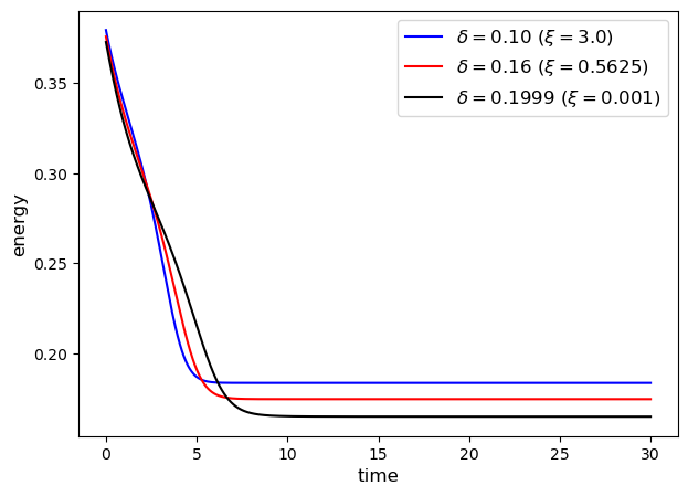
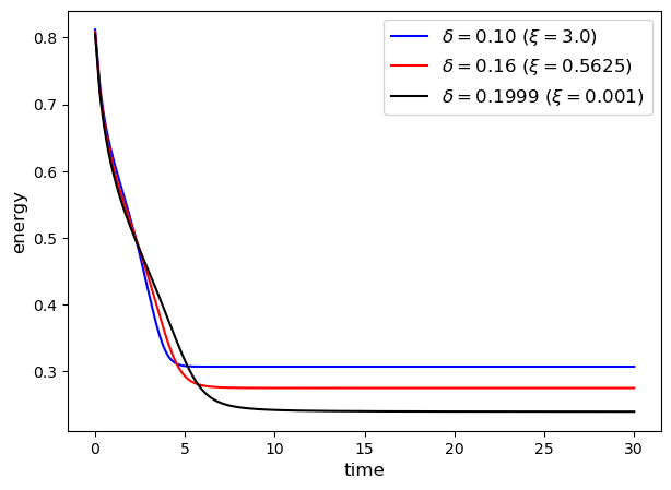
The snapshots of the solutions of the model with the obstacle, regular and logarithmic potentials at different time instances ( $t=10,\ 50$ , and $250$ ) are depicted on Figure 4.3. The solutions are plotted for varying nonlocal interaction parameters $\delta=0.1,0.16,\ 0.1999$ and fixed $\varepsilon=0.1$ , which corresponds to $\xi=3.0,\ 0.5625,\ 0.001$ respectively. The figures at the first and second rows correspond to the solutions of the model with obstacle and regular potentials, whereas the third and fourth rows represent solutions using logarithmic potentials with $\theta_{c}=0.01$ and $\theta_{c}=0.2$ , respectively. In addition, on Figure 4.4, we plot a time evolution of the solution of the model (1.1) with obstacle potential for different values of $\varepsilon=0.2,0.15,$ and $0.1001$ with fixed $\delta=0.2$ , which correspond to $\xi=3.0,\ 1.25,\ 0.002$ , respectively. We observe that the solution develops discontinuity in the interface profile for $\xi\approx 0$ as it approaches the steady-state. This is in agreement with the previously reported results for the obstacle [15] and regular [23] potentials. When using the obstacle potential and $\xi=0$ , the solution exhibits sharp interfaces with only pure phases (Figure 4.3 and Figure 4.4). However, with the regular potential, although a discontinuity develops, it is not a jump discontinuity (the magnitude of the discontinuity being smaller than 2), and a small layer of the solution at the transient phase remains. For the Flory-Huggins potential, the sharpness of the interface is influenced by the parameter $\theta_{c}$ with the sharpness interface achieved for a smaller value of $\theta$ , since for $\theta_{c}\to 0$ the logarithmic potential approaches the obstacle potential.

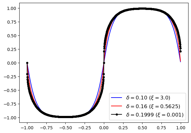
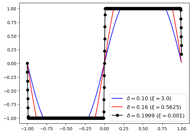
Remark 4.1.

We note that the solution at $x=1$ is excluded for all cases due to the discretization of the periodic boundary conditions.

We also illustrate the sharpness of the interface in two-dimensional setting.

Example 3

We set $\Omega=(-1,1)^{2},$ and set $N=512^{2}$ , $c_{F}=1$ , $\delta=0.0824$ , $\varepsilon^{2}=0.0017$ , corresponding to $\xi=0.0015$ , and $\Delta t=0.005$ . We consider an initial condition given by $u_{0}(x,y)=\sin(\pi x)e^{-|y|}$ and adopt the first order semi-implicit scheme (2.6) to simulate the phase separation until a steady-state. Figure 4.5 shows the evolution of the phase separation at $t=1,3$ , and $50$ for obstacle potential (top), regular potential (middle), and logarithmic potential (bottom) with $\theta_{c}=0.1$ . Additionally, we plot the interface width at $t=50$ (fourth column) for the three potentials with bounds $-1$ and $1$ for obstacle and logarithmic potentials and bounds $-0.99$ and $0.99$ for a regular potential. We observe that, similarly as in 1D case, at a steady-state the sharpest interface appears in the solution with the obstacle potential, whereas the most diffuse interface happens for the case of a regular potential.

4.3. Computational costs

Next, we discuss the computational cost, which is presented in terms of the number of convolution evaluations for each time-stepping scheme. Additionally, we give the $L^{2}$ -errors relative to each computational cost for comprehensive assessment. To compute the errors at a final time $T$ , we perform the numerical simulations with $\Delta t=(T/4)\times 2^{-k},\leavevmode\nobreak\ \leavevmode\nobreak\ k=0,1,2,\dots,13$ and we set the solution obtained by the second order implicit scheme with $\Delta t=(T/4)\times 2^{-15}$ and $TOL=10^{-15}$ in Algorithm 1 as a benchmark solution.

Example 4

We consider $\Omega=(-1,1)^{n},n=1,2,3\leavevmode\nobreak\ c_{F}=2$ , $\delta=\varepsilon=0.15$ , $\theta_{c}=0.5$ , and $T=2$ . We set $N=1024$ , $256^{2}$ , and $80^{3}$ for the 1D, 2D, and 3D cases, respectively. The initial conditions are

$\displaystyle u_{0}(x)$	$\displaystyle=0.1(\sin(\pi x)+\sin(2\pi x))$	$\displaystyle\text{(1D)},$
$\displaystyle u_{0}(x,y)$	$\displaystyle=0.2\sin(\pi x)\sin(\pi y)$	$\displaystyle\text{(2D)},$
$\displaystyle u_{0}(x,y,z)$	$\displaystyle=0.2\sin(\pi x)\sin(\pi y)\sin(\pi z)$	$\displaystyle\text{(3D)}.$

Figures 4.6 and 4.7 display $L^{2}$ -error at the final time with respect to different number of convolution evaluations for obstacle, regular, and logarithmic potentials. We simulate (1.1) for obstacle potential with $n=1,2,3$ , and regular and logarithmic potentials for $n=2$ . We find that the second-order implicit scheme is the most accurate overall, although it requires a larger number of convolution evaluations, as anticipated. Additionally, in scenarios where high precision isn’t essential and a quick approximation is desired, the second-order explicit scheme offers a suitable compromise.

4.4. Dynamics prediction for 3D examples.

We also provide an illustration in a three-dimensional setting. Unless otherwise stated, we consider an obstacle potential case and set $\Omega=(-1,1)^{3}$ , $c_{F}=1.6,\varepsilon=\delta=0.1$ , which corresponds to $\xi=2.4$ , and a time step size $\Delta t=0.005$ .

Example 5

We adopt the second-order explicit scheme to simulate the time evolution of a 3D bubble merging and a star shape up to $T=8$ with mesh size $N=150^{3}.$ The initial conditions of the 3D bubble merging and the star shape are respectively given as

	$\displaystyle u_{0}(x,y,z)=$	$\displaystyle\ \frac{1}{2}\tanh\left(\frac{0.6-\sqrt{(x-0.35)^{2}+y^{2}+z^{2}}}{\sqrt{2}\varepsilon}\right)$
	$\displaystyle+$	$\displaystyle\ \frac{1}{2}\tanh\left(\frac{0.6-\sqrt{(x+0.35)^{2}+y^{2}+z^{2}}}{\sqrt{2}\varepsilon}\right),$
	$\displaystyle u_{0}(x,y,z)=$	$\displaystyle\ \tanh\left(\frac{0.7+0.2\cos(6\eta)-\sqrt{x^{2}+y^{2}+z^{2}}}{\sqrt{2}\varepsilon}\right),$

where,

\eta=\begin{cases}\tan^{-1}\left(\frac{z}{x}\right),\hskip 25.0pt\text{ if }x>0.5,\\ \pi+\tan^{-1}\left(\frac{z}{x}\right),\hskip 5.0pt\text{ otherwise }.\end{cases}

As observed in Figure 4.8, the two balls gradually shrink and merge into one smaller ball, which eventually disappears as expected. For the star shape, the tips of the star move inward, and the gaps between the tips move outward, forming a ball that finally disappears.

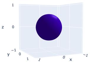
Figure 4.9 presents numerical results for the 2D and 3D simulations with the random initial condition sampled from a uniform distribution, ranging from $-0.95$ to $0.95$ (for 2D) and from $-0.5$ to $0.5$ (for 3D). For the 2D case, we choose $\Omega=(-\pi,\pi)^{2}$ , $c_{F}=1$ , $\varepsilon=0.05,\delta=0.08$ , and $N=512^{2}$ (corresponding to $\xi=0.5625$ ). For the 3D case, we set $\Omega=(-1,1)^{3}$ , $c_{F}=1.6$ , $\varepsilon=0.1,\delta=0.1$ , and $N=60^{3}$ (corresponding to $\xi=2.4$ ).

4.5. Non-isothermal Allen-Cahn model

We demonstrate the applicability of our method to non-isothermal systems, commonly encountered in the solidification of pure materials. Anisotropy is typically inherent in such models and is often represented by imposing nonlinearities on the gradient terms. However, in the nonlocal framework, it can be incorporated through a suitable anisotropic kernel. While we focus on the isotropic model here, our approach can be adapted for nonlocal anisotropic cases, which will be the subject of future work.

More specifically, we consider the following coupled system of equations for the temperature $\theta$ and phase-field variable $u$ :

\displaystyle\begin{dcases}\frac{\partial\theta}{\partial t}=D\Delta\theta+L\frac{\partial u}{\partial t},\\[6.45831pt] \mu\frac{\partial u}{\partial t}+\mathcal{L}u+\partial_{u}\Phi(u,\theta)\ni 0,\end{dcases}

(4.2)

where $D$ , $\mu$ and $L$ are the diffusivity, relaxation time and latent heat coefficients, respectively. Here, $\partial_{u}\Phi(u,\theta)$ is a generalized subdifferential of the double-well potential

\Phi(u,\theta)=F(u)+g(u,\theta),

where $F$ is defined as in (1.4) and $g(u,\theta)$ is an appropriately chosen coupling term. Here, we demonstrate the approach for the obstacle potential, for which $F$ is defined in (1.5) and (1.6) and the coupling term is defined as in [38], see also [15]:

g(u,\theta)=-c_{F}m(\theta)u,\quad\text{with}\quad m(\theta)=\left(\frac{\alpha}{\pi}\right)\tan^{-1}\left(\rho(\theta_{e}-\theta)\right),\quad 0<\alpha<1,

for which it holds that $|m(\theta)|<1/2$ .

We adopt the first-order discretization as outlined in Section 2.1 for the phase-field equation and an implicit Euler time-stepping scheme for the temperature equation. We also use an explicit discretization of the coupling term $m(\theta)$ that allows to fully decouple the problem. Then, the semi-discrete system reads: Find $(\theta^{k},u^{k})$ , $k=1,\dots,K$ such that

\begin{cases}\left(I-\Delta tD\upDelta\right)\theta^{k}=\theta^{k-1}+L(u^{k}-u^{k-1}),\\ u^{k}={P_{[-1,1]}\left(\frac{1}{\mu/\Delta t+\xi}\left(\frac{\mu}{\Delta t}u^{k-1}+\gamma\ast u^{k-1}+c_{F}m(\theta^{k-1})\right)\right).}\end{cases}

First, having $\theta^{k-1}$ using the projection formula, we compute $u^{k}$ . Then, the temperature $\theta^{k}$ is computed from the first equation above. Using the Fourier collocation approach outlined in Section 3 we solve for the temperature in the Fourier space:

\hat{\theta}^{k}_{lm}={\frac{\hat{\theta}^{k-1}_{lm}+L(\hat{u}^{k}_{lm}-\hat{u}^{k-1}_{lm})}{1-D\Delta t\lambda_{mul}}},

(4.3)

where $\lambda_{mul}$ is the multiplier of the Laplacian operator. By applying the inverse Fourier transform, we obtain

\theta^{k}_{ij}=(\mathcal{F}^{-1}_{N}\hat{\theta}^{k})_{ij},

where $(\mathcal{F}^{-1}_{N}\hat{\theta}^{k})_{ij}$ is as defined in (3.2). This is a simple and straightforward approach that allows for an efficient computation of the solution of a coupled non-smooth problem. In the following we provide examples for two- and three-dimensional test cases.

Example 6

We set $\Omega=(-1,1)^{2}$ , $N=512^{2}$ , $c_{F}=1/4$ , $\alpha=0.9$ , $\mu=0.0003$ , $\theta_{e}=1$ , $\rho=10$ , $L=0.5$ , $D=1$ , and adopt the first order semi-implicit scheme to simulate the phase separation up to $T=0.2$ . We choose $\Delta t=0.0001$ , $\delta=0.1,$ and $\varepsilon=0.0251$ , which corresponds to $\xi=0.002$ . The initial conditions are

\displaystyle u_{0}(x,y)=\begin{cases}-1,&-0.9\leq x\leq 0.9,-0.9\leq y\leq 0.9\\ 1,&\text{ otherwise}\end{cases}\text{ and }\theta_{0}\equiv 0.

This example, inspired from an example in [38], see also [15], is an illustration of the solidification of pure materials using nonlocal isothropic model. Here, we have a solid region around the boundaries of the domain and a pool of liquid in the interior. As the time evolves, the solidification that occurs from the walls propagates inward until all liquid solidifies. As illustrated in Figure 4.10, this corresponds to the liquid region (marked in blue) in the snapshot of the phase-field variable to gradually shrink over time and eventually disappears.

Lastly, we demonstrate the performance of the model in three-dimensional case using deterministic and random initial conditions for the phase-field variable and constant temperature.

Example 7

We set $\Omega=(-1,1)^{3}$ , $N=100^{3}$ , $\Delta t=0.0001$ and adopt the same parameter settings as in the previous example, along with similar initial conditions:

\displaystyle u_{0}({\bf{x}})=\begin{cases}-1,&-0.9\leq{\bf{x}}\leq 0.9,\ {\bf{x}}\in\mathbb{R}^{3},\\ 1,&\text{ otherwise}\end{cases}\quad\text{ and }\theta_{0}\equiv 0.

The corresponding snapshots of the phase-field variable are presented on Figure 4.11 (top row). We can observe a similar behavior in the solution as seen in the two-dimensional case. Next, we consider a random initial condition for the phase-field variable $u$ , taken to be a Gaussian random field with mean zero and Gaussian covariance kernel. We consider the same settings as before, apart from $\mu=0.0005$ , $T=0.003$ and chose $\delta=0.1,$ and $\varepsilon=0.08$ , which corresponds to $\xi=2.31$ . On Figure 4.11 we present the snapshots of the time evolution for the phase-field variable.

5. Conclusion

In this work, we present a comprehensive approach to discretizing the nonlocal Allen-Cahn equation, considering both temporal and spatial dimensions. We design first and second-order energy-stable temporal discretizations, complemented by efficient spatial discretization using the Fourier collocation method based on FFT, resulting in a fully scalable and efficient method. Future research could enhance and broaden this approach by exploring its application to more complex equations like Cahn-Hilliard or non-isothermal systems, and more complex boundary conditions or geometries. Additionally, investigating parallelization techniques for scalability in high-performance computing environments would be valuable.

References

[1] Ainsworth, M., and Glusa, C. Aspects of an adaptive finite element method for the fractional laplacian: A priori and a posteriori error estimates, efficient implementation and multigrid solver. Computer Methods in Applied Mechanics and Engineering 327 (2017), 4–35. Advances in Computational Mechanics and Scientific Computation—the Cutting Edge.
[2] Alali, B., and Albin, N. Fourier spectral methods for nonlocal models. Journal of Peridynamics and Nonlocal Modeling 2 (2020), 317–335.
[3] Alali, B., and Albin, N. Fourier multipliers for nonlocal laplace operators. Applicable Analysis 100, 12 (2021), 2526–2546.
[4] Bates, P. W. On some nonlocal evolution equations arising in materials science. Nonlinear dynamics and evolution equations 48 (2006), 13–52.
[5] Bates, P. W., Brown, S., and Han, J. Numerical analysis for a nonlocal Allen-Cahn equation. Int. J. Numer. Anal. Model 6, 1 (2009), 33–49.
[6] Bates, P. W., and Chmaj, A. An Integrodifferential Model for Phase Transitions: Stationary Solutions in Higher Space Dimensions. Journal of Statistical Physics 95, 5 (1999), 1119–1139.
[7] Bates, P. W., Fife, P. C., Ren, X., and Wang, X. Traveling waves in a convolution model for phase transitions. Archive for Rational Mechanics and Analysis 138, 2 (1997), 105–136.
[8] Bauschke, H. H., and Combettes, P. L. Convex Analysis and Monotone Operator Theory in Hilbert Spaces, 2nd ed. Springer Publishing Company, Incorporated, 2017.
[9] Beneš, M., Chalupecký, V., and Mikula, K. Geometrical image segmentation by the allen–cahn equation. Applied Numerical Mathematics 51, 2 (2004), 187–205.
[10] Blank, L., Butz, M., Garcke, H., Sarbu, L., and Styles, V. Allen-Cahn and Cahn-Hilliard Variational Inequalities Solved with Optimization Techniques. Springer Basel, Basel, 2012, pp. 21–35.
[11] Blank, L., Butz, M., and Garcke, H. Solving the Cahn-Hilliard variational inequality with a semi-smooth Newton method. ESAIM: COCV 17, 4 (2011), 931–954.
[12] Borthagaray, J. P., Nochetto, R. H., and Salgado, A. J. Weighted Sobolev regularity and rate of approximation of the obstacle problem for the integral fractional Laplacian. Mathematical Models and Methods in Applied Sciences 29, 14 (2019), 2679–2717.
[13] Bosch, J., Stoll, M., and Benner, P. Fast solution of Cahn–Hilliard variational inequalities using implicit time discretization and finite elements. Journal of Computational Physics 262 (2014), 38 – 57.
[14] Boyd, S., and Parikh, N. Proximal algorithms. Foundations and Trends in optimization 1, 3 (2013), 123–231.
[15] Burkovska, O. Non-isothermal nonlocal phase-field models with a double-obstacle potential, 2023.
[16] Burkovska, O., and Gunzburger, M. Regularity analyses and approximation of nonlocal variational equality and inequality problems. Journal of Mathematical Analysis and Applications 478, 2 (2019), 1027–1048.
[17] Burkovska, O., and Gunzburger, M. On a nonlocal Cahn–Hilliard model permitting sharp interfaces. Mathematical Models and Methods in Applied Sciences 31, 09 (2021), 1749–1786.
[18] Chen, X. Existence, uniqueness, and asymptotic stability of traveling waves in nonlocal evolution equations. Adv. Differential Equations 2 (1997), 125–160.
[19] D’Elia, M., Du, Q., Glusa, C., Gunzburger, M. D., Tian, X., and Zhou, Z. Numerical methods for nonlocal and fractional models. To appear in Acta Numerica (2021).
[20] Du, Q., and Feng, X. Chapter 5 - the phase field method for geometric moving interfaces and their numerical approximations. In Geometric Partial Differential Equations - Part I, A. Bonito and R. H. Nochetto, Eds., vol. 21 of Handbook of Numerical Analysis. Elsevier, 2020, pp. 425–508.
[21] Du, Q., Ju, L., Li, X., and Qiao, Z. Stabilized linear semi-implicit schemes for the nonlocal Cahn–Hilliard equation. Journal of Computational Physics 363 (2018), 39–54.
[22] Du, Q., Ju, L., Li, X., and Qiao, Z. Maximum Principle Preserving Exponential Time Differencing Schemes for the Nonlocal Allen–Cahn Equation. SIAM Journal on Numerical Analysis 57, 2 (2019), 875–898.
[23] Du, Q., and Yang, J. Asymptotically Compatible Fourier Spectral Approximations of Nonlocal Allen–Cahn Equations. SIAM Journal on Numerical Analysis 54, 3 (2016), 1899–1919.
[24] Du, Q., and Yang, J. Fast and accurate implementation of fourier spectral approximations of nonlocal diffusion operators and its applications. Journal of Computational Physics 332 (2017), 118–134.
[25] Fife, P. C. Travelling waves for a nonlocal double-obstacle problem. European Journal of Applied Mathematics 8, 6 (1997), 581–594.
[26] Geng, Y., Burkovska, O., Gunzburger, M., Ju, L., and Zhang, G. An end-to-end deep learning method for solving nonlocal Allen-Cahn and Cahn-Hilliard phase-field models. Preprint (2024).
[27] Geng, Y., Teng, Y., Wang, Z., and Ju, L. A deep learning method for the dynamics of classic and conservative allen-cahn equations based on fully-discrete operators. Journal of Computational Physics 496 (2024), 112589.
[28] Guan, Q., and Gunzburger, M. Analysis and approximation of a nonlocal obstacle problem. Journal of Computational and Applied Mathematics 313 (2017), 102–118.
[29] Guan, Q., Gunzburger, M., Webster, C. G., and Zhang, G. Reduced basis methods for nonlocal diffusion problems with random input data. Computer Methods in Applied Mechanics and Engineering 317 (2017), 746–770.
[30] Guan, Z., Lowengrub, J., and Wang, C. Convergence analysis for second-order accurate schemes for the periodic nonlocal Allen-Cahn and Cahn-Hilliard equations. Mathematical Methods in the Applied Sciences 40, 18 (2017), 6836–6863.
[31] Guan, Z., Lowengrub, J. S., Wang, C., and Wise, S. M. Second order convex splitting schemes for periodic nonlocal Cahn–Hilliard and Allen–Cahn equations. Journal of Computational Physics 277 (2014), 48–71.
[32] Gwiazda, P., Skrzeczkowski, J., and Trussardi, L. On the rate of convergence of Yosida approximation for the nonlocal Cahn–Hilliard equation. IMA Journal of Numerical Analysis (2024), 1–19.
[33] Hartley, T., and Wanner, T. A semi-implicit spectral method for stochastic nonlocal phase-field models. Discrete and Continuous Dynamical Systems 25, 2 (2009), 399–429.
[34] Hintermüller, M., Ito, K., and Kunisch, K. The primal-dual active set strategy as a semismooth Newton method. SIAM Journal on Optimization 13, 3 (2002), 865–888.
[35] Hintermüller, M., Hinze, M., and Kahle, C. An adaptive finite element Moreau–Yosida-based solver for a coupled Cahn–Hilliard/Navier–Stokes system. Journal of Computational Physics 235 (2013), 810–827.
[36] Hintermüller, M., Hinze, M., and Tber, M. H. An adaptive finite-element Moreau–Yosida-based solver for a non-smooth Cahn–Hilliard problem. Optimization Methods and Software 26, 4-5 (2011), 777–811.
[37] Jafarzadeh, S., Larios, A., and Bobaru, F. Efficient solutions for nonlocal diffusion problems via boundary-adapted spectral methods. Journal of Peridynamics and Nonlocal Modeling (2020), 1–26.
[38] Kobayashi, R. Modeling and numerical simulations of dendritic crystal growth. Physica D: Nonlinear Phenomena 63, 3 (1993), 410 – 423.
[39] Li, Z., Wang, H., and Yang, D. A space–time fractional phase-field model with tunable sharpness and decay behavior and its efficient numerical simulation. Journal of Computational Physics 347 (2017), 20–38.
[40] Luo, X., and Bertozzi, A. L. Convergence of the graph allen–cahn scheme. Journal of Statistical Physics 167 (2017), 934–958.
[41] Miranville, A. The Cahn-Hilliard equation and some of its variants. AIMS Mathematics 2, 3 (2017), 479–544.
[42] Mustapha, I., Alali, B., and Albin, N. Regularity of solutions for nonlocal diffusion equations on periodic distributions. Journal of Integral Equations and Applications 35, 1 (2023), 81–104.
[43] Shen, J., Tang, T., and Wang, L.-L. Spectral methods: algorithms, analysis and applications, vol. 41. Springer Science & Business Media, 2011.
[44] Tian, X., and Du, Q. Asymptotically compatible schemes and applications to robust discretization of nonlocal models. SIAM Journal on Numerical Analysis 52, 4 (2014), 1641–1665.
[45] Tian, X., and Du, Q. Asymptotically compatible schemes for robust discretization of parametrized problems with applications to nonlocal models. SIAM Review 62, 1 (2020), 199–227.
[46] Trefethen, L. N. Spectral methods in MATLAB. SIAM, 2000.
[47] Wheeler, A., Murray, B., and Schaefer, R. Computation of dendrites using a phase field model. Physica D: Nonlinear Phenomena 66, 1 (1993), 243–262.
[48] Wituła, R., and Słota, D. Cardano’s formula, square roots, chebyshev polynomials and radicals. Journal of Mathematical Analysis and Applications 363, 2 (2010), 639–647.