An efficient distributed scheduling algorithm for relay-assisted mmWave backhaul networks

To elaborate the handshaking process, an example is provided in Figure 1. A small backhaul network with a tree topology is shown in the lower part of Figure 1, where BS 1 is the macro-cell BS, and BS 2-5 are all small-cell BSs.

It is noticed that some logical links between BSs are multi-hop relay paths. If control messages are sent through the multi-hop logical links, the delay of these control information will be too long. To address this issue, each BS is equipped with a communication module working at a lower frequency band (e.g., sub-6 Ghz band), which uses an omni-directional antenna. That communication module takes responsibility of transmitting and receiving control messages in the first two control slots of each subframe. To avoid the collision of the control messages between a BS and its child BSs, each control slot is further partitioned into $n_{sub}$ sub-slots, and each child BS is assigned a unique sub-slot to exchange control messages. The assignment of sub-slots between a BS and its child BSs happens in the initial configuration phase when the relay-assisted backhaul network is constructed. During the initial configuration phase, a child BS is associated with its parent BS to form the backhaul logical link.

As we can see in Figure 1, at the first slot of each subframe, each small-cell BS calculates its local schedule based on the traffic demand information, which will be explained in detail later. The calculated local schedule and updated queue and traffic demand information of a small-cell BS will be sent immediately to its parent BS. Note that, since there is no parent BS of the macro-cell BS, it will skip this step.

After a BS receives the control messages from its child BSs, before it starts the calculation of a final valid schedule for a specific future subframe, it checks whether the final valid schedule from its parent BS for the same future subframe has been received or not. If it has not been received, the BS will not schedule transmissions in that future subframe, because it does not know which slots are assigned to the logical link between itself and its parent BS. Any transmission from the BS may potentially conflict with the transmission from its parent BS. On the other hand, if the interested final valid schedule from the parent BS has been received, the BS will starts the calculation of its final valid schedule.

As shown in the example, each BS will start its scheduling in a specific subframe according to its height in the tree topology. If the topology has a depth of $H$, which is the height of the macro-cell BS and each small-cell BS $B_{i}$’s height is denoted as $h_{i}$, the macro-cell BS will start its scheduling in subframe 1, while small-cell BS $B_{i}$ will start its scheduling in subframe ($H-h_{i}+1$). Note that, because the schedule of leaf BSs is determined by their parent BSs, they do not calculate their final valid schedule.

Moreover, in the first scheduling subframe, each non-leaf BS will calculate its schedule of the next several subframes in advance (i.e., from subframe $H-h_{i}+1$ to subframe $H$), because when a child BS calculates its final valid schedule of a subframe, it has to know its parent BS’s final valid schedule of the same subframe in advance; however, the schedule needs time to propagate to its child BSs. After the first scheduling subframe, each BS only needs to calculate the final valid schedule of the next unscheduled subframe. As depicted in Figure 1, the initialization phase lasts $H-1$ subframe, and after that, the stable phase starts.

The purpose of calculating the local schedule on a small-cell BS $B_{i}$ is to obtain the “desired” number of slots that $B_{i}$ wants its parent BS $B_{i}^{p}$ to assign for the data transmission on the logical link $L_{i}$ between $B_{i}$ and $B_{i}^{p}$. As a “desired” local optimal, it is calculated based on the local traffic demand information rather than the queue information.

Traffic demand information is an upper layer (i.e., application) statistics which is not typically used in the scheduling algorithm (i.e., MAC layer) in wireless ad hoc or mesh networks. However, in cellular networks starting from the 4G-LTE systems, the Quality-of-Service (QoS) has become a key performance metric. QoS related policies such as traffic classification and prioritization have already been installed in BSs. Application or service data rate of each user accessing to a BS, as a crucial QoS parameter, is constantly collected by the BS. In the 5G system, as a wider range of applications are going to be supported, even finer-grained management of QoS is expected to be implemented, which means more accurate traffic demand information is likely available at each BS [32]. In fact, the local schedule aims to provide a “desired” resource allocation requirement to the parent BS, the amount of which is usually much larger than the amount of resource that the parent BS can offer in a backhaul network with the heavy traffic load. From this point of view, a small estimation error on the traffic demand of each BS is acceptable. From the discussion in the above section 5.1, we know that each BS keeps updating its traffic demand information to its parent BS; thus, after a certain amount of time, BS $B_{i}$ can obtain the accurate total traffic demand $D_{j}$ from its child BS $B_{j}\in\mathcal{B}_{i}^{c}$, where $\mathcal{B}_{i}^{c}$ is the set of child BSs of $B_{i}$. Note that, first, the traffic demand $D_{j}$ of $B_{j}$ is in fact the aggregated traffic demand of all small-cell BSs in the sub-tree rooted at $B_{j}$; second, as the proposed distributed algorithm schedules both uplink and downlink traffic, the traffic demand information contains both the downlink traffic demand and the uplink traffic demand information.

The local schedule of $B_{i}$ indicates the number of slots assigned for the data transmissions (both uplink and downlink) on all physical links attached to $B_{i}$. We denote the number of slots assigned to the attached physical link within the logical link $L_{j}$ as $n_{j}$. Note that, the demand may exceed the maximum throughput capacity of a BS; therefore, we use a local continuous scale variable $S_{i}$ to indicate the fraction of traffic demand of each child BS actually being served at $B_{i}$ in one subframe. From this perspective, our proposed distributed scheduling algorithm addresses the local fairness through proportionally schedule the data traffic according to the amount of the traffic demand of each child BS.

Based on the above system setting, we can formulate a mixed integer programming problem to address the calculation of the local scheduling on $B_{i}$, in which the local scale variable $S_{i}$ is to be maximized. In Equation 1, continuous variable $S_{i}$ is the optimization objective, and integer variables $\{n_{j}|\ B_{j}\in B_{i}\bigcup\mathcal{B}_{i}^{c}\}$ are auxiliary variables.

$$\begin{split}\max\quad&S_{i}\\ \mathrm{s.t.}\quad&n_{i}\cdot r_{ii}\geq S_{i}\cdot\sum_{B_{j}\in B_{i}\bigcup\mathcal{B}_{i}^{c}}{D_{j}}\\ &0\leq S_{i}\leq 1\\ &n_{j}\cdot r_{ji}\geq S_{i}\cdot D_{j},\ \forall\ B_{j}\in\mathcal{B}_{i}^{c}\\ &\frac{1}{P_{ji}}\leq\frac{n_{j}}{P_{ji}}\leq n_{d},\ \mathrm{if}\ D_{j}>0,\ \forall\ B_{j}\in B_{i}\bigcup\mathcal{B}_{i}^{c}\\ &{n_{j}}=0,\ \mathrm{if}\ D_{j}=0,\ \forall\ B_{j}\in B_{i}\bigcup\mathcal{B}_{i}^{c}\\ &\lceil\frac{n_{j}}{P_{ji}}\rceil+I_{jk}\cdot{\lceil\frac{n_{k}}{P_{ki}}\rceil}\leq n_{d},\ \forall\ B_{j},B_{k}\in B_{i}\bigcup\mathcal{B}_{i}^{c}\\ &\sum_{B_{j}\in B_{i}\bigcup\mathcal{B}_{i}^{c}}{n_{j}}\leq n_{d}\cdot N_{i}^{R}\end{split}$$

(1)

As the distributed scheduling algorithm is expected to operate in the real relay-assisted mmWave backhaul system, in which every physical link has a length in the order of 200 m. Due to the use of high-gain highly-directional antennas, the data transmissions on these LoS physical links are likely to be able to use the highest level of modulation (e.g., 256 QAM) allowed in the system. Therefore, the physical link data rate is the same, and we denote the unified physical link data rate as $r$. Since the portion $P_{ji}$ of the transmission on the physical link within the logical link $L_{j}$ attached to $B_{i}$ is either 1 (i.e., single-hop) or 0.5 (i.e., multi-hop), we define a new integer parameter $\alpha_{ji}=\frac{1}{P_{ji}}$, whose value is either 1 or 2. Therefore, we can update the above mixed integer programming problem into a mixed integer linear programming problem.

$$\begin{split}\max\quad&S_{i}\\ \mathrm{s.t.}\quad&n_{i}\cdot r\geq S_{i}\cdot\sum_{B_{j}\in B_{i}\bigcup\mathcal{B}_{i}^{c}}{D_{j}}\\ &0\leq S_{i}\leq 1\\ &n_{j}\cdot r\geq S_{i}\cdot D_{j},\ \forall\ B_{j}\in\mathcal{B}_{i}^{c}\\ &\alpha_{ji}\leq\alpha_{ji}\cdot{n_{j}}\leq n_{d},\ \mathrm{if}\ D_{j}>0,\ \forall\ B_{j}\in B_{i}\bigcup\mathcal{B}_{i}^{c}\\ &{n_{j}}=0,\ \mathrm{if}\ D_{j}=0,\ \forall\ B_{j}\in B_{i}\bigcup\mathcal{B}_{i}^{c}\\ &\alpha_{ji}\cdot{n_{j}}+I_{jk}\cdot{\alpha_{ki}\cdot{n_{k}}}\leq n_{d},\ \forall\ B_{j},B_{k}\in B_{i}\bigcup\mathcal{B}_{i}^{c}\\ &\sum_{B_{j}\in B_{i}\bigcup\mathcal{B}_{i}^{c}}{n_{j}}\leq n_{d}\cdot N_{i}^{R}\end{split}$$

(2)

Since in the real system, $\mathcal{B}_{i}^{c}$ is a small set, $n_{d}$ is a pre-set small integer, the known interference relationship matrix $\{I_{jk}\}$ is sparse, the computation time for solving this mixed integer linear programming problem is very short. After solving the problem, the maximum $S_{i}$ is found, and correspondingly, we can calculate the minimum number of time slots $\widehat{n_{i}}$ to support the maximum achievable traffic demand for the physical link attached to $B_{i}$ within $L_{i}$. $\widehat{n_{i}}$ is the key parameter of the local schedule, which will be transmitted to $B_{i}$’s parent BS, as it indicates the maximum time slots that the parent BS shall allocate to the physical link within $L_{i}$. The parent BS could allocate more time slots to $L_{i}$; however, the extra traffic cannot be absorbed timely by $B_{i}$, as the total traffic on $L_{i}$ exceeds the maximum achievable traffic demand of $B_{i}$.

In the real deployment of the distributed algorithm, since the traffic demand of each small-cell BS may be fluctuating within a small range in most of time or it changes gradually in a slow speed, the calculation of local schedule may fall into the trouble of tracking the demand change too sensitively, such that the final valid schedule may be changing too frequently as well. To address this issue, we modify the message exchange of local schedule that the BS $B_{i}$ only updates the value of $\widehat{n_{i}}$ to its parent BS when significant changes of $\widehat{n_{i}}$ happens. Specifically, $B_{i}$ keeps recording the temporary $\widehat{n_{i}}$ value calculated in each subframe, and it applies a sliding window on the sequence of $\widehat{n_{i}}$ values to get the time-averaged value $\bar{\widehat{n_{i}}}$. When the difference between the current reporting $\widehat{n_{i}}$ value and the time-averaged value $\bar{\widehat{n_{i}}}$ is larger than a threshold of $T$ percentage, the reporting $\widehat{n_{i}}$ value is updated to $\bar{\widehat{n_{i}}}$; otherwise the reporting value does not change. In our simulations, we choose a relatively large threshold (i.e., 50%), so that in a small backhaul network (e.g., 20 BSs), few small-cell BSs will experience sharp traffic demand change simultaneously.

After a BS receives the queue, traffic and local schedule information from its child BSs, it will determine its schedule of a future subframe based on its height in the topology, as mentioned in the above section on hand-shaking. Different from the calculation of local schedule, the valid schedule is determined using not only the traffic demand information, but also the queue and local schedule information.

To realize the distributed algorithm, a non-leaf small-cell BS $B_{i}$ has to maintain queues to store downlink and uplink packets, whose destinations are not $B_{i}$. We use $\mathcal{B}_{i}$ to denote the set of BSs located in the sub-tree rooted at $B_{i}$. For each small-cell BS $B_{k}\in\mathcal{B}_{i}$, $B_{i}$ maintains a downlink queue and a uplink queue for it, which temporarily store all packets with the same destination BS as $B_{k}$ and all packets to be routed to the macro-cell BS $M$ with the same source BS as $B_{k}$, respectively. At the beginning of a subframe on $B_{i}$, the total number of packets to $B_{k}$ in the corresponding downlink queue is $q_{i,k}^{D}$; while the total number of packets from $B_{k}$ in the corresponding uplink queue is $q_{i,k}^{U}$.

However, the set of queue lengths actually used in the final valid schedule calculation are related to the routing, because we need to know the exact total number of uplink and downlink packets that wait to be transmitted on each logical link $L_{j}$ between $B_{i}$ and $B_{i}$’s each child BS $B_{j}$. Therefore, at BS $B_{i}$, the total number of downlink packets waiting to be transmitted on $L_{j}$ is denoted as $Q_{i,j}^{D}$. Meanwhile, the uplink packets waiting to be transmitted on $L_{j}$ are stored in the uplink queues at $B_{j}$, and the total number of them is denoted as $Q_{j}^{U}$.

$$\begin{split}Q_{i,j}^{D}=\sum_{B_{k}\in\mathcal{B}_{j}}{q_{i,k}^{D}}\\ Q_{j}^{U}=\sum_{B_{k}\in\mathcal{B}_{j}}{q_{j,k}^{U}}\\ \end{split}$$

(3)

Based on Equation 3, the total number of uplink and downlink packet waiting to be transmitted on $L_{j}$ is $Q_{j}$, and

$$Q_{j}=Q_{i,j}^{D}+Q_{j}^{U}$$

(4)

As mentioned in the “handshaking” procedure, at the first time slot of each subframe, the child BS $B_{j}$ transmits the uplink queue information $Q_{j}^{U}$ to its parent BS $B_{i}$, so that $Q_{j}$ can be updated timely before the calculation of final schedule begins. Note that the queue maintenance on the macro-cell BS $M$ and the leaf small-cell BS is similar to that on the small-cell BS, except that $M$ does not have uplink queues and leaf small-cell BSs do not have downlink queues. There is no parent BS of the macro-cell BS and no child BS of the leaf small-cell BSs. The process of generating the valid schedule of a BS varies according to the type of that BS.

In this section, simulations are conducted to evaluate the throughput performance of the proposed distributed scheduling algorithm. In the simulations, the physical link data rate is set to 13.3 Gbps as discussed in section 5.2. There are in total 24 slots within a subframe which lasts for 0.1 ms, and the first two slots of each subframe is reserved to implement the operation of handshaking procedure described in section 5.1. The rest 22 slots are data slots which can be used to transmit both uplink and downlink data traffic. All backhaul topologies used in the simulations are generated using a spanning-tree algorithm introduced in the section 4.3 of [33].

Figure 2 shows the throughput performance of the distributed algorithm in different network settings (i.e., the interference condition and the number of radio chains available on each BS) under different traffic loads from 0.67 Gbps to 3.33 Gbps at each small-cell BS. Note that, all the simulated throughput values are averaged across 50 sets of individual simulations in each scenario. In each simulation, the ratio between the uplink and downlink input traffic demand of a small-cell BS is 1:2, and each small-cell BS has the same traffic demand. Each individual simulation runs for 1000 subframes. In Figure 2, we can see that the throughput performance of the “MI-ER” scenario (i.e., interference-minimal and enough radio chains available) is much better than that of the “LI-LR (2)” scenario (i.e., interference exists between a few pairs of logical links, and 2 radio chains on the macro-cell BS while 1 radio chain on each small-cell BS). This is because the maximum traffic demand achievable of each small-cell BS in the “MI-ER” case is much higher than that of the “LI-LR (2)” case. In fact, using the updated link capacity and $\{p_{i}^{f}\}$ values, we can get the updated maximum traffic demand of each small-cell BS in the “MI-ER” case as 1.64 Gbps in average; while the value of the “LI-LR (2)” case is 0.94 Gbps. As Figure 2 shows, the maximum throughput values in the simulation are close to the calculated maximum traffic demand values in both scenarios, which means the distributed algorithm can schedule the transmissions efficiently in the mmWave backhaul networks.

It is noticed that the determination of the final valid schedule on BSs strictly follows the idea of scheduling the backhaul traffic proportionally according to the queue length of each flow bounded by the traffic demand of each corresponding small-cell BS. Although it addresses the fairness issue, the utilization of the network resource could be low when there exist several bottleneck routes in the backhaul network. On those bottleneck routes, if the aggregated traffic demand is much larger than the network capacity of the routes, it leads to very small values of the optimized scaling variable $S$. As the local $S_{M}$ value is applied to all routes in the network at the macro-cell BS, a very small $S_{M}$ will limit the amount of traffic transferred on those non-bottleneck routes, where plenty unused network resource may exist.

To improve the low network resource utilization and increase the network aggregated throughput, we add a step in the determination of the final valid schedule after the optimization of $S_{M}$ at the macro-cell BS. In this new step, the optimized $\widehat{S_{M}}$ is used to bound smallest amount of traffic demand of each small-cell BS that has to be serve in a subframe. In Equation 7, we can see that the new optimization objective is to maximize the number of data slots used in one subframe.

$$\begin{split}\max\quad&\sum_{B_{j}\in\mathcal{B}_{M}^{c}}{n_{j}}\\ \mathrm{s.t.}\quad&n_{j}\cdot r\geq\widehat{S_{M}}\cdot\min{\{Q_{j},D_{j}\}},\ \forall\ B_{j}\in\mathcal{B}_{M}^{c}\\ &1\leq{n_{j}}\leq\widehat{n_{j}},\ \mathrm{if}\ Q_{j}>0,\ \forall\ B_{j}\in\mathcal{B}_{M}^{c}\\ &n_{j}=0,\ \mathrm{if}\ Q_{j}=0,\ \forall\ B_{j}\in\mathcal{B}_{M}^{c}\\ &\alpha_{j}\cdot{n_{j}}+I_{jk}\cdot{\alpha_{k}\cdot{n_{k}}}\leq n_{d},\ \forall\ B_{j},B_{k}\in\mathcal{B}_{M}^{c}\\ &\sum_{B_{j}\in\mathcal{B}_{M}^{c}}{n_{j}}\leq n_{d}\cdot N_{M}^{R}\end{split}$$

(7)

We conduct simulations to compare the aggregated throughput achieved by using the modified distributed scheduling algorithm and the maximized aggregated traffic demand at the macro-cell BS that can be supported by the backhaul network, which is obtained in [19]. In our distributed scheduling simulations, the traffic demand of each small-cell BS is set as 3.33 Gbps, and the aggregated traffic demand surpasses the network capacity. As we can see in Figure 3, in both MIER and LILR(2) scenarios, the aggregated throughput achieved using the modified algorithm is close to the maximized traffic demand that can be supported by the backhaul network. It shows that our proposed algorithm can schedule the backhaul traffic efficiently.

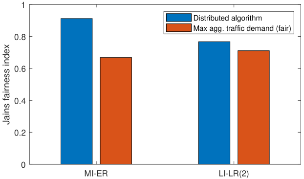
Moreover, as the input traffic demand is the same on each small-cell BS, we also calculate the Jain’s fairness index of the set of throughput values of all small-cell BSs obtained in the distributed scheduling simulation. Figure 4 shows that our algorithm can provide better fairness than the case in the theoretical analysis in [19] can. Because in [19], the optimization does not address the fairness issue in the allocation of the extra to be supported traffic demand among small-cell BSs. In the solution to the optimization problem obtained in the theoretical analysis, usually the extra traffic demand is allocated to only a few BSs, which leads to an unfair situation. In contrary, using our distributed algorithm, the extra traffic demand is allocated locally fairly due to the procedure of determining final valid schedule at small-cell BSs.

In the practical backhaul system, the traffic demand of each small-cell BS may be fluctuating within a small range in most of the time or it changes gradually with a slow speed; therefore, during a relatively long period of time, only a few BSs are likely to experience sharp traffic demand change. In this simulation, we aim to explore the feature of our proposed distributed scheduling algorithm on tracking the dynamic traffic demand (with sharp demand change) of a small-cell BS in the backhaul network. The topology used in the simulation is shown in Figure 5, where the targeting BS is marked as $B^{*}$.

In the simulation, the traffic demand of all small-cell BSs is initialized as 0.67 Gbps for downlink and 0.33 Gbps for uplink. When time arrives at the 250-th subframe, the downlink traffic demand of $B^{*}$ is doubled to 1.34 Gbps; while its uplink traffic demand is unchanged until the 400-th subframe. Starting from the 400-th subframe, the uplink traffic demand of $B^{*}$ is doubled. The downlink and uplink traffic demands of $B^{*}$ are set back to their initial values at the 600-th and 750-th subframe, respectively.

Figure 6 shows the dynamic throughput within each subframe of $B^{*}$. From the figure, we can see that the proposed distributed scheduling algorithm can track the sharp traffic demand change quickly and accurately. In fact, when the downlink traffic demand doubles, it takes 8 subframes for the instantaneous downlink throughput to jump to the new stage; while it takes 13 subframes for the instantaneous downlink throughput to drop back to the old stage, after the downlink traffic demand sets back to the original value. Correspondingly, the two values of number of subframes used to track the uplink traffic demand changes are 4 and 8. The selected BS has a height of 4 in the topology. In the downlink traffic demand change case, the traffic demand change has to first propagate to the macro-cell BS to increase the “desired” time slots for the logical links in the route. After that, more packets can be transferred to the targeting BS. However, in the uplink case, the increased uplink traffic flows together with the “traffic increasing” message to the macro-cell BS, which is a one-way trip intuitively. When the traffic demand drops, it takes a bit longer time for the throughput to drop, because the packets from the heavy traffic queued in the intermediate BSs need time to be absorbed by $B^{*}$.

References

- [1] B. Rong, M. Dianati, L. Zhou, G. K. Karagiannidis, and C. Wang, “5g mmwave small cell networks: architecture, self-organization, and management,” IEEE Wireless Communications, vol. 25, no. 4, pp. 8–9, 2018.
- [2] C. Liu, M. Li, S. V. Hanly, P. Whiting, and I. B. Collings, “Millimeter-wave small cells: Base station discovery, beam alignment, and system design challenges,” IEEE Wireless Communications, vol. 25, no. 4, pp. 40–46, 2018.
- [3] W. Feng, Y. Li, D. Jin, L. Su, and S. Chen, “Millimetre-wave backhaul for 5g networks: Challenges and solutions,” Sensors, vol. 16, no. 6, p. 892, 2016.
- [4] M. Jaber, M. A. Imran, R. Tafazolli, and A. Tukmanov, “5G backhaul challenges and emerging research directions: A survey,” IEEE Access, vol. 4, pp. 1743–1766, 2016.
- [5] R. Taori and A. Sridharan, “Point-to-multipoint in-band mmwave backhaul for 5g networks,” IEEE Communications Magazine, vol. 53, no. 1, pp. 195–201, 2015.
- [6] M. Shariat, M. Dianati, K. Seppänen, T. Suihko, J. Putkonen, and V. Frascolla, “Enabling wireless backhauling for next generation mmwave networks,” in 2015 European conference on networks and communications (EuCNC), pp. 164–168, IEEE, 2015.
- [7] M. Polese, M. Giordani, T. Zugno, A. Roy, S. Goyal, D. Castor, and M. Zorzi, “Integrated access and backhaul in 5g mmwave networks: Potential and challenges,” IEEE Communications Magazine, vol. 58, no. 3, pp. 62–68, 2020.
- [8] C. Saha, M. Afshang, and H. S. Dhillon, “Integrated mmwave access and backhaul in 5g: Bandwidth partitioning and downlink analysis,” in 2018 IEEE International Conference on Communications (ICC), pp. 1–6, IEEE, 2018.
- [9] C. Madapatha, B. Makki, C. Fang, O. Teyeb, E. Dahlman, M.-S. Alouini, and T. Svensson, “On integrated access and backhaul networks: Current status and potentials,” IEEE Open Journal of the Communications Society, vol. 1, pp. 1374–1389, 2020.
- [10] Y. Liu and D. M. Blough, “Analysis of blockage effects on roadside relay-assisted mmwave backhaul networks,” in ICC 2019-2019 IEEE International Conference on Communications (ICC), pp. 1–7, IEEE, 2019.
- [11] M. Gerasimenko, D. Moltchanov, M. Gapeyenko, S. Andreev, and Y. Koucheryavy, “Capacity of multiconnectivity mmwave systems with dynamic blockage and directional antennas,” IEEE Transactions on Vehicular Technology, vol. 68, no. 4, pp. 3534–3549, 2019.
- [12] Q. Hu and D. M. Blough, “Relay selection and scheduling for millimeter wave backhaul in urban environments,” in 2017 IEEE 14th International Conference on Mobile Ad Hoc and Sensor Systems (MASS), pp. 206–214, IEEE, 2017.
- [13] Q. Hu and D. M. Blough, “Optimizing millimeter-wave backhaul networks in roadside environments,” in Communication (ICC), 2018 IEEE International Conference on, IEEE, 2018.
- [14] Q. Hu and D. M. Blough, “On the feasibility of high throughput mmwave backhaul networks in urban areas,” in 2020 International Conference on Computing, Networking and Communications (ICNC), pp. 572–578, IEEE, 2020.
- [15] Y. Yan, Q. Hu, and D. M. Blough, “Load-balanced routing for hybrid fiber/wireless backhaul networks,” in 2021 IEEE Global Communications Conference (GLOBECOM), pp. 1–6, IEEE, 2021.
- [16] Y. Liu, Q. Hu, and D. M. Blough, “Joint link-level and network-level reconfiguration for mmwave backhaul survivability in urban environments,” in Proceedings of the 22nd International ACM Conference on Modeling, Analysis and Simulation of Wireless and Mobile Systems, pp. 143–151, 2019.
- [17] Y. Yan, Q. Hu, and D. M. Blough, “Path selection with amplify and forward relays in mmWave backhaul networks,” in 2018 IEEE 29th Annual International Symposium on Personal, Indoor and Mobile Radio Communications (PIMRC), pp. 1–6, IEEE, 2018.
- [18] Y. Liu, Q. Hu, and D. M. Blough, “Blockage avoidance in relay paths for roadside mmWave backhaul networks,” in 2018 IEEE 29th Annual International Symposium on Personal, Indoor and Mobile Radio Communications (PIMRC), pp. 1–7, IEEE, 2018.
- [19] Q. Hu, Y. Liu, Y. Yan, M. Liu, J. Zheng, and D. M. Blough, “Towards the maximum traffic demand and throughput supported by relay-assisted mmwave backhaul networks,” arXiv preprint arXiv:2202.05908, 2022.
- [20] E. Arribas, A. F. Anta, D. R. Kowalski, V. Mancuso, M. A. Mosteiro, J. Widmer, and P. W. Wong, “Optimizing mmwave wireless backhaul scheduling,” IEEE Transactions on Mobile Computing, vol. 19, no. 10, pp. 2409–2428, 2019.
- [21] M. Saad and S. Abdallah, “On millimeter wave 5g backhaul link scheduling,” IEEE Access, vol. 7, pp. 76448–76457, 2019.
- [22] Y. Niu, W. Ding, H. Wu, Y. Li, X. Chen, B. Ai, and Z. Zhong, “Relay-assisted and qos aware scheduling to overcome blockage in mmwave backhaul networks,” IEEE Transactions on Vehicular Technology, vol. 68, no. 2, pp. 1733–1744, 2019.
- [23] P. Garncarek, T. Jurdziński, D. Kowalski, and M. Mosteiro, “mmwave wireless backhaul scheduling of stochastic packet arrivals,” in 2019 IEEE International Parallel and Distributed Processing Symposium (IPDPS), pp. 708–717, IEEE, 2019.
- [24] C. Fang, C. Madapatha, B. Makki, and T. Svensson, “Joint scheduling and throughput maximization in self-backhauled millimeter wave cellular networks,” in 2021 17th International Symposium on Wireless Communication Systems (ISWCS), pp. 1–6, IEEE, 2021.
- [25] S. Ranjan, P. Jha, A. Karandikar, and P. Chaporkar, “Two stage downlink scheduling for balancing qos in multihop iab networks,”
- [26] D. Yuan, H.-Y. Lin, J. Widmer, and M. Hollick, “Optimal joint routing and scheduling in millimeter-wave cellular networks,” in IEEE INFOCOM 2018-IEEE Conference on Computer Communications, pp. 1205–1213, IEEE, 2018.
- [27] Z. Sha, S. Chen, and Z. Wang, “Near interference-free space-time user scheduling for mmwave cellular network,” IEEE Transactions on Wireless Communications, 2022.
- [28] J. Li, Y. Zhu, and D. O. Wu, “Practical distributed scheduling for qos-aware small cell mmwave mesh backhaul network,” Ad Hoc Networks, vol. 55, pp. 62–71, 2017.
- [29] M. G. Dogan, Y. H. Ezzeldin, C. Fragouli, and A. W. Bohannon, “A reinforcement learning approach for scheduling in mmwave networks,” in MILCOM 2021-2021 IEEE Military Communications Conference (MILCOM), pp. 771–776, IEEE, 2021.
- [30] B. Zhang, F. Devoti, I. Filippini, and D. De Donno, “Resource allocation in mmwave 5g iab networks: A reinforcement learning approach based on column generation,” Computer Networks, vol. 196, p. 108248, 2021.
- [31] M. Gupta, A. Rao, E. Visotsky, A. Ghosh, and J. G. Andrews, “Learning link schedules in self-backhauled millimeter wave cellular networks,” IEEE Transactions on Wireless Communications, vol. 19, no. 12, pp. 8024–8038, 2020.
- [32] R. Ferrus, O. Sallent, J. Perez-Romero, and R. Agusti, “On 5g radio access network slicing: Radio interface protocol features and configuration,” IEEE Communications Magazine, vol. 56, no. 5, pp. 184–192, 2018.
- [33] Q. Hu, Design and analysis of millimeter-wave backhaul networks in urban environments. PhD thesis, Georgia Institute of Technology, 2019.