An Artificial Chemistry Implementation of a Gene Regulatory Network

Deoxyribonucleic acid, or DNA, is the genetic marker of all living organisms. DNA comprises two complementing strands of nucleotides connected with hydrogen bonds obeying a special base pairing rule. Nucleotides contain one of the four distinct bases that are commonly known as A (Adenine), G (Guanine), C (Cytosine) and T (Thymine). Because of their molecular structures, base A only binds to T and G only binds to C causing the two strands to become complementary. Exons are the expressed parts of the DNA molecules that code for proteins, while most DNA consists of non-coding regions known as introns. DNA is divided into genes which are basic heredity units of an organism and are passed along from parent to offspring [3]. Different nucleotides in a gene sequence determine the types of proteins produced. The generation of proteins from double-stranded DNA strings follows two main steps: Transcription and Translation. In transcription, this double-stranded DNA is divided into single DNA strands and then transcribed into RNA molecules, and in translation, RNA is converted into proteins via a coding mechanism. There are several regulatory regions on genes that control the production of proteins. For example, the promoter region determines the starting point of a gene to be transcribed. During transcription, RNA polymerase, a complex structure composed of protein sub-units, binds to the promoter region of a gene, separates the two DNA strands and replicates one of them to create RNA molecules (figure 1b). In translation, cellular structures made of proteins and RNA called ribosomes use RNA codons (sets of three nucleotides) as templates for creating sequences of amino acids (figure 1c). A complete sequence of amino acid, forms a protein [4][5]. Enhancer and inhibitor regions are regulatory sites located upstream or downstream of the promoter region of a gene [6]. A special class of regulatory proteins called Transcription Factors (TF) can bind to the enhancer region of a gene to increase the likelihood of its transcription. In contrast, binding to the inhibitor region would repress the transcription rate of that particular gene. Figure 2 shows a high-level overview of the process of producing proteins from DNA. RNA molecules as intermediate products and proteins as end products of this process also serve as the regulators in this system, creating feedback loops and forming a network of interactions between genes. This complex network of interactions that control the cell production is called the Gene Regulatory Networks [7].

GRNs differentiate between cells to form different biological tissues, control cell metabolism, help with cell signal transduction and determine the body shape and behavior of complex organisms. Unraveling these networks’ mysteries is especially important for better understanding the DNA life cycle and can have applications such as identifying and curing genetic disorders [8]. Modeling GRN dynamics in computational frameworks has been a direct approach to studying these networks. Also, the computational representations of GRNs have been applied to solve various computational problems. However, due to the complex nature of GRNs, these models are often mathematical abstractions of their biological counterparts and do not account for the stochastic nature of their building blocks[9], which is a shortcoming of such models [10].

There has been substantial progress in modeling biological and physical systems throughout the literature [11, 12, 13]. In general, it is possible to classify biological models into three types: Static, Comparative Static and Dynamic [10]. Static models are a snapshot of a process or an event—for example, a map of pandemic intensity in different regions of the world at a certain time. Comparative Static models are several snapshots of a process or event at different times that can be used to compare and retrieve meaningful data without modeling the process itself. Finally, Dynamic models aim to model a sequence of processes and events by representing the changes in the state of a system over time. For example, a differential equation showing and predicting the spread of a pandemic over time is a dynamic model [14]. Dynamic models are not limited to mathematical approaches. Depending on the system, many approaches such as discrete-event modeling [15] or agent-based modeling [16] are becoming important.

In nature, GRNs are pretty complex, with numerous elements playing different roles for the processes to work (some of which are described in Section 1.1). Accounting for every detail of these systems is quite a rigorous task and might not be the best approach in a computational framework. First, not all the aspects of GRNs are discovered or fully understood as of yet. Second, including every known detail of these systems in a biologically-perfect model would require massive computational resources and drastically limits their applications. Moreover third, previous literature has shown that abstract models can still give a good approximation of the dynamics and the processes of their natural counterparts. Models are always simplifications of a system, and it is a question of what function the models should serve, and which simplifications are justified. We base our work on Artificial Regulatory Networks (ARN) introduced in [17], a model inspired by natural gene regulation that uses interactions between genomes represented by bit strings to form GRN networks. Two approaches of Artificial Chemistry (AC) and Cellular Automata (CA) are used to build the proposed GRN model. ACs bring aspects of agent-based dynamics and CAs bring spatial aspects to the system in abstract forms.

AC is a sub-field of Artificial Life and, in computational frameworks, can be described as an artificial chemical system similar to a natural chemical system. An AC makes it possible to model molecular interactions by defining rules for binding and detachment of artificial molecules, which can form new entities or regulate different processes. More formally, an AC can be denoted as a triple (S, R, A) in which S is a set of available molecules, R is a set of all possible interaction rules, and A is an algorithm that describes the system and how the molecules or objects interact with each other [18]. In a case in which molecules can move, an AC allows for rich and more complex interactions to emerge in the system [19], which is in line with the goals of this paper. ACs have been previously used to model neural networks [20], self-organizing systems [21] and self-replicating systems [22].

A CA is a discrete temporospatial model that can be described as a lattice network of cells that can have $N\geq 2$ states. Generally, each cell has a quiescence state that can change over time following the CA rules. In most cases, these rules apply to all the cells of the grid and do not change over time; however, in the case of Stochastic Cellular Automata (SCA), cell states change depending on probabilities of a random distribution [23]. Changes in cell states over time caused by internal system rules can create exciting phenomena.

In this work, the ARN originally proposed in [17] is combined with an AC in conjunction with a SCA. The proposed system is less abstract than the original representation and generates various complex protein concentration dynamics while modeling complex DNA-protein interactions. The rest of the paper is summarized as follows: Section 2 explores the previous literature for modeling GRNs. Then, Section 3 explains the methods and algorithms used to define the proposed model. Next, Section 4 shows the results for the dynamics produced by the proposed system based on different initial conditions. Finally, Section 5 discusses our results and points out the possible future directions of the current research.

The artificial entities in S are defined as follows:

DNA: DNA molecules are modeled as a linear sequence of bases (A, G, C and T). DNA is randomly initialized at the very start, determines the structure of the network of interactions, and consists of a number of genes and introns. In biology, DNA is made of two complementary strands; however, here we simplify it to modeling only one strand. This sequence is not modeled spatially in the CA and only serves as the genome representation of individual GRNs.

Gene: A gene is a subset of DNA that starts and ends with unique patterns of bases. Arbitrary four-base patterns of ”AGCT” and ”TCGA” are chosen to determine the start and the end of a gene, respectively. The starting pattern of a gene resembles the promoter region in biological genes. Gene identification happens in the system after the DNA is initialized and might result in identifying genes with different lengths. Genes code for proteins and have two regulatory sites of enhancer and inhibitor regions that regulate the protein production in the artificial cell and are located upstream or downstream of the promoter region of the DNA. The position of these regulatory sites is coded in the genome and is determined by following a simple rule. The length of these regions depends on the length of the gene. Genes with a more extensive sequence have larger regulatory sites and vice versa. The sequence of bases between the promoter and the end pattern of a gene determines the genetic marker of the proteins produced by that gene and the position of the enhancer and the inhibitor sites (Figure 4).

The size of the regulatory sites, including the inhibitor, enhancer, locator, and the coded protein, are the same and are calculated using the following equation:

where $S$ denotes the size of the regulatory sites, and $L$ is the length of the sequence between, after the promoter and before the terminator sequence. An integer mapping is performed following an arbitrary rule to locate the location of the enhancer and the inhibitor regions. In this mapping, bases $T$, $G$, $C$ and $A$ are mapped to the values of $-1$, $-2$, $1$ and $2$, respectively. The Sum of the mapped values of the locator sequence determines the distance of the enhancer site (the inhibitor site is right next to the enhancer) from the gene’s promoter sequence. For example, in Figure 5, the locator site has a sequence of $TAA$, and therefore, the enhancer region of the gene starts at $3$ distance from the promoter gene upstream of the DNA overlapping with the protein-coding region of the gene.

Proteins: Proteins are the end products of genes. Genes with higher transcription rates have higher produced protein concentrations. Each gene codes for a specific protein sequence. TF proteins are modeled in the proposed system and are responsible for regulatory actions. The number of available TFs for each gene is relative to the protein production levels of that gene. In each cycle, TFs randomly walk in a cell and bind to the regulatory sites of genes if the distance between the two is less than a threshold value. As the system updates, the concentration levels of proteins vary based on the network of interactions between genes causing interesting dynamics to appear in the system.

As mentioned above, the protein-coding region of the gene determines the genetic marker of the produced proteins. These proteins have the same length as the other regulatory sites, and their code is calculated following a majority rule. Figure 5 illustrates how the protein sequence is determined. The length of the region between the promoter and the terminator sequences is $L=10$ and therefore the size of the regulatory regions is $S=\lfloor\sqrt{10}\rfloor=3$ and the locator site can be located (shown with the pink box in Figure 5). The protein coding region (surrounded by a dashed rectangle in Figure 5) has a size of 7. First, this region is divided into $S$ chunks with the size of $\leq N$ using the following formula:

and then the majority rule applies to each chunk in a way that in each chunk the nucleotide with the higher frequency of occurrence gets selected as a base in the protein sequence. In the case of equal frequencies, the base with the first occurrence in the chunk gets selected.

Entirely modeling the Transcription and the Translation process with a computational viewpoint seems unnecessary. At each cycle of the regulation, first, the transcription rates of genes update with regards to the number of TF proteins bound to that gene’s regulatory sites. The next step is the moving phase, where all the TFs can move around the artificial cell with a random walk approach to bind to the regulatory sites. Next, the TFs within the binding range of the regulatory sites might bind to those sites with a binding strength determined by a nature-inspired binding rule. The binding strength is calculated by counting the number of base-base bindings of the regulatory site sequence and TF sequence. Similar to nature, base A only binds to T and base G only binds to C. If the two sequences do not have the same length, the extra bases of the longer sequence are neglected. If the binding strength is zero, meaning that no A-T, T-A, G-C or C-G base-base binding could be found, then the binding does not happen. The binding strength indicates how many cycles the bounded TF alters the transcription rate of the gene until the binding expires. Figure 6 illustrates the AC binding method used in the proposed system. Also, TFs cannot bind to their parent gene. Each artificial gene produces proteins at a minimal rate if no binding happens. However, if any binding happens, depending on which site (enhancer or inhibitor) the TF is binding to, the transcription rate or the concentration of proteins produced by that gene might alternate in that cycle.

The impact of the TF-Enhancer and TF-Inhibitor bindings on the translation rate of the respective gene is calculated using the following formulas:

where $R_{i,t}$ refers to the transcription rate of gene $i$ at cycle $t$, $N$ is the total number of bindings to gene $i$, $\beta$ is an arbitrary constant and $S_{i,j}$ and $S_{total}$ are the binding strength between regulatory site of gene $i$ and TF $j$ and the strongest binding strength witnessed in the cycle, respectively.

Each gene produces a unique protein. At the end of the regulation cycle, protein concentrations update with the following formula:

where $C_{i,t}$ denotes concentration of protein $i$ at cycle $t$, $\delta$ is an arbitrary constant and $C_{bound}$ is the protein concentration level of the gene. After calculating the new protein concentrations, these values for each gene are normalized by dividing them by the total concentration of all proteins to keep the sum of the concentration levels equal to $1$ at all times. This approach will cause competition between concentration levels causing interesting dynamics to appear in the system.

Algorithm 1 summarizes the algorithm used to model the GRNs. Before the regulatory cycles start, the grid is initialized, and all the entities’ positions are determined. Afterward, in each cycle, if a TF is bound (binding strength $>$ 0), the transcription rates of the bound gene are updated depending on which regulatory site of the gene the TF is connected to. If a TF is not bound, it randomly walks around the 2D grid during the movement phase. Then the distance between every TF and regulatory sites of every gene is checked, and if it is less than a specified binding threshold, the binding between the two entities happens. Finally, each gene’s protein concentration is determined and normalized.

The proposed system produces various protein concentration dynamics. It is difficult to systematically quantify the produced dynamics regarding their complexity, similarity, or stability. Nonetheless, an attempt has been made to handpick and introduce a few of the outstanding patterns observed during our experiments. For all of these dynamics, a genome size of 3000 bases, 25 initial TF proteins for each gene, a grid/cell size of 10, random walk step size of 5 for TFs, $\beta$ and $\delta$ equal to $1$, and an initial concentration of $\frac{1}{N}$ was selected in which $N$ is the number of genes. The only factor that differentiates between the produced dynamics is random genomes. All the experiments were run for 1000 regulatory cycles.

Figure 7 illustrates generated protein concentration dynamics belonging to four classes of patterns. In some cases protein concentrations develop over time following simple patterns (Figure 7(a)). A shared characteristic of such dynamics is the smooth development of protein concentrations to reach a stable state where the concentrations do not vary over time. Figure 7(b) shows an oscillatory dynamic in which one or more proteins produce a repeating pattern of concentration levels. This is a common behavior in protein dynamics and is often accomplished by two TF types competing to achieve higher production levels. Figure 7(c) illustrates a Hybrid behavior in which both oscillation (concentration levels of proteins 4 and 6) and simple development can be observed. Finally, Figure 7(d) shows a more chaotic dynamic behavior. Until around cycle 230, the network produces an oscillatory dynamic between proteins 3, 2, and 7 which seems to be stabilizing; however, the dynamics change to a different type of oscillation after this cycle with ostensibly unique intervals.

Figure 8 illustrates a protein dynamic (Figure 8(a)) and the production rates/signals overtime responsible for regulating these dynamics of protein 5 (Figure 8(b)). The production rate increases if more and stronger TF binding happens on the enhancer region of the gene compared to the inhibitor region. If no binding happens, the production rate will be zero. At the start of the regulatory cycles, TFs have to move in the cell to reach the regulatory sites of genes other than their parents. The first few bonds result in a more intense increase/decrease in production rates since other TFs need to also move and spread in the cell to start stabilizing the network of the interaction (Increase in the production level of Protein 5 in Figure 8(b) during the first 10 cycles). In Figure 8(b), this is followed by a steady no-production state for 100 cycles in which a drop in protein concentrations can be noticed in the protein dynamics. No production signal or rates less than 0 can be considered equivalents of natural genes not being expressed or turned off by natural repressors. After cycle 150, an oscillatory behavior for Protein 5 can be observed in the dynamics. This behavior is correlated with the oscillatory patterns of production rates.

In this section, the impact of the initial state and parameters of the system on the outcome of the protein dynamics is studied. The random state for the movement of TFs is preserved in all cases, so the stochastic nature of the proposed system does not make the comparisons unfair, and only a single parameter changes for each comparison.

Genome Size vs. Number of Genes: Table 1 demonstrates the average number of genes that were found following the promoter-terminator rule in a genome with different sizes for 100 individuals. It can be deduced that the number of genes almost linearly increases with the genome length. On average, one to two new genes is found for every 1000 lengths added to the genome.

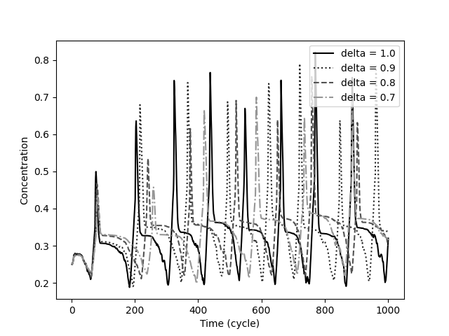
Arbitrary Constant $\beta$ : $\beta$ is an arbitrary constant that can be served to control the intensity of the inhibitory and enhancing signals. The value of $\beta$ is initially set to 1 for most experiments. Figure 9(a) shows a protein dynamic selected as a base dynamic to compare the impact of different initial states. Figure 9(b) illustrates how different $\beta$ values changes the dynamics for Protein 1. With an increase in the $\beta$ value, a shift in the generated patterns can be seen in time in a way that the same patterns happen later in the regulatory cycles but on a smaller scale. For $\beta=1.3$, the development is so slow that only one spike pattern can be observed during 1000 cycles compared to the eight spike patterns of $\beta=1$.

$\delta$ Arbitrary Constant : This constant value controls the intensity of protein production and is multiplied by the production signal at each development cycle. Same as $\beta$, the initial value of $\delta$ is set to 1. Figure 9(c) compares different $\delta$ values and their impact on the generated dynamics. A shift in time for the generated patterns can be seen for less $\delta$ values. In other words, lower $\delta$ values expand the produced dynamics while higher $\delta$ values shrink it. This impact is the opposite of the impact of $\beta$ on the dynamics. Also, unlike $\beta$, the concentration levels seem not to change as much, and the scale of the dynamics remains closer to the original one.

Initial Protein Concentration Levels: The initial concentration levels of the proteins were set to $\frac{1}{N}$ ($N$ is the number of genes) for most of our experiments. Here, an experiment was conducted to see the impact of these initial conditions by trying 0 and random initial levels. For the case that initial concentrations are set to 0 (Figure 9(d)), no change in the produced dynamics can be observed. Although not included in the graph, different constant values for initial concentrations were attempted. However, in all cases where the initial concentration levels were similar for all the proteins, no change in dynamics could be observed. Setting initial concentration levels to a random value resulted in a similar dynamic with the same patterns slightly shifted in different directions.

Starting TF Count: Another interesting factor to study is the impact of the initial number of TFs for each gene on the produced dynamics. It can be observed in Figure 9(e) that a change in the TF counts causes a shift in time and scale of the produced dynamics. It is worth noting that, unlike the case for $\beta$ and $\delta$ the time shift seems random and happens in both directions. An early appearance of the spike pattern happens in approximately cycle 60, where as the pattern occurs in a latter stage around approximately cycle 220.

Cell/Grid Size: The same as the case for different TF values, a shift in time and scale can be seen for different cell sizes (Figure 9(f)). The randomness in the scale and time shift is due to the random movements of the TFs. The larger the cell is, the longer it takes for the TFs to spread in the grid and to help the network to stabilize.

Changing Spatial Position of the Regulatory Sites: The proposed system is robust. Changing most initial states of the system, do not alter the shape of the generated patterns, but alters their scale or shifts them in time. However, a slight change in the position of the regulatory sites in the 2D grid, might significantly change the dynamics produced. In Figure 10 the enhancer position of gene 1 of the same network from Figure 9(a) is moved one unit away from its original position. A different protein concentration dynamic is generated in which the concentration level of proteins 1 and 3 stabilize to a value close to 0 in early cycles and concentration levels of proteins 2 and 4 produce an oscillatory pattern. Similar experiment was made on the other regulatory sites of different networks. In most cases, the dynamics drastically change; however, there are cases in which the dynamics slightly shift or do not change at all.

So far, the nature of the proposed system has been explained, and the different dynamics produced from random genomes generated from random seeds have been studied. However, to apply the proposed ARN in other applications, it is essential for this system to be evolvable to achieve desired dynamics. In this section, two experiments were conducted to evolve regulatory networks that meet a specific dynamic criterion. To evolve these networks, a simple GA was used that alters the initial DNA genotype of each individual. The utilized GA consists of a population of genome, one-point crossover, point mutation, and tournament as the selection mechanism. For both evolutionary experiments, a population size of 25, a mutation rate of 0.10, and a tournament size of 3 were configured. Each experiment was run for 50 generations.

In problem 1, the goal is for Protein 1 to reach a 0.085 concentration level at cycle 100. Figure 11(a) shows the evolutionary results for this problem. The X-axis is time, and the Y-axis is the deviation from the goal concentration in the form of absolute error. Therefore, lower values indicate a better individual. The depicted line represents the median fitness for the experiment’s 10 parallel runs, and the shaded areas represent the 75 and 25 quantiles. Figure 11(b) illustrates one of the evolved solutions for solving this problem. Several proteins share the same concentration levels.

In problem 2, the goal is for proteins 1 and 2 to alternate in concentration levels every 50 cycles so that in the starting period if protein 1 has more concentration than protein 2, the individual will be rewarded by 1 point. The individual receives another reward if, in the next period, protein 2 has more concentration than 1. The same level alteration process should continue for 10 cycle periods to achieve the maximum reward of 10. This is a more challenging task than problem 1, and the considered fitness function based on discrete rewards does not provide significant pressure towards solving the problem. Figure 11(c) shows the evolutionary results for solving problem 2. Although the median of individuals does not solve the problem, some cases fully solve it in 50 generations. Figure 11(d) shows a perfect solution to the problem achieved during evolution by one of the runs with fitness equal to 10.

Lastly, we conduct an experiment in which an attempt is made to depict the impact of point mutations on the outcome of the dynamics. Mutations occurring on different sites result in different behaviors, and their impact highly depends on the rest of the expressed genome. A single point-mutation on the protein-coding site can sometimes completely change the system’s dynamics, while sometimes it serves as a neutral mutation. In general, during the experiments, three significant outcomes from mutations could be observed in the system: 1- a neutral mutation, 2- a complete change in the dynamics, and 3- a shift in the scale and time of the dynamics. Figure 12 shows the concentration levels of only protein 1 from the entire dynamic of 9(a) undergoing 0 to 5 point mutations on the regulatory sites of the expressed genes. In the case of only one mutation, the concentration dynamics shrink, and more of the same spike patterns can be seen in the same number of cycles. In the case of two mutations, the dynamic expands, and only two of the spike patterns occur. The case of 3 mutations completely changes the dynamics, although the fourth mutation does not change the dynamics any further. It can be seen that more mutations have a higher probability of changing the dynamics entirely.

References

- [1] F. Muggianu, A. Benso, R. Bardini, E. Hu, G. Politano, and S. Di Carlo, “Modeling biological complexity using biology system description language (bisdl),” in 2018 IEEE International Conference on Bioinformatics and Biomedicine (BIBM), pp. 713–717, IEEE, 2018.
- [2] G. Theraulaz, E. Bonabeau, S. C. Nicolis, R. V. Solé, V. Fourcassié, S. Blanco, R. Fournier, J.-L. Joly, P. Fernández, A. Grimal, et al., “Spatial patterns in ant colonies,” Proceedings of the National Academy of Sciences, vol. 99, no. 15, pp. 9645–9649, 2002.
- [3] S. B. Carroll, “Endless forms most beautiful: The new science of evo devo and the making of the animal kingdom,” WW Norton & Company, vol. 54, 2005.
- [4] J. D. Watson and A. Berry, DNA: The Secret of Life. Knopf, 2009.
- [5] C. R. Calladine, H. Drew, B. Luisi, and A. Travers, Understanding DNA: The Molecule and How It Works. Academic Press, 3 ed., 2004.
- [6] L. A. Pennacchio, W. Bickmore, A. Dean, M. A. Nobrega, and G. Bejerano, “Enhancers: five essential questions,” Nature Reviews Genetics, vol. 14, no. 4, pp. 288–295, 2013.
- [7] M. Levine and E. H. Davidson, “Gene regulatory networks for development,” Proceedings of the National Academy of Sciences, vol. 102, pp. 4936–4942, mar 2005.
- [8] P. Gnanakkumaar, R. Murugesan, and S. S. S. J. Ahmed, “Gene regulatory networks in peripheral mononuclear cells reveals critical regulatory modules and regulators of multiple sclerosis,” Scientific Reports, vol. 9, sep 2019.
- [9] C. F. Arias, P. Catalán, S. Manrubia, and J. A. Cuesta, “toyLIFE: a computational framework to study the multi-level organisation of the genotype-phenotype map,” Scientific Reports, vol. 4, dec 2014.
- [10] M. Ruth and B. Hannon, “Modeling dynamic biological systems,” in Modeling Dynamic Biological Systems, pp. 3–27, Springer, 1997.
- [11] M. A. Deakin, “Modelling biological systems,” in Dynamics of Complex Interconnected Biological Systems, pp. 2–16, Springer, 1990.
- [12] D. J. Wilkinson, “Stochastic modelling for quantitative description of heterogeneous biological systems,” Nature Reviews Genetics, vol. 10, no. 2, pp. 122–133, 2009.
- [13] A. F. Villaverde, C. Cosentino, A. Gábor, and G. Szederkényi, “Computational methods for identification and modelling of complex biological systems,” Complexity, vol. 2019, 2019.
- [14] Y. Mohamadou, A. Halidou, and P. T. Kapen, “A review of mathematical modeling, artificial intelligence and datasets used in the study, prediction and management of covid-19,” Applied Intelligence, vol. 50, no. 11, pp. 3913–3925, 2020.
- [15] G. A. Wainer, Discrete-event modeling and simulation: a practitioner’s approach. CRC press, 2017.
- [16] M. Holcombe, S. Adra, M. Bicak, S. Chin, S. Coakley, A. I. Graham, J. Green, C. Greenough, D. Jackson, M. Kiran, et al., “Modelling complex biological systems using an agent-based approach,” Integrative Biology, vol. 4, no. 1, pp. 53–64, 2012.
- [17] W. Banzhaf, “On the dynamics of an artificial regulatory network,” in Advances in Artificial Life, pp. 217–227, Springer Berlin Heidelberg, 2003.
- [18] P. Dittrich, J. Ziegler, and W. Banzhaf, “Artificial chemistries—a review,” Artificial Life, vol. 7, pp. 225–275, jul 2001.
- [19] T. J. Hutton, “Evolvable self-replicating molecules in an artificial chemistry,” Artificial life, vol. 8, no. 4, pp. 341–356, 2002.
- [20] J. C. Astor and C. Adami, “A developmental model for the evolution of artificial neural networks,” Artificial life, vol. 6, no. 3, pp. 189–218, 2000.
- [21] P. Dittrich, J. Ziegler, and W. Banzhaf, “Mesoscopic analysis of an artificial chemistry with self-organizing topology,” 1998.
- [22] G. Kruszewski and T. Mikolov, “Emergence of self-reproducing metabolisms as recursive algorithms in an artificial chemistry,” Artificial Life, vol. 27, no. 3–4, pp. 277–299, 2022.
- [23] J. L. Schiff, Cellular automata: a discrete view of the world. John Wiley & Sons, 2011.
- [24] G. Karlebach and R. Shamir, “Modelling and analysis of gene regulatory networks,” Nature Reviews Molecular Cell Biology, vol. 9, pp. 770–780, sep 2008.
- [25] L. Glass and S. A. Kauffman, “The logical analysis of continuous, non-linear biochemical control networks,” Journal of Theoretical Biology, vol. 39, pp. 103–129, apr 1973.
- [26] I. Shmulevich, E. R. Dougherty, S. Kim, and W. Zhang, “Probabilistic boolean networks: a rule-based uncertainty model for gene regulatory networks,” Bioinformatics, vol. 18, pp. 261–274, feb 2002.
- [27] C. Chaouiya, A. Naldi, and D. Thieffry, “Logical modelling of gene regulatory networks with GINsim,” in Bacterial Molecular Networks, pp. 463–479, Springer New York, oct 2011.
- [28] S. Cussat-Blanc, K. Harrington, and W. Banzhaf, “Artificial gene regulatory networks—a review,” Artificial life, vol. 24, no. 4, pp. 296–328, 2019.
- [29] P. J. Bentley, “Evolving fractal proteins,” in International Conference on Evolvable Systems, pp. 81–92, Springer, 2003.
- [30] A. Chavoya and Y. Duthen, “A cell pattern generation model based on an extended artificial regulatory network,” Biosystems, vol. 94, no. 1-2, pp. 95–101, 2008.
- [31] S. Cussat-Blanc and J. Pollack, “Using pictures to visualize the complexity of gene regulatory networks,” in ALIFE 2012: The Thirteenth International Conference on the Synthesis and Simulation of Living Systems, pp. 491–498, MIT Press, 2012.
- [32] P. J. Bentley, “Evolving beyond perfection: An investigation of the effects of long-term evolution on fractal gene regulatory networks,” Biosystems, vol. 76, no. 1-3, pp. 291–301, 2004.
- [33] M. Joachimczak and B. Wróbel, “Evolution of the morphology and patterning of artificial embryos: scaling the tricolour problem to the third dimension,” in European Conference on Artificial Life, pp. 35–43, Springer, 2009.
- [34] J. C. Bongard and R. Pfeifer, “Evolving complete agents using artificial ontogeny,” in Morpho-functional Machines: The New Species, pp. 237–258, Springer, 2003.
- [35] N. R. Asr and V. J. Majd, “A new artificial genetic regulatory network model and its application in two dimensional robot control,” International Journal of Information and Electronics Engineering, vol. 3, no. 5, p. 461, 2013.
- [36] S. Sanchez and S. Cussat-Blanc, “Gene regulated car driving: using a gene regulatory network to drive a virtual car,” Genetic Programming and Evolvable Machines, vol. 15, no. 4, pp. 477–511, 2014.
- [37] B. Wróbel, A. Abdelmotaleb, M. Joachimczak, et al., “Evolving spiking neural networks in the greans (gene regulatory evolving artificial networks) platform,” in EvoNet2012: Evolving Networks, from Systems/Synthetic Biology to Computational Neuroscience Workshop at Artificial Life XIII, pp. 19–22, 2012.
- [38] B. Wróbel and M. Joachimczak, “Using the genetic regulatory evolving artificial networks (greans) platform for signal processing, animat control, and artificial multicellular development,” in Growing Adaptive Machines, pp. 187–200, Springer, 2014.
- [39] F. Jin, Y. Li, B. Ren, and R. Natarajan, “Enhancers: multi-dimensional signal integrators,” Transcription, vol. 2, no. 5, pp. 226–230, 2011.
- [40] W. Banzhaf and L. Yamamoto, “Basic concepts of artificial chemistries,” in Artificial Chemistries, pp. 11–44, The MIT Press, aug 2015.