An arbitrary order Reconstructed
Discontinuous Approximation to Fourth-order Curl Problem
Ruo Li
CAPT, LMAM and School of Mathematical
Sciences, Peking University, Beijing 100871, P.R. China
[email protected], Qicheng Liu
School of Mathematical
Sciences, Peking University, Beijing 100871, P.R. China
[email protected] and Shuhai Zhao
School of Mathematical
Sciences, Peking University, Beijing 100871, P.R. China
[email protected]
Abstract.
We present an arbitrary order discontinuous Galerkin finite element
method for solving the fourth-order curl problem using a reconstructed
discontinuous approximation method. It is based on an arbitrarily high-order
approximation space with one unknown
per element in each dimension. The discrete
problem is based on the symmetric IPDG method. We prove
a priori error estimates under the energy norm and the
norm and show numerical results to verify the theoretical analysis.
keywords: fourth-order curl problem,
patch reconstruction, discontinuous Galerkin method
1. Introduction
We are concerned in this paper with the fourth-order curl problem,
which has applications in inverse electromagnetic
scattering, and magnetohydrodynamics (MHD) when modeling magnetized
plasmas.
Discretizing the fourth-order curl operator is one of the keys to
simulate these models.
Additionally, the fourth-order curl operator plays an important role in
approximating the Maxwell transmission eigenvalue problem.
Therefore, it is important to design highly efficient and accurate
numerical methods for fourth-order curl problems
[2, 17].
Finite element methods (FEMs) are a widely used numerical scheme for
solving partial differential equations.
The design of FEMs for fourth-order curl problems is challenging. Nevertheless,
in recent years, researchers have proposed and analysed various
FEMs for these problems to address this difficulty. According to
whether the finite element space is contained within the space of the
exact solution, finite element methods can be classified into
conforming methods and nonconforming methods. For conforming methods,
one needs to construct -conforming finite elements, we
refer to [22, 6] for some recent works.
Due to the high order of the fourth-order curl operator, it is still a
difficult task to implement a high-order conforming space. Therefore,
many researches focus on nonconforming methods. The discontinuous
Galerkin (DG) methods use completely discontinuous piecewise
polynomial to approximate the solution of partial differential
equations. These methods enforce numerical solutions to be close to
the exact solution by adding penalties. DG methods are
commonly used in solving complex problems due to their simplicity and
flexibility in approximation space. For fourth-order curl
problems, we refer to [24, 5, 21, 20, 23] for some DG methods.
A significant drawback of DG methods is the large number of degrees of
freedom in DG space, which results in high computational costs. This
drawback is a matter of concern.
In this paper, we propose an arbitrary order discontinuous Galerkin
FEM for solving the fourth-order curl problem.
The method is based on a reconstructed approximation space
that has only one unknown per dimension in each element. The
construction of the approximation space includes
creating an element patch per element and solving a local least
squares fitting problem to obtain a local high-order polynomial.
Methods based on the reconstructed spaces are called reconstructed
discontinuous approximation (RDA) methods, which have been
successfully applied to a series of classical problems
[13, 10, 16, 15, 8, 14].
The reconstructed space is a subspace of the standard DG space,
which can approximate functions to high-order accuracy and
inherits the flexibility on the mesh partition in the meanwhile. One advantage of this
space is that it has very few degrees of freedom, which gives high
approximation efficiency of finite element.
Using this new space, we design the discrete scheme for the
fourth-order curl problem under the symmetric interior penalty
discontinuous Galerkin (IPDG) framework.
We prove the convergence rates under
the energy norm and the norm, and numerical experiments
are conducted to verify the theoretical analysis ,showing our
algorithm is simple to implement and can reach high-order accuracy.
The rest of this paper is organized as follows. In Section
2, we introduce the fourth-order curl problem without div-free condition
and give the basic notations about the Sobolev spaces and the
partition. We also recall two commonly used inequalities in this
section. In Section 3, we establish the reconstruction
operator and the corresponding approximation space. Some basic
properties of the reconstruction are also proven. In
Section 4, we define the discrete
variational form for the fourth-order curl problem and analyse the error
under the energy norm and the norm, and prove that the convergence
rate is optimal with respect to the energy norm. In Section
5, we carried out some numerical examples to
validate our theoretical results. Finally, a brief conclusion is given in Section
6.
2. Preliminaries
Let be a bounded polygonal
(polyhedral) domain with a Lipschitz boundary .
Given a bounded domain , we follow the standard
definitions to the space , the spaces with the regular exponent . The corresponding
norms and seminorms are defined as
respectively.
Throughout this paper, for two vectors , the cross product
is defined as
The cross product between a vector and a scalar will be
used in two dimensions, and in this case for a vector and a scalar , is
defined as .
Specifically, for a vector-valued function ,
the curl of reads
and for the scalar-valued function , we let
be the formal adjoint, which reads
For convenience, we mainly use the notations for the three-dimensional
case.
In this paper, we consider the following fourth-order curl problem
(1)
For the problem domain , we define the space
and
For the weak formulation we are going to find
such that
where
We refer to [18, 23] for some regularity results of this problem.
Next, we define some notations about the mesh. Let be a regular
and quasi-uniform partition into disjoint open triangles
(tetrahedra). Let denote the set of all
dimensional faces of , and we decompose into , where and are the
sets of interior faces and boundary faces, respectively. We let
and define .
The quasi-uniformity of the mesh is in the sense that there
exists a constant such that , where is the diameter of the
largest ball inscribed in . One can get the inverse inequality and
the trace inequality from the regularity of the mesh, which are
commonly used in the analysis.
Lemma 1.
There exists a constant independent of the mesh size , such that
(2)
Lemma 2.
There exists a constant independent of the mesh size , such that
(3)
where is the space of polynomial on with the
degree no more than .
We refer to [1] for more details of these
inequalities.
Finally, we introduce the trace operators that will be used in our
numerical schemes. For , we denote by and the
two neighbouring elements that share the boundary , and
the unit out normal vector on , respectively. We define the jump
operator and the average operator as
(4)
For , we let such that
and is the unit out normal vector. We define
(5)
Throughout this paper, and with subscripts denote the generic
constants that may differ between lines but are independent of the
mesh size.
3. Reconstructed Discontinuous Space
In this section, we will introduce a linear reconstruction operator to
obtain a discontinuous approximation space for the given mesh .
The reconstructed space can achieve a high-order accuracy while the
number of degrees of freedom in each dimension remain the same as the number of
elements in . The construction of the operator includes the
following steps.
Step 1. For each , we construct an element patch ,
which consists of itself and some surrounding elements.
The size of the patch is controlled with a given threshold .
The construction of the element patch is conducted by a
recursive algorithm. We begin by setting , and
define recursively:
(6)
where . The recursion stops once meets the condition
that the cardinality , and we let the patch
. We apply the recursive algorithm (6)
to all elements in .
Step 2. For each , we solve a local least squares fitting
problem on the patch . We let be the barycenter of
the element and mark barycenters of all elements as
collocation points.
Let be the set of collocation points located inside the domain
of ,
Let be the piecewise constant space with respect to ,
and we denote by the vector-valued
piecewise constant space. Given a function
and an integer , for the element ,
we consider the following local constrained least squares problem:
(7)
where denotes the set of collocation points located in ,
and denotes the discrete norm for vectors.
We make the following
geometrical assumption on the location of collocation points
[11, 10]:
Assumption 1.
For any element patch and any polynomial , implies .
The Assumption 1 excludes the case that the points in
are on an algebraic curve of degree and requires
cardinality . Under this
assumption, the fitting problem (7) admits a unique
solution.
By solving (7) and considering
the restriction , we actually gain a local
polynomial defined on . Since is sought in the
least squares sense, we note that depends linearly
on the given function . This property inspires us to define
a linear operator from the piecewise constant space to a
piecewise polynomial space with respect to .
We define a local reconstruction
operator for elements in ,
Further, the linear reconstruction operator for
is defined in a piecewise manner as
where is the image space of the operator
. Clearly, by the operator , any
piecewise constant function will be mapped into a piecewise
polynomial function . Then, we
present more details to the space , which are
piecewise polynomial spaces for the partition .
For any element , we pick up a function such that
where is the unit vector in whose -th entry
is . We let and we state that the space
is spanned by .
Lemma 3.
the functions are linearly independent
and the space .
Proof.
For any , assume there exists a group of coefficients
such that
(8)
From the constraint to the problem (7), we have
that
We choose for all in
(8), and it can be seen that . Thus,
the functions are linearly independent. Obviously, there holds
, and we note that the
dimension of is . By the
linear property of , we have that the space
is spanned by . This completes the
proof.
∎
Lemma 3 claims that the basis functions of
are indeed the group of functions , and for any function , one can explicitly write as
(9)
From the problem (7), the basis function
vanishes on the element that . This fact indicates has a finite
support set that , and is
different from the patch .
We extend the operator to act on smooth
functions. For any , we define a
piecewise constant function as
and we directly define . In this
way, any smooth function in is mapped into a
piecewise polynomial function with respect to by the operator
. For any ,
can also be written as (9).
Next, we will focus on the approximation property of the operator
. We first define a constant
for every element patch,
Assumption 1 as well as the norm equivalence in finite dimensional spaces
actually ensures .
Lemma 4.
For any element , there holds
(10)
Proof.
We define a polynomial space
Clearly, any polynomial in satisfies the
constraint to (7). Since is the solution to (7), for any
and
any , we
have that and
Because is arbitrary, the above inequality implies
for any . By letting and applying Cauchy-Schwarz inequality,
and we obtain
(11)
Combining the definition of the constant, we get
hence
and completes the proof.
∎
Assumption 2.
For every element patch ,
there exist constants and which are independent of such
that , and is star-shaped
with respect to , where is a disk with the radius
.
From the stability result (10), we can prove the
approximation results.
Lemma 5.
For any , there exists a constant such
that
(12)
for any , where we set
(13)
Proof.
According to Assumption2, there exists a polynomial , such that
Combining the stablility result of the reconstruction operator, we have
By the arbitraryness of ,
the case follows from the inverse inequality
∎
From (12), it can be seen that the operator
has an approximation error of degree under
the case that admits an upper bound
independent of the mesh size . However, it is not trivial to bound
the constant , see Remark 1. We can
prove that under some mild conditions on the element patch, the
constant admits a uniform upper bound.
It can be shown that . Hence when the constant
is uniformly bounded, so is .
For the patch , consider the special case that the
corresponding collocation points set has that , then the constant is
equal to the Lebesgue constant [19] and
the solution to the least squares problem (7) is
just the Lagrange interpolation polynomial, however, in this case the constant
may depend on and grow very fast, which will
further damage the convergence. To ensure the stability of the reconstruction
operator, we are acquired to
choose a sufficiently large so that the constant
admits a uniform upper bound, thus. We refer to
[10, Lemma 6] and
[11, Lemma 3.4] for the details of this statement.
The wide element patch will bring more computational cost
for filling the stiffness matrix and increase the width of the
banded structure. This is just the price we have to pay for the
uniform bound of .
4. Approximation to Fourth-order Curl Problem
We define the approximation problem to solve the
problem (1) based on the space constructed in
the previous section: Seek () such that
The parameter and are positive penalties which are set
by
The linear form is defined for ,
We introduce two energy norms for the space ,
and
We claim that the two energy norms are equivalent over the space
.
Lemma 6.
For any , there exists a constant , such that
(15)
Proof.
We only need to prove . For , we denote the two neighbor elements of by and
. We have
By the trace inequalities (2),
and the inverse inequality (3), we obtain that
For , let . Similarly, we have
The term can bounded by the
same way. Thus, by summing over all ,
we conclude that
which can immediately leads us to (15) and completes
the proof.
∎
Now we are ready to prove the coercivity and the continuity of the
bilinear form .
Theorem 1.
Let be the bilinear form with sufficiently large
penalty . Then there exists a positive constant such that
(16)
Proof.
From Lemma 15, we only need to establish the coercivity
over the norm . For the face , let
be shared by the neighbor elements and . We apply the
Cauchy-Schwarz inequality,
for any . From the trace inequalities
(2), and the inverse inequality
(3), we deduce that
Thus, we have
(17)
For the face , we can similarly derive that
(18)
By employing the same method to the term , we can obtain that
(19)
Combining the inequalities (17), (18),
(19), we conclude that
there exists a constant such that
for any . We can let and
select a sufficiently large to ensure , which completes the proof.
∎
Theorem 2.
There exists a positive constant such that
(20)
Proof.
By directly using the Cauchy-Schwarz
inequality,
which completes the proof.
∎
Now we verify the Galerkin orthogonality.
Lemma 7.
Suppose is the exact solution to
the problem (1), and is the
numerical solution to the discrete problem (14),
then
(21)
Proof.
We first have for the two jump terms
Taking the exact solution into , we have that
We multiply the test function at both side of equation
(1), and apply the integration by parts to get
Thus, by simply calculating, we obtain that
which completes the proof.
∎
Then we establish the interpolation error estimate of the reconstruction
operator.
Lemma 8.
For and , there exists a constant
such that
(22)
Proof.
From Lemma
LABEL:le_localapproximation, we can show that
,also
By the trace estimate (2) and the mesh regularity,
and
which completes the proof.
∎
Now we are ready to present the a priori error estimate under
within the standard Lax-Milgram framework.
Theorem 3.
Suppose the problem (1) has a
solution , where , and has a uniform upper bound
independent of .
Let the bilinear form be defined with a
sufficiently large and be the numerical
solution to the problem (14). Then for there exists a constant such that
Under the same assumptions, there exists a constant such that
(24)
Remark 2.
We have proved that under the energy norm the
numerical solution
has the optimal convergence rate. It can be seen that
is stronger than
from the definition of . Hence, from
(24) we can conclude that the numerical
solution at least have the
convergence rate in norm, which is exactly the convergence rate indicated
by our numerical tests.
5. Numerical Results
In this section, we conduct a series numerical experiments to test the
performance of our method. For the accuracy , the
threshold we used in the examples
are listed in Tab. 1. For all examples,
the boundary and the right hand side
in the equation (1) are chosen according to the
exact solution.
Example 1.
We first consider a fourth-order curl problem defined on the squared domain
. The exact solution is chosen by
We solve the problem on a sequence of meshes with the size
. The convergence histories under
the (which is equivalent to )and
are shown in
Fig. 1. The error under the energy norm is decreasing
at the speed for fixed . For error, the speed is
the same as the energy norm. These results
coincide with the theoretical analysis in Theorem
24 .
2
3
4
12
20
27
2
3
25
47
Table 1. The used in 2D and 3D examples.
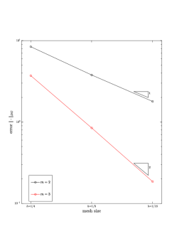
Figure 1. The convergence histories under the
(left) and the (right) in Example 1.
Example 2.
We solve a three-dimensional problem in this
case. The computation domain is an unit cube
.
We select the exact solution as
We use the tetrahedra meshes generated by the Gmsh software
[3]. We solve the problem on three different meshes
with the reconstruction order . The convergence order
in both norms is shown in
Fig. 2, also consistent with our
theoretical predictions.
Figure 2. The convergence histories under the
(left) and the (right) in Example 2.
6. Conclusion
In this paper, we proposed an IPDG method
for the fourth-order curl problem with the reconstructed discontinuous
approximation. The approximation space is based on
patch reconstruction from piecewise constant sapce and can approximate
functions up to high order accuracy. We show numercial experiments
in two and three dimensions to examine the order of convergence under the energy
norm and the norm.
Appendix A Calculating the Reconstruction Constant
This appendix gives the method to compute the constant
for a given mesh . For any element , let be a group of standard orthogonal basis functions
in under the inner product . Then, any polynomial can be
expanded by a group coefficients such that . We can naturally extend and all
to the domain by the polynomial extension. The main step to
get is to compute for all elements, and
can be represented as
From the matrix representation, , where is the
smallest singular value to .
Hence, it is enough to observe the
minimum value of for all elements, and
can be computed by (13).
As we remarked in Section 3, when the patch is wide
enough, will admit a uniform upper bound independent of
the mesh size. Here, we will show for different size of
the patch. We consider the triangular mesh with
and the tetrahedral mesh with in two and three
dimensions, which are used in Example 1 and Example 2.
The values of are collected in Fig. 3.
Figure 3. in 2d with (row 1) /
in 3d with (row 2).
References
[1]
S. C. Brenner and L. R. Scott, The Mathematical Theory of Finite Element
Methods, third ed., Texts in Applied Mathematics, vol. 15, Springer, New
York, 2008.
[2]
Fioralba Cakoni and Houssem Haddar, A variational approach for the
solution of the electromagnetic interior transmission problem for anisotropic
media, Inverse Problems and Imaging 1 (2007), 443–456.
[3]
C. Geuzaine and J. F. Remacle, Gmsh: A 3-D finite element mesh
generator with built-in pre- and post-processing facilities, Internat. J.
Numer. Methods Engrg. 79 (2009), no. 11, 1309–1331.
[4]
Jiayu Han and Zhimin Zhang, An hp-version interior penalty discontinuous
galerkin method for the quad-curl eigenvalue problem, BIT Numerical
Mathematics 63 (2023), article number 56.
[5]
Qingguo Hong, Jun Hu, Shi Shu, and Jinchao Xu, A discontinuous galerkin
method for the fourth-order curl problem, Journal of Computational
Mathematics 30 (2012), 565–578.
[6]
Kaibo Hu, Qian Zhang, and Zhimin Zhang, Simple curl-curl-conforming
finite elements in two dimensions, SIAM Journal on Scientific Computing
42 (2020), no. 6, A3859–A3877.
[7]
T. J. R. Hughes, G. Engel, L. Mazzei, and M. G. Larson, A comparison of
discontinuous and continuous Galerkin methods based on error estimates,
conservation, robustness and efficiency, Discontinuous Galerkin methods
(Newport, RI, 1999), Lect. Notes Comput. Sci. Eng., vol. 11, Springer,
Berlin, 2000, pp. 135–146.
[8]
R. Li, Q. Liu, and F. Yang, A reconstructed discontinuous approximation
on unfitted meshes to and interface
problems, Comput. Methods Appl. Mech. Engrg. 403 (2023), no. part
A, Paper No. 115723, 27.
[9]
R. Li, P. Ming, Z. Sun, F. Yang, and Z. Yang, A discontinuous Galerkin
method by patch reconstruction for biharmonic problem, J. Comput. Math.
37 (2019), no. 4, 563–580.
[10]
R. Li, P. Ming, Z. Sun, and Z. Yang, An arbitrary-order discontinuous
Galerkin method with one unknown per element, J. Sci. Comput. 80
(2019), no. 1, 268–288.
[11]
R. Li, P. Ming, and F. Tang, An efficient high order heterogeneous
multiscale method for elliptic problems, Multiscale Model. Simul.
10 (2012), no. 1, 259–283.
[12]
R. Li, Z. Sun, and F. Yang, Solving eigenvalue problems in a
discontinuous approximate space by patch reconstruction, SIAM J. Sci.
Comput. 41 (2019), no. 5, A3381–A3400.
[13]
R. Li and F. Yang, A discontinuous Galerkin method by patch
reconstruction for elliptic interface problem on unfitted mesh, SIAM J. Sci.
Comput. 42 (2020), no. 2, A1428–A1457.
[14]
by same author, A least squares method for linear elasticity using a patch
reconstructed space, Comput. Methods Appl. Mech. Engrg. 363 (2020),
no. 1, 112902.
[15]
by same author, A sequential least squares method for Poisson equation using a
patch reconstructed space, SIAM J. Numer. Anal. 58 (2020), no. 1,
353–374.
[16]
by same author, A reconstructed discontinuous approximation to
Monge-Ampère equation in least square formulation, Adv. Appl. Math.
Mech. 15 (2023), no. 5, 1109–1141. MR 4613677
[17]
Peter Monk and Jiguang Sun, Finite element methods for maxwell’s
transmission eigenvalues, SIAM Journal on Scientific Computing 34
(2012), B247–B264.
[18]
Serge Nicaise, Singularities of the quad curl problem, Journal of
Differential Equations 264 (2018), 5025–5069.
[19]
M. J. D. Powell, Approximation theory and methods, Cambridge University
Press, Cambridge-New York, 1981.
[20]
Jiguang Sun, A mixed fem for the quad-curl eigenvalue problem,
Numerische Mathematik 132 (2013), 185–200.
[21]
Jiguang Sun, Qian Zhang, and Zhimin Zhang, A curl-conforming weak
galerkin method for the quad-curl problem, BIT Numerical Mathematics
59 (2019), 1093–1114.
[22]
Qian Zhang, Lixiu Wang, and Zhimin Zhang, H()-conforming finite
elements in 2 dimensions and applications to the quad-curl problem, SIAM
Journal on Scientific Computing 41 (2019), A1527–A1547.
[23]
Shuo Zhang, Mixed schemes for quad-curl equations, ESAIM: Mathematical
Modelling and Numerical Analysis 52 (2018), 147–161.
[24]
Bin Zheng, Qiya Hu, and Jinchao Xu, A nonconforming finite element method
for fourth order curl equations in , Math. Comput. 80 (2010),
1871–1886.