This paper was converted on www.awesomepapers.org from LaTeX by an anonymous user.
Want to know more? Visit the Converter page.

\newdate

date912017

An approximate randomization test for high-dimensional two-sample Behrens-Fisher problem under arbitrary covariances

Rui Wang Center for Applied Statistics and School of Statistics, Renmin University of China, Beijing 100872, China Wangli Xu Corresponding author
Email address: [email protected] Center for Applied Statistics and School of Statistics, Renmin University of China, Beijing 100872, China
Abstract

This paper is concerned with the problem of comparing the population means of two groups of independent observations. An approximate randomization test procedure based on the test statistic of Chen and Qin, (2010) is proposed. The asymptotic behavior of the test statistic as well as the randomized statistic is studied under weak conditions. In our theoretical framework, observations are not assumed to be identically distributed even within groups. No condition on the eigenstructure of the covariance matrices is imposed. And the sample sizes of the two groups are allowed to be unbalanced. Under general conditions, all possible asymptotic distributions of the test statistic are obtained. We derive the asymptotic level and local power of the approximate randomization test procedure. Our theoretical results show that the proposed test procedure can adapt to all possible asymptotic distributions of the test statistic and always has correct test level asymptotically. Also, the proposed test procedure has good power behavior. Our numerical experiments show that the proposed test procedure has favorable performance compared with several alternative test procedures.

Key words: Behrens-Fisher problem; High-dimensional data; Randomization test; Lindeberg principle.

1 Introduction

Two-sample mean testing is a fundamental problem in statistics with an enormous range of applications. In modern statistical applications, high-dimensional data, where the data dimension may be much larger than the sample size, is ubiquitous. However, most classical two-sample mean tests are designed for low-dimensional data, and may not be feasible, or may have suboptimal power, for high-dimensional data; see, e.g., Bai and Saranadasa, (1996). In recent years, the study of high-dimensional two-sample mean tests has attracted increasing attention.

Suppose that Xk,iX_{k,i}, i=1,,nki=1,\ldots,n_{k}, k=1,2k=1,2, are independent pp-dimensional random vectors with E(Xk,i)=μk\operatorname{E}(X_{k,i})=\mu_{k}, var(Xk,i)=𝚺k,i\operatorname{var}(X_{k,i})=\bm{\Sigma}_{k,i}. The hypothesis of interest is

0:μ1=μ2v.s.1:μ1μ2.\displaystyle\mathcal{H}_{0}:\mu_{1}=\mu_{2}\quad\text{v.s.}\quad\mathcal{H}_{1}:\mu_{1}\neq\mu_{2}. (1)

Denote by ¯𝚺k=nk1i=1nk𝚺k,i\bar{}\bm{\Sigma}_{k}=n_{k}^{-1}\sum_{i=1}^{n_{k}}\bm{\Sigma}_{k,i} the average covariance matrix within group kk, k=1,2k=1,2. Most existing methods on two-sample mean tests assumed that the observations within groups are identically distributed. In this case, 𝚺k,i=¯𝚺k\bm{\Sigma}_{k,i}=\bar{}\bm{\Sigma}_{k}, i=1,,nki=1,\ldots,n_{k}, k=1,2k=1,2, and the considered testing problem reduces to the well-known Behrens-Fisher problem. In this paper, we consider the more general setting where the observations are allowed to have different distributions even within groups. Also, we consider the case where the data is possibly high-dimensional, that is, the data dimension pp may be much larger than the sample size nkn_{k}, k=1,2k=1,2.

Let X¯k=nk1i=1nkXk,i\bar{X}_{k}=n_{k}^{-1}\sum_{i=1}^{n_{k}}X_{k,i} and 𝐒k=(nk1)1i=1nk(Xk,iX¯k)(Xk,iX¯k)\mathbf{S}_{k}=(n_{k}-1)^{-1}\sum_{i=1}^{n_{k}}(X_{k,i}-\bar{X}_{k})(X_{k,i}-\bar{X}_{k})^{\intercal} denote the sample mean vector and the sample covariance matrix of group kk, respectively, k=1,2k=1,2. Denote n=n1+n2n=n_{1}+n_{2}. A classical test statistic for hypothesis (1) is Hotelling’s T2T^{2} statistic, defined as

n1n2n(X¯1X¯2)𝐒1(X¯1X¯2),\displaystyle\frac{n_{1}n_{2}}{n}(\bar{X}_{1}-\bar{X}_{2})^{\intercal}\mathbf{S}^{-1}(\bar{X}_{1}-\bar{X}_{2}),

where 𝐒=(n2)1{(n11)𝐒1+(n21)𝐒2}\mathbf{S}=(n-2)^{-1}\{(n_{1}-1)\mathbf{S}_{1}+(n_{2}-1)\mathbf{S}_{2}\} is the pooled sample covariance matrix. When p>n2p>n-2, the matrix 𝐒\mathbf{S} is not invertible, and consequently Hotelling’s T2T^{2} statistic is not well-defined. In a seminal work, Bai and Saranadasa, (1996) proposed the test statistic

TBS(𝐗1,𝐗2)=X¯1X¯22nn1n2tr(𝐒),\displaystyle T_{\mathrm{BS}}(\mathbf{X}_{1},\mathbf{X}_{2})=\|\bar{X}_{1}-\bar{X}_{2}\|^{2}{-\frac{n}{n_{1}n_{2}}\operatorname{tr}(\mathbf{S})},

where 𝐗k=(Xk,1,,Xk,nk)\mathbf{X}_{k}=(X_{k,1},\ldots,X_{k,n_{k}})^{\intercal} is the data matrix of group kk, k=1,2k=1,2. The test statistic TBS(𝐗1,𝐗2)T_{\mathrm{BS}}(\mathbf{X}_{1},\mathbf{X}_{2}) is well-defined for arbitrary pp. Bai and Saranadasa, (1996) assumed that the observations within groups are identically distributed and ¯𝚺1=¯𝚺2\bar{}\bm{\Sigma}_{1}=\bar{}\bm{\Sigma}_{2}. The main term of TBS(𝐗1,𝐗2)T_{\mathrm{BS}}(\mathbf{X}_{1},\mathbf{X}_{2}) is X¯1X¯22\|\bar{X}_{1}-\bar{X}_{2}\|^{2}. Chen and Qin, (2010) removed terms Xk,iXk,iX_{k,i}^{\intercal}X_{k,i} from X¯1X¯22\|\bar{X}_{1}-\bar{X}_{2}\|^{2} and proposed the test statistic

TCQ(𝐗1,𝐗2)=k=122i=1nkj=i+1nkXk,iXk,jnk(nk1)2i=1n1j=1n2X1,iX2,jn1n2.\displaystyle T_{\text{CQ}}(\mathbf{X}_{1},\mathbf{X}_{2})=\sum_{k=1}^{2}\frac{2\sum_{i=1}^{n_{k}}\sum_{j=i+1}^{n_{k}}X_{k,i}^{\intercal}X_{k,j}}{n_{k}(n_{k}-1)}-\frac{2\sum_{i=1}^{n_{1}}\sum_{j=1}^{n_{2}}X_{1,i}^{\intercal}X_{2,j}}{n_{1}n_{2}}.

The test method of Chen and Qin, (2010) can be applied when ¯𝚺1¯𝚺2\bar{}\bm{\Sigma}_{1}\neq\bar{}\bm{\Sigma}_{2}. Both Bai and Saranadasa, (1996) and Chen and Qin, (2010) used the asymptotical normality of the statistics to determine the critical value of the test. However, the asymptotical normality only holds for a restricted class of covariance structures. For example, Chen and Qin, (2010) assumed that

tr(¯𝚺k4)=o[[tr{(¯𝚺1+¯𝚺2)2}]2],k=1,2.\displaystyle\operatorname{tr}(\bar{}\bm{\Sigma}_{k}^{4})=o\left[[\operatorname{tr}\{(\bar{}\bm{\Sigma}_{1}+\bar{}\bm{\Sigma}_{2})^{2}\}]^{2}\right],\quad k=1,2. (2)

However, (2) may not hold when ¯𝚺k\bar{}\bm{\Sigma}_{k} has a few eigenvalues significantly larger than the others, excluding some important senarios in practice. For example, (2) is often violated when the variables are affected by some common factors; see, e.g., Fan et al., (2021) and the references therein. If the condition (2) is violated, the test procedures of Bai and Saranadasa, (1996) and Chen and Qin, (2010) may have incorrect test level; see, e.g., Wang and Xu, (2019). For years, how to construct test procedures that are valid under general covariances has been an important open problem in the field of high-dimensional hypothesis testing; see the review paper of Hu and Bai, (2016).

Intuitively, one may resort to the bootstrap method to control the test level under general covariances. Surprisingly, as shown by our numerical experiments, the empirical bootstrap method does not work well for TCQ(𝐗1,𝐗2)T_{\mathrm{CQ}}(\mathbf{X}_{1},\mathbf{X}_{2}). Also, the wild bootstrap method, which is popular in high-dimensional statistics, does not work well either. We will give heuristic arguments to understand this phenomenon in Section 3. Recently, several methods were proposed to give a better control of the test level of TCQ(𝐗1,𝐗2)T_{\mathrm{CQ}}(\mathbf{X}_{1},\mathbf{X}_{2}) and related test statistics. In the setting of ¯𝚺1=¯𝚺2\bar{}\bm{\Sigma}_{1}=\bar{}\bm{\Sigma}_{2}, Zhang et al., (2020) considered the statistic X¯1X¯22\|\bar{X}_{1}-\bar{X}_{2}\|^{2} and proposed to use the Welch-Satterthwaite χ2\chi^{2}-approximation to determine the critical value. Subsequently, Zhang et al., (2021) extended the test procedure of Zhang et al., (2020) to the two-sample Behrens-Fisher problem, and Zhang and Zhu, (2021) considered a χ2\chi^{2}-approximation of TCQ(𝐗1,𝐗2)T_{\mathrm{CQ}}(\mathbf{X}_{1},\mathbf{X}_{2}). However, the test methods of Zhang et al., (2020), Zhang et al., (2021) and Zhang and Zhu, (2021) still require certain conditions on the eigenstructure of ¯𝚺k\bar{}\bm{\Sigma}_{k}, k=1,2k=1,2. In another work, Wu et al., (2018) investigated the general distributional behavior of X¯12\|\bar{X}_{1}\|^{2} for one-sample mean testing problem. They proposed a half-sampling procedure to determine the critical value of the test statistic. A generalization of the method of Wu et al., (2018) to the statistc X¯1X¯22\|\bar{X}_{1}-\bar{X}_{2}\|^{2} for the two-sample Behrens-Fisher problem when both n1n_{1} and n2n_{2} are even numbers was presented in Chapter 2 of Lou, (2020). Unfortunately, Wu et al., (2018) and Lou, (2020) did not include detailed proofs of their theoretical results. Recently, Wang and Xu, (2019) considered a randomization test based on the test statistic of Chen and Qin, (2010) for the one-sample mean testing problem. Their randomization test has exact test level if the distributions of the observations are symmetric and has asymptotically correct level in the general setting. Although many efforts have been made, no existing test procedure based on TCQ(𝐗1,𝐗2)T_{\mathrm{CQ}}(\mathbf{X}_{1},\mathbf{X}_{2}) is valid for arbitrary ¯𝚺k\bar{}\bm{\Sigma}_{k} with rigorous theoretical guarantees.

The statistics TBS(𝐗1,𝐗2)T_{\mathrm{BS}}(\mathbf{X}_{1},\mathbf{X}_{2}) and TCQ(𝐗1,𝐗2)T_{\mathrm{CQ}}(\mathbf{X}_{1},\mathbf{X}_{2}) are based on sum-of-squares. Some researchers investigated variants of sum-of-squares statistics that are scalar-invariant; see, e.g., Srivastava and Du, (2008), Srivastava et al., (2013) and Feng et al., (2015). These test methods also impose some nontrivial assumptions on the eigenstructure of the covariance matrices. There is another line of research initiated by Cai et al., (2013) which utilizes extreme value type statistics to test hypothesis (1). Chang et al., (2017) considered a parametric bootstrap method to determine the critical value of the extreme value type statistics. The method of Chang et al., (2017) allows for general covariance structures. Recently, Xue and Yao, (2020) investigated a wild bootstrap method. The test procedure in Xue and Yao, (2020) does not require that the observations within groups are identically distributed. The theoretical analyses in Chang et al., (2017) and Xue and Yao, (2020) are based on recent results about high-dimensional bootstrap methods developed by Chernozhukov et al., (2013) and Chernozhukov et al., (2017). While their theoretical framework can be applied to extreme value type statistics, it can not be applied to sum-of-squares type statistics like TCQ(𝐗1,𝐗2)T_{\mathrm{CQ}}(\mathbf{X}_{1},\mathbf{X}_{2}). Indeed, we shall see that the wild bootstrap method does not work well for TCQ(𝐗1,𝐗2)T_{\mathrm{CQ}}(\mathbf{X}_{1},\mathbf{X}_{2}).

In the present paper, we propose a new test procedure based on TCQ(𝐗1,𝐗2)T_{\mathrm{CQ}}(\mathbf{X}_{1},\mathbf{X}_{2}). In the proposed test procedure, we use a new randomization method to determine the critical value of the test statistic. The proposed randomization method is motivated by the randomization method proposed in Fisher, (1935), Section 21. While this randomization method is widely used in one-sample mean testing problem, it can not be directly applied to two-sample Behrens-Fisher problem. In comparison, the proposed randomization method has satisfactory performance for two-sample Behrens-Fisher problem. We investigate the asymptotic properties of the proposed test procedure and rigorously prove that it has correct test level asymptotically under fairly weak conditions. Compared with existing test procedures based on sum-of-squares, the present work has the following favorable features. First, the proposed test procedure has correct test level asymptotically without any restriction on ¯𝚺k\bar{}\bm{\Sigma}_{k}, k=1,2k=1,2. As a consequence, the proposed test procedure serves as a rigorous solution to the open problem that how to construct a valid test based on TCQ(𝐗1,𝐗2)T_{\mathrm{CQ}}(\mathbf{X}_{1},\mathbf{X}_{2}) under general covariances. Second, the proposed test procedure is valid even if the observations within groups are not identically distributed. To the best of our knowledge, the only existing method that can work in such a general setting is the test procedure in Xue and Yao, (2020). However, the test procedure in Xue and Yao, (2020) is based on extreme value statistic, which is different from the present work. Third, our theoretical results are valid for arbitrary n1n_{1} and n2n_{2} as long as min(n1,n2)\min(n_{1},n_{2})\to\infty. In comparison, all the above mentioned methods only considered the balanced data, that is, the sample sizes n1n_{1} and n2n_{2} are of the same order. We also derive the asymptotic local power of the proposed method. It shows that the asymptotic local power of the proposed test procedure is the same as that of the oracle test procedure where the distribution of the test statistic is known. A key tool for the proofs of our theoretical results is a universality property of the generalized quadratic forms. This result may be of independent interest. We also conduct numerical experiments to compare the proposed test procedure with some existing methods. Our theoretical and numerical results show that the proposed test procedure has good performance in both level and power.

2 Asymptotics of TCQ(𝐗1,𝐗2)T_{\mathrm{CQ}}(\mathbf{X}_{1},\mathbf{X}_{2})

In this section, we investigate the asymptotic behavior of TCQ(𝐗1,𝐗2)T_{\mathrm{CQ}}(\mathbf{X}_{1},\mathbf{X}_{2}) under general conditions. We begin with some notations. For two random variables ξ\xi and ζ\zeta, let (ξ)\mathcal{L}(\xi) denote the distribution of ξ\xi, and (ξζ)\mathcal{L}(\xi\mid\zeta) denote the conditional distribution of ξ\xi given ζ\zeta. For two probability measures ν1\nu_{1} and ν2\nu_{2} on \mathbb{R}, let ν1ν2\nu_{1}-\nu_{2} be the signed measure such that for any Borel set 𝒜\mathcal{A}, (ν1ν2)(𝒜)=ν1(𝒜)ν2(𝒜)(\nu_{1}-\nu_{2})(\mathcal{A})=\nu_{1}(\mathcal{A})-\nu_{2}(\mathcal{A}). Let 𝒞b3()\mathscr{C}_{b}^{3}(\mathbb{R}) denote the class of bounded functions with bounded and continuous derivatives up to order 33. It is known that a sequence of random variables {ξn}n=1\{\xi_{n}\}_{n=1}^{\infty} converges weakly to a random variable ξ\xi if and only if for every f𝒞b3()f\in\mathscr{C}_{b}^{3}(\mathbb{R}), Ef(ξn)Ef(ξ)\operatorname{E}f(\xi_{n})\to\operatorname{E}f(\xi); see, e.g., Pollard, (1984), Chapter III, Theorem 12. We use this property to give a metrization of the weak convergence in \mathbb{R}. For a function f𝒞b3()f\in\mathscr{C}_{b}^{3}(\mathbb{R}), let f(i)f^{(i)} denote the iith derivative of ff, i=1,2,3i=1,2,3. For a finite signed measure ν\nu on \mathbb{R}, we define the norm ν3\|\nu\|_{3} as supf|df(𝐱)ν(d𝐱)|\sup_{f}\left|\int_{\mathbb{R}^{d}}f(\mathbf{x})\,\nu(\mathrm{d}\mathbf{x})\right|, where the supremum is taken over all f𝒞b3()f\in\mathscr{C}_{b}^{3}(\mathbb{R}) such that sup𝐱|f(x)|1\sup_{\mathbf{x}\in\mathbb{R}}|f(x)|\leq 1 and sup𝐱|f()(x)|1\sup_{\mathbf{x}\in\mathbb{R}}|f^{(\ell)}(x)|\leq 1, =1,2,3\ell=1,2,3. It is straightforward to verify that 3\|\cdot\|_{3} is indeed a norm for finite signed measures. Also, a sequence of probability measures {νn}n=1\{\nu_{n}\}_{n=1}^{\infty} converges weakly to a probability measure ν\nu if and only if νnν30\|\nu_{n}-\nu\|_{3}\to 0; see, e.g., Dudley, (2002), Corollary 11.3.4.

The test procedure of Chen and Qin, (2010) determines the critical value based on the asymptotic normality of TCQ(𝐗1,𝐗2)T_{\mathrm{CQ}}(\mathbf{X}_{1},\mathbf{X}_{2}) under the null hypothesis. Define Yk,i=Xk,iμkY_{k,i}=X_{k,i}-\mu_{k}, i=1,,nki=1,\ldots,n_{k}, k=1,2k=1,2. Then E(Yk,i)=𝟎p\operatorname{E}(Y_{k,i})=\mathbf{0}_{p}. Under the null hypothesis, we have TCQ(𝐗1,𝐗2)=TCQ(𝐘1,𝐘2)T_{\text{CQ}}(\mathbf{X}_{1},\mathbf{X}_{2})=T_{\text{CQ}}(\mathbf{Y}_{1},\mathbf{Y}_{2}) where 𝐘k=(Yk,1,,Yk,nk)\mathbf{Y}_{k}=(Y_{k,1},\ldots,Y_{k,n_{k}})^{\intercal}, k=1,2k=1,2. Denote by σT,n2\sigma_{T,n}^{2} the variance of TCQ(𝐘1,𝐘2)T_{\text{CQ}}(\mathbf{Y}_{1},\mathbf{Y}_{2}). Under certain conditions, Chen and Qin, (2010) proved that TCQ(𝐘1,𝐘2)/σT,nT_{\mathrm{CQ}}(\mathbf{Y}_{1},\mathbf{Y}_{2})/\sigma_{T,n} converges weakly to 𝒩(0,1)\mathcal{N}(0,1). They reject the null hypothesis if TCQ(𝐗1,𝐗2)/σ^T,nT_{\mathrm{CQ}}(\mathbf{X}_{1},\mathbf{X}_{2})/\hat{\sigma}_{T,n} is greater than the 1α1-\alpha quantile of 𝒩(0,1)\mathcal{N}(0,1) where σ^T,n\hat{\sigma}_{T,n} is an estimate of σT,n\sigma_{T,n} and α(0,1)\alpha\in(0,1) is the test level. However, we shall see that normal distribution is just one of the possible asymptotic distributions of TCQ(𝐘1,𝐘2)T_{\mathrm{CQ}}(\mathbf{Y}_{1},\mathbf{Y}_{2}) in the general setting.

Now we list the main conditions imposed by Chen and Qin, (2010) to prove the asymptotic normality of TCQ(𝐘1,𝐘2)T_{\mathrm{CQ}}(\mathbf{Y}_{1},\mathbf{Y}_{2}). First, Chen and Qin, (2010) imposed the condition (2) on the eigenstructure of ¯𝚺k\bar{}\bm{\Sigma}_{k}, k=1,2k=1,2. Second, Chen and Qin, (2010) assumed that as nn\to\infty,

n1/nb(0,1).\displaystyle{n_{1}}/{n}\to b\in(0,1). (3)

That is, Chen and Qin, (2010) assumed the sample sizes in two groups are balanced. This condition is commonly adopted by existing test procedures for hypothesis (1). Third, Chen and Qin, (2010) assumed the general multivariate model

Yk,i=𝚪kZk,i,i=1,,nk,k=1,2,\displaystyle Y_{k,i}=\bm{\Gamma}_{k}Z_{k,i},\quad i=1,\ldots,n_{k},\quad k=1,2, (4)

where 𝚪k\bm{\Gamma}_{k} is a p×mp\times m matrix for some mpm\geq p, k=1,2k=1,2, and {Zk,i}i=1nk\{Z_{k,i}\}_{i=1}^{n_{k}} are mm-dimensional independent and identically distributed random vectors such that E(Zk,i)=𝟎m\operatorname{E}(Z_{k,i})=\mathbf{0}_{m}, var(Zk,i)=𝐈m\operatorname{var}(Z_{k,i})=\mathbf{I}_{m}, and the elements of Zk,i=(zk,i,1,,zk,i,m)Z_{k,i}=(z_{k,i,1},\ldots,z_{k,i,m})^{\intercal} satisfy E(zk,i,j4)=3+Δ<\operatorname{E}(z_{k,i,j}^{4})=3+\Delta<\infty, and E(zk,i,1α1zk,i,2α2zk,i,qαq)=E(zk,i,1α1)E(zk,i,2α2)E(zk,i,qαq)\operatorname{E}(z_{k,i,\ell_{1}}^{\alpha_{1}}z_{k,i,\ell_{2}}^{\alpha_{2}}\cdots z_{k,i,\ell_{q}}^{\alpha_{q}})=\operatorname{E}(z_{k,i,\ell_{1}}^{\alpha_{1}})\operatorname{E}(z_{k,i,\ell_{2}}^{\alpha_{2}})\cdots\operatorname{E}(z_{k,i,\ell_{q}}^{\alpha_{q}}) for a positive integer qq such that =1qα8\sum_{\ell=1}^{q}\alpha_{\ell}\leq 8 and distinct 1,,q{1,,m}\ell_{1},\ldots,\ell_{q}\in\{1,\ldots,m\}. We note that the general multivariate model (4) assumes that the observations within group kk are identically distributed, k=1,2k=1,2. Also, the mm elements zk,i,1,,zk,i,mz_{k,i,1},\ldots,z_{k,i,m} of Zk,iZ_{k,i} have finite moments up to order 88 and behave as if they are independent.

As we have noted, the condition (2) can be violated when the variables are affected by some common factors. The condition (3) is assumed by most existing test methods. However, this condition is not reasonable if the sample sizes are unbalanced. The general multivariate model (4) is commonly adopted by many high-dimensional test methods; see, e.g., Chen and Qin, (2010), Zhang et al., (2020) and Zhang et al., (2021). However, the conditions on Zk,iZ_{k,i} may be difficult to verify and are not generally satisfied by the elliptical symmetric distributions. Also, the model (4) is not valid if the observations within groups are not identically distributed. Thus, we would like to investigate the asymptotic behavior of TCQ(𝐗1,𝐗2)T_{\mathrm{CQ}}(\mathbf{X}_{1},\mathbf{X}_{2}) beyond the conditions (2), (3) and (4). We consider the asymptotic setting where nn\to\infty and all quantities except for absolute constants are indexed by nn, a subscript we often suppress. We make the following assumption on n1n_{1} and n2n_{2}.

Assumption 1.

Suppose as nn\to\infty, min(n1,n2)\min(n_{1},n_{2})\to\infty.

Assumption 1 only requires that both n1n_{1} and n2n_{2} tend to infinity, which allows for the unbalanced sample sizes. This relaxes the condition (3). We make the following assumption on the distributions of Yk,iY_{k,i}, i=1,,nki=1,\ldots,n_{k}, k=1,2k=1,2.

Assumption 2.

Assume there exists an absolute constant τ3\tau\geq 3 such that for any p×pp\times p positive semi-definite matrix 𝐁\mathbf{B},

E{(Yk,i𝐁Yk,i)2}τ{E(Yk,i𝐁Yk,i)}2<,i=1,,nk,k=1,2.\displaystyle\operatorname{E}\big{\{}(Y_{k,i}^{\intercal}\mathbf{B}Y_{k,i})^{2}\big{\}}\leq\tau\big{\{}\operatorname{E}(Y_{k,i}^{\intercal}\mathbf{B}Y_{k,i})\big{\}}^{2}<\infty,\quad i=1,\ldots,n_{k},\quad k=1,2.

Intuitively, Assumption 2 requires that the fourth moments of Yk,iY_{k,i} are of the same order as the squared second moments of Yk,iY_{k,i}. We shall see that this assumption is fairly weak. However, the above inequality is required to be satisfied for all positive semi-definite matrix 𝐁\mathbf{B}, which may not be straightforward to check in some cases. The following lemma gives a sufficient condition of Assumption 2.

Lemma 1.

Suppose Yk,i=𝚪k,iZk,iY_{k,i}=\bm{\Gamma}_{k,i}Z_{k,i}, i=1,,nki=1,\ldots,n_{k}, k=1,2k=1,2, where 𝚪k,i\bm{\Gamma}_{k,i} is an arbitrary p×mk,ip\times m_{k,i} matrix and mk,im_{k,i} is an arbitrary positive integer. Suppose E(Zk,i)=𝟎mk,i\operatorname{E}(Z_{k,i})=\mathbf{0}_{m_{k,i}}, var(Zk,i)=𝐈mk,i\operatorname{var}(Z_{k,i})=\mathbf{I}_{m_{k,i}}, and the elements of Zk,i=(zk,i,1,,zk,i,mk,i)Z_{k,i}=(z_{k,i,1},\ldots,z_{k,i,m_{k,i}})^{\intercal} satisfy E(zk,i,j4)C<\operatorname{E}(z_{k,i,j}^{4})\leq C<\infty where CC is an absolute constant. Suppose for any distinct 1,2,3,4{1,,mk,i}\ell_{1},\ell_{2},\ell_{3},\ell_{4}\in\{1,\ldots,m_{k,i}\},

E(zk,i,1zk,i,2zk,i,3zk,i,4)=0,E(zk,i,1zk,i,2zk,i,32)=0,E(zk,i,1zk,i,23)=0.\displaystyle\operatorname{E}(z_{k,i,\ell_{1}}z_{k,i,\ell_{2}}z_{k,i,\ell_{3}}z_{k,i,\ell_{4}})=0,\quad\operatorname{E}(z_{k,i,\ell_{1}}z_{k,i,\ell_{2}}z_{k,i,\ell_{3}}^{2})=0,\quad\operatorname{E}(z_{k,i,\ell_{1}}z_{k,i,\ell_{2}}^{3})=0. (5)

Then Assumption 2 holds with τ=3C\tau=3C.

It can be seen that the conditions of Lemma 1 is strictly weaker than the multivariate model (4). In fact, Lemma 1 does not require mk,ipm_{k,i}\geq p, nor does it require the finiteness of 88th moments of zk,i,jz_{k,i,j}. Also, the moment conditions in (5) are much weaker than that required by the multivariate model (4). In addition to the multivariate model (4), the conditions of Lemma 1 also allow for an important class of elliptical symmetric distributions. In fact, if Yk,iY_{k,i} has an elliptical symmetric distribution, then Yk,iY_{k,i} can be written as Yk,i=ηk,i𝚪k,iUk,iY_{k,i}=\eta_{k,i}\bm{\Gamma}_{k,i}U_{k,i}, where 𝚪k,i\bm{\Gamma}_{k,i} is a p×mk,ip\times m_{k,i} matrix, Uk,iU_{k,i} is a random vector distributed uniformly on the unit sphere in mk,i\mathbb{R}^{m_{k,i}}, and ηk,i\eta_{k,i} is a nonnegative random variable which is independent of Uk,iU_{k,i}; see, e.g., Fang et al., (1990), Theorem 2.5. Suppose there is an absolute constant CC such that E(ηk,i4)C{E(ηk,i2)}2<\operatorname{E}(\eta_{k,i}^{4})\leq C\{\operatorname{E}(\eta_{k,i}^{2})\}^{2}<\infty. Then from the symmetric property of Uk,iU_{k,i} and the independence of ηk,i\eta_{k,i} and Uk,iU_{k,i}, the conditions of Lemma 1 hold. In comparison, the multivariate model (4) does not allow for elliptical symmetric distributions in general.

Most existing test methods for the hypothesis (1) assume that the observations within groups are identically distributed. In this case, Assumptions 1 and 2 are all we need, and we completely avoid an assumption on the eigenstucture of ¯𝚺k\bar{}\bm{\Sigma}_{k} like (2). In the general setting, 𝚺k,i\bm{\Sigma}_{k,i} may be different within groups, and we make the following assumption to avoid the case in which there exist certain observations with significantly larger variance than the others.

Assumption 3.

Suppose that as nn\to\infty,

1nk2i=1nktr(𝚺k,i2)=o{tr(¯𝚺k2)},k=1,2.\displaystyle\frac{1}{n_{k}^{2}}\sum_{i=1}^{n_{k}}\operatorname{tr}(\bm{\Sigma}_{k,i}^{2})=o\left\{\operatorname{tr}(\bar{}\bm{\Sigma}_{k}^{2})\right\},\quad k=1,2.

If the covariance matrices within groups are equal, i.e., 𝚺k,i=¯𝚺k\bm{\Sigma}_{k,i}=\bar{}\bm{\Sigma}_{k}, i=1,,nki=1,\ldots,n_{k}, k=1,2k=1,2, then Assumption 3 holds for arbitrary ¯𝚺k\bar{}\bm{\Sigma}_{k}, k=1,2k=1,2, provided min(n1,n2)\min(n_{1},n_{2})\to\infty as nn\to\infty. In this view, Assumption 3 imposes no restriction on ¯𝚺k\bar{}\bm{\Sigma}_{k}, k=1,2k=1,2.

Define 𝚿n=n11¯𝚺1+n21¯𝚺2\bm{\Psi}_{n}=n_{1}^{-1}\bar{}\bm{\Sigma}_{1}+n_{2}^{-1}\bar{}\bm{\Sigma}_{2}. Let 𝝃p\bm{\xi}_{p} be a pp-dimensional standard normal random vector. We have the following theorem.

Theorem 1.

Suppose Assumptions 1, 2 and 3 hold, and σT,n2>0\sigma_{T,n}^{2}>0 for all nn. Then as nn\to\infty,

{TCQ(𝐘1,𝐘2)σT,n}[𝝃p𝚿n𝝃ptr(𝚿n){2tr(𝚿n2)}1/2]30.\displaystyle\left\|\mathcal{L}\left\{\frac{T_{\mathrm{CQ}}(\mathbf{Y}_{1},\mathbf{Y}_{2})}{\sigma_{T,n}}\right\}-\mathcal{L}\left[\frac{\bm{\xi}_{p}^{\intercal}\bm{\Psi}_{n}\bm{\xi}_{p}-\operatorname{tr}(\bm{\Psi}_{n})}{\{2\operatorname{tr}(\bm{\Psi}_{n}^{2})\}^{1/2}}\right]\right\|_{3}\to 0.

Theorem 1 characterizes the general distributional behavior of TCQ(𝐘1,𝐘2)T_{\mathrm{CQ}}(\mathbf{Y}_{1},\mathbf{Y}_{2}). It implies that the distributions of TCQ(𝐘1,𝐘2)/σT,nT_{\mathrm{CQ}}(\mathbf{Y}_{1},\mathbf{Y}_{2})/\sigma_{T,n} and {𝝃p𝚿n𝝃ptr(𝚿n)}/{2tr(𝚿n2)}1/2{\{\bm{\xi}_{p}^{\intercal}\bm{\Psi}_{n}\bm{\xi}_{p}-\operatorname{tr}(\bm{\Psi}_{n})\}}/{\{2\operatorname{tr}(\bm{\Psi}_{n}^{2})\}^{1/2}} are equivalent asymptotically. To gain further insights on the distributional behavior of TCQ(𝐘1,𝐘2)T_{\mathrm{CQ}}(\mathbf{Y}_{1},\mathbf{Y}_{2}), we would like to derive the asymptotic distributions of TCQ(𝐘1,𝐘2)/σT,nT_{\mathrm{CQ}}(\mathbf{Y}_{1},\mathbf{Y}_{2})/\sigma_{T,n}. However, Theorem 1 implies that TCQ(𝐘1,𝐘2)/σT,nT_{\mathrm{CQ}}(\mathbf{Y}_{1},\mathbf{Y}_{2})/\sigma_{T,n} may not converge weakly in general. Nevertheless, {TCQ(𝐘1,𝐘2)/σT,n}\mathcal{L}\{T_{\mathrm{CQ}}(\mathbf{Y}_{1},\mathbf{Y}_{2})/\sigma_{T,n}\} is uniformly tight and we can use Theorem 1 to derive all possible asympotitc distributions of TCQ(𝐘1,𝐘2)/σT,nT_{\mathrm{CQ}}(\mathbf{Y}_{1},\mathbf{Y}_{2})/\sigma_{T,n}.

Corollary 1.

Suppose the conditions of Theorem 1 hold. Then {TCQ(𝐘1,𝐘2)/σT,n}\mathcal{L}\left\{{T_{\mathrm{CQ}}(\mathbf{Y}_{1},\mathbf{Y}_{2})}/{\sigma_{T,n}}\right\} is uniformly tight and all possible asymptotic distributions of TCQ(𝐘1,𝐘2)/σT,n{T_{\mathrm{CQ}}(\mathbf{Y}_{1},\mathbf{Y}_{2})}/{\sigma_{T,n}} are give by

{(1i=1κi2)1/2ξ0+21/2i=1κi(ξi21)},\displaystyle\mathcal{L}\left\{(1-\sum_{i=1}^{\infty}\kappa_{i}^{2})^{1/2}\xi_{0}+2^{-1/2}\sum_{i=1}^{\infty}\kappa_{i}(\xi_{i}^{2}-1)\right\}, (6)

where {ξi}i=0\{\xi_{i}\}_{i=0}^{\infty} is a sequence of independent standard normal random variables, {κi}i=1\{\kappa_{i}\}_{i=1}^{\infty} is a sequence of positive numbers such that i=1κi2[0,1]\sum_{i=1}^{\infty}\kappa_{i}^{2}\in[0,1] and i=1κi(ξi21)\sum_{i=1}^{\infty}\kappa_{i}(\xi_{i}^{2}-1) is the almost sure limit of i=1rκi(ξi21)\sum_{i=1}^{r}\kappa_{i}(\xi_{i}^{2}-1) as rr\to\infty.

Remark 1.

From Lévy’s equivalence theorem and three-series theorem (see, e.g., Dudley, (2002), Theorem 9.7.1 and Theorem 9.7.3), the series i=1κi(ξi21)\sum_{i=1}^{\infty}\kappa_{i}(\xi_{i}^{2}-1) converges almost surely and weakly. Hence the distribution (6) is well defined.

Corollary 1 gives a full characteristic of the possible asymptotic distributions of TCQ(𝐘1,𝐘2)/σT,nT_{\mathrm{CQ}}(\mathbf{Y}_{1},\mathbf{Y}_{2})/\sigma_{T,n}. In general, these possible asymptotic distributions are weighted sums of an independent normal random variable and centered χ2\chi^{2} random variables. From the proof of Corollary 1, the parameters {κi}i=1\{\kappa_{i}\}_{i=1}^{\infty} are in fact the limit of the eigenvalues of the matrix 𝚿n/{tr(𝚿n2)}1/2\bm{\Psi}_{n}/\{\operatorname{tr}(\bm{\Psi}_{n}^{2})\}^{1/2} along a subsequence of {n}\{n\}. If i=1κi2=0\sum_{i=1}^{\infty}\kappa_{i}^{2}=0, then (6) becomes the standard normal distribution, and the test procedure of Chen and Qin, (2010) has correct level asymptotically. On the other hand, if i=1κi2=1\sum_{i=1}^{\infty}\kappa_{i}^{2}=1, then (6) becomes the distribution of a weighted sum of independent centered χ2\chi^{2} random variables. This case was considered in Zhang et al., (2021). However, these two settings are just special cases among all possible asymptotic distributions where i=1κi2[0,1]\sum_{i=1}^{\infty}\kappa_{i}^{2}\in[0,1]. In general, the distribution (6) relies on the nuisance paramters {κi}i=1\{\kappa_{i}\}_{i=1}^{\infty}. To construct a test procedure based on the asymptotic distributions, one needs to estimate these nuisance parameters consistently. Unfortunately, the estimation of the eigenvalues of high-dimensional covariance matrices may be a highly nontrivial task; see, e.g., Kong and Valiant, (2017) and the references therein. Hence in general, it may not be a good choice to construct test procedures based on the asymptotic distributions.

3 Test procedure

An intuitive idea to control the test level of TCQ(𝐗1,𝐗2)T_{\mathrm{CQ}}(\mathbf{X}_{1},\mathbf{X}_{2}) in the general setting is to use the bootstrap method. Surprisingly, the empirical bootstrap method and wild bootstrap method may not work for TCQ(𝐗1,𝐗2)T_{\mathrm{CQ}}(\mathbf{X}_{1},\mathbf{X}_{2}). This phenomenon will be shown by our numerical experiments. For now, we give a heuristic argument to understand this phenomenon. First we consider the empirical bootstrap method. Suppose the resampled observations {Xk,i}i=1nk\{X_{k,i}^{*}\}_{i=1}^{n_{k}} are uniformly sampled from {Xk,iX¯k}i=1nk\{X_{k,i}-\bar{X}_{k}\}_{i=1}^{n_{k}} with replacement, k=1,2k=1,2. Denote 𝐗k=(Xk,1,,Xk,nk)\mathbf{X}_{k}^{*}=(X_{k,1}^{*},\ldots,X_{k,n_{k}}^{*})^{\intercal}, k=1,2k=1,2. The empirical bootstrap method uses the conditional distribution {TCQ(𝐗1,𝐗2)𝐗1,𝐗2}\mathcal{L}\{T_{\mathrm{CQ}}(\mathbf{X}_{1}^{*},\mathbf{X}_{2}^{*})\mid\mathbf{X}_{1},\mathbf{X}_{2}\} to approximate the null distribution of TCQ(𝐗1,𝐗2)T_{\mathrm{CQ}}(\mathbf{X}_{1},\mathbf{X}_{2}). If this bootstrap method can work, one may expect that the first two moments of {TCQ(𝐗1,𝐗2)𝐗1,𝐗2}\mathcal{L}\{T_{\mathrm{CQ}}(\mathbf{X}_{1}^{*},\mathbf{X}_{2}^{*})\mid\mathbf{X}_{1},\mathbf{X}_{2}\} can approximately match the first two moments of TCQ(𝐗1,𝐗2)T_{\mathrm{CQ}}(\mathbf{X}_{1},\mathbf{X}_{2}) under the null hypothesis. Under the null hypothesis, we have E{TCQ(𝐗1,𝐗2)}=0\operatorname{E}\{T_{\mathrm{CQ}}(\mathbf{X}_{1},\mathbf{X}_{2})\}=0. Lemma S.5 implies that under Assumptions 1 and 3 and under the null hypothesis,

var{TCQ(𝐗1,𝐗2)}=σT,n2={1+o(1)}2tr(𝚿n2).\displaystyle\operatorname{var}\{T_{\mathrm{CQ}}(\mathbf{X}_{1},\mathbf{X}_{2})\}=\sigma_{T,n}^{2}=\{1+o(1)\}2\operatorname{tr}(\bm{\Psi}_{n}^{2}).

On the othen hand, it is straightforward to show that E{TCQ(𝐗1,𝐗2)𝐗1,𝐗2}=0\operatorname{E}\{T_{\mathrm{CQ}}(\mathbf{X}_{1}^{*},\mathbf{X}_{2}^{*})\mid\mathbf{X}_{1},\mathbf{X}_{2}\}=0. Also, under Assumptions 1 and 3,

var{TCQ(𝐗1,𝐗2)𝐗1,𝐗2}={1+op(1)}2tr{(n11𝐒1+n21𝐒2)2}.\displaystyle\operatorname{var}\{T_{\mathrm{CQ}}(\mathbf{X}_{1}^{*},\mathbf{X}_{2}^{*})\mid\mathbf{X}_{1},\mathbf{X}_{2}\}=\{1+o_{p}(1)\}2\operatorname{tr}\{(n_{1}^{-1}\mathbf{S}_{1}+n_{2}^{-1}\mathbf{S}_{2})^{2}\}.

Unfortunately, tr{(n11𝐒1+n21𝐒2)2}\operatorname{tr}\{(n_{1}^{-1}\mathbf{S}_{1}+n_{2}^{-1}\mathbf{S}_{2})^{2}\} is not a ratio-consistent estimator of tr(𝚿n2)\operatorname{tr}(\bm{\Psi}_{n}^{2}) even in the settings where Xk,iX_{k,i} is normally distributed, the covariance matrices 𝚺k,i\bm{\Sigma}_{k,i}, i=1,,nki=1,\ldots,n_{k}, k=1,2k=1,2, are all equal and n1=n2n_{1}=n_{2}; see, e.g., Bai and Saranadasa, (1996) and Zhou and Guo, (2017). Consequently, the empirical bootstrap method may not be valid for TCQ(𝐗1,𝐗2)T_{\mathrm{CQ}}(\mathbf{X}_{1},\mathbf{X}_{2}).

We turn to the wild bootstrap method. Recently, the wild bootstrap method has been widely used for extreme value type statistics in the high-dimensional setting; see, e.g., Chernozhukov et al., (2013), Chernozhukov et al., (2017), Xue and Yao, (2020) and Deng and Zhang, (2020). For the wild bootstrap method, the resampled observations are defined as Xk,i=εk,i(Xk,iX¯k)X_{k,i}^{*}=\varepsilon_{k,i}(X_{k,i}-\bar{X}_{k}), i=1,,nki=1,\ldots,n_{k}, k=1,2k=1,2, where {εk,i}\{\varepsilon_{k,i}\} are independent and identically distributed random variables with E(εk,i)=0\operatorname{E}(\varepsilon_{k,i})=0 and var(εk,i)=1\operatorname{var}(\varepsilon_{k,i})=1, and are independent of the original data 𝐗1\mathbf{X}_{1}, 𝐗2\mathbf{X}_{2}. We have E{TCQ(𝐗1,𝐗2)𝐗1,𝐗2}=0\operatorname{E}\{T_{\mathrm{CQ}}(\mathbf{X}_{1}^{*},\mathbf{X}_{2}^{*})\mid\mathbf{X}_{1},\mathbf{X}_{2}\}=0. With some tedious but straightforward derivations, it can be seen that under Assumptions 1 and 3,

E{var(TCQ(𝐗1,𝐗2)𝐗1,𝐗2)}=\displaystyle\operatorname{E}\{\operatorname{var}(T_{\mathrm{CQ}}(\mathbf{X}_{1}^{*},\mathbf{X}_{2}^{*})\mid\mathbf{X}_{1},\mathbf{X}_{2})\}= {1+o(1)}2tr(𝚿n2)+b,\displaystyle\{1+o(1)\}2\operatorname{tr}(\bm{\Psi}_{n}^{2})+b,

where bb is the bias term and satisfies

b=\displaystyle b= {1+o(1)}k=12i=1nk4nk5E{(Yk,iYk,i)2}{1+o(1)}k=122nk4{tr(¯𝚺k)}2\displaystyle\{1+o(1)\}\sum_{k=1}^{2}\sum_{i=1}^{n_{k}}\frac{4}{n_{k}^{5}}\operatorname{E}\{(Y_{k,i}^{\intercal}Y_{k,i})^{2}\}-\{1+o(1)\}\sum_{k=1}^{2}\frac{2}{n_{k}^{4}}\{\operatorname{tr}(\bar{}\bm{\Sigma}_{k})\}^{2}
\displaystyle\geq {1+o(1)}k=12i=1nk2nk5{tr(𝚺k,i)}2.\displaystyle\{1+o(1)\}\sum_{k=1}^{2}\sum_{i=1}^{n_{k}}\frac{2}{n_{k}^{5}}\{\operatorname{tr}(\bm{\Sigma}_{k,i})\}^{2}.

The above inequality implies that the bias term bb may not be negligible compared with 2tr(𝚿n2)2\operatorname{tr}(\bm{\Psi}_{n}^{2}). For example, if 𝚺k,i=𝐈p\bm{\Sigma}_{k,i}=\mathbf{I}_{p}, i=1,,nki=1,\ldots,n_{k}, k=1,2k=1,2, then we have 2tr(𝚿n2)=2(n11+n21)2p2\operatorname{tr}(\bm{\Psi}_{n}^{2})=2(n_{1}^{-1}+n_{2}^{-1})^{2}p and b{1+o(1)}2(n14+n24)p2b\geq\{1+o(1)\}2(n_{1}^{-4}+n_{2}^{-4})p^{2}. In this case, the bias term bb is not negligible provided n2=O(p)n^{2}=O(p). Thus, the wild bootstrap method may not be valid for TCQ(𝐗1,𝐗2)T_{\mathrm{CQ}}(\mathbf{X}_{1},\mathbf{X}_{2}) either.

We have seen that the methods based on asymptotic distributions and the bootstrap methods may not work well for the test statistic TCQ(𝐗1,𝐗2)T_{\mathrm{CQ}}(\mathbf{X}_{1},\mathbf{X}_{2}). These phenomenons imply that it is highly nontrivial to construct a valid test procedure based on TCQ(𝐗1,𝐗2)T_{\mathrm{CQ}}(\mathbf{X}_{1},\mathbf{X}_{2}). To construct a valid test procedure, we resort to the idea of the randomization test, a powerful tool in statistical hypothesis testing. The randomization test is an old idea and can at least date back to Fisher, (1935), Section 21; see Hoeffding, (1952), Lehmann and Romano, (2005), Section 15.2, Zhu, (2005) and Hemerik and Goeman, (2018) for general frameworks and extensions of the randomization tests. The original randomization method considered in Fisher, (1935), Section 21 can be abstracted into the following general form. Suppose ξ1,,ξn\xi_{1},\ldots,\xi_{n} are independent pp-dimensional random vectors such that (ξi)=(ξi)\mathcal{L}(\xi_{i})=\mathcal{L}(-\xi_{i}). Let T(ξ1,,ξn)T(\xi_{1},\ldots,\xi_{n}) be any statistics taking values in \mathbb{R}. Suppose ϵ1,,ϵn\epsilon_{1},\ldots,\epsilon_{n} are independent and identically distributed Rademacher random variables, i.e., pr(ϵi=1)=pr(ϵi=1)=1/2\mathrm{pr}\,(\epsilon_{i}=1)=\mathrm{pr}\,(\epsilon_{i}=-1)=1/2, and are independent of ξ1,,ξn\xi_{1},\ldots,\xi_{n}. Define the conditional cumulative distribution function F^()\hat{F}(\cdot) as F^(x)=pr{T(ϵ1ξ1,,ϵnξn)xξ1,,ξn}\hat{F}(x)=\mathrm{pr}\,\{T(\epsilon_{1}\xi_{1},\ldots,\epsilon_{n}\xi_{n})\leq x\mid\xi_{1},\ldots,\xi_{n}\}. Then from the theory of randomization test (see, e.g., Lehmann and Romano, (2005), Section 15.2), for any α(0,1)\alpha\in(0,1),

pr{T(ξ1,,ξn)>F^1(1α)}α,\displaystyle\mathrm{pr}\,\left\{T(\xi_{1},\ldots,\xi_{n})>\hat{F}^{-1}(1-\alpha)\right\}\leq\alpha,

where for any right continuous cumulative distribution function F()F(\cdot) on \mathbb{R}, F1(q)=min{x:F(x)q}F^{-1}(q)=\min\{{x\in\mathbb{R}}:F(x)\geq q\} for q(0,1)q\in(0,1). Also, under mild conditions, the difference between the above probability and α\alpha is negligible.

To apply Fisher’s randomization method to specific problems, the key is to construct random variables ξi\xi_{i} such that (ξi)=(ξi)\mathcal{L}(\xi_{i})=\mathcal{L}(-\xi_{i}) under the null hypothesis. This randomization method can be directly applied to one-sample mean testing problem, as did in Wang and Xu, (2019). However, it can not be readily applied to the testing problem (1). In fact, the mean vector μk\mu_{k} of Xk,iX_{k,i} is unknown under the null hypothesis, and consequently, one can not expect that (Xk,i)=(Xk,i)\mathcal{L}(X_{k,i})=\mathcal{L}(-X_{k,i}) holds under the null hypothesis. As a result, Xk,iX_{k,i} can not serve as ξi\xi_{i} in Fisher’s randomization method.

We observe that the difference Xk,iXk,i+1X_{k,i}-X_{k,i+1} has zero means and hence is free of the mean vector μk\mu_{k}. Also, if (Xk,i)=(Xk,i+1)\mathcal{L}(X_{k,i})=\mathcal{L}(X_{k,i+1}), then (Xk,iXk,i+1)=(Xk,i+1Xk,i)\mathcal{L}(X_{k,i}-X_{k,i+1})=\mathcal{L}(X_{k,i+1}-X_{k,i}). These facts imply that Fisher’s randomization method may be applied to the random vectors X~k,i=(Xk,2iXk,2i1)/2\tilde{X}_{k,i}=(X_{k,2i}-X_{k,2i-1})/2, i=1,,mki=1,\ldots,m_{k}, k=1,2k=1,2 where mk=nk/2m_{k}=\lfloor n_{k}/2\rfloor, k=1,2k=1,2. Define

TCQ(𝐗~1,𝐗~2)=\displaystyle T_{\mathrm{CQ}}(\tilde{\mathbf{X}}_{1},\tilde{\mathbf{X}}_{2})= k=122i=1mkj=i+1mkX~k,iX~k,jmk(mk1)2i=1m1j=1m2X~1,iX~2,jm1m2,\displaystyle\sum_{k=1}^{2}\frac{2\sum_{i=1}^{m_{k}}\sum_{j=i+1}^{m_{k}}\tilde{X}_{k,i}^{\intercal}\tilde{X}_{k,j}}{m_{k}(m_{k}-1)}-\frac{2\sum_{i=1}^{m_{1}}\sum_{j=1}^{m_{2}}\tilde{X}_{1,i}^{\intercal}\tilde{X}_{2,j}}{m_{1}m_{2}},

where 𝐗~k=(X~k,1,,X~k,mk)\tilde{\mathbf{X}}_{k}=(\tilde{X}_{k,1},\ldots,\tilde{X}_{k,m_{k}})^{\intercal}, k=1,2k=1,2. Let E=(ϵ1,1,,ϵ1,m1,ϵ2,1,,ϵ2,m2)E=(\epsilon_{1,1},\ldots,\epsilon_{1,m_{1}},\epsilon_{2,1},\ldots,\epsilon_{2,m_{2}})^{\intercal} where {ϵk,i}\{\epsilon_{k,i}\} are independent and identically distributed Rademacher random variables which are independent of 𝐗~1\tilde{\mathbf{X}}_{1}, 𝐗~2\tilde{\mathbf{X}}_{2}. Define randomized statistic

TCQ(E;𝐗~1,𝐗~2)=\displaystyle T_{\mathrm{CQ}}(E;\tilde{\mathbf{X}}_{1},\tilde{\mathbf{X}}_{2})= k=122i=1mkj=i+1mkϵk,iϵk,jX~k,iX~k,jmk(mk1)2i=1m1j=1m2ϵ1,iϵ2,jX~1,iX~2,jm1m2.\displaystyle\sum_{k=1}^{2}\frac{2\sum_{i=1}^{m_{k}}\sum_{j=i+1}^{m_{k}}\epsilon_{k,i}\epsilon_{k,j}\tilde{X}_{k,i}^{\intercal}\tilde{X}_{k,j}}{m_{k}(m_{k}-1)}-\frac{2\sum_{i=1}^{m_{1}}\sum_{j=1}^{m_{2}}\epsilon_{1,i}\epsilon_{2,j}\tilde{X}_{1,i}^{\intercal}\tilde{X}_{2,j}}{m_{1}m_{2}}.

Define the conditional distribution function F^CQ(x)=pr{TCQ(E;𝐗~1,𝐗~2)x𝐗~1,𝐗~2}\hat{F}_{\mathrm{CQ}}(x)=\mathrm{pr}\,\{T_{\mathrm{CQ}}(E;\tilde{\mathbf{X}}_{1},\tilde{\mathbf{X}}_{2})\leq x\mid\tilde{\mathbf{X}}_{1},\tilde{\mathbf{X}}_{2}\}. From Fisher’s randomization method, if (X~k,i)=(X~k,i)\mathcal{L}(\tilde{X}_{k,i})=\mathcal{L}(-\tilde{X}_{k,i}), then for α(0,1)\alpha\in(0,1), pr{TCQ(𝐗~1,𝐗~2)>F^CQ1(1α)}α\mathrm{pr}\,\{T_{\mathrm{CQ}}(\tilde{\mathbf{X}}_{1},\tilde{\mathbf{X}}_{2})>\hat{F}_{\mathrm{CQ}}^{-1}(1-\alpha)\}\leq\alpha. It can be seen that TCQ(𝐗~1,𝐗~2)T_{\mathrm{CQ}}(\tilde{\mathbf{X}}_{1},\tilde{\mathbf{X}}_{2}) and TCQ(𝐗1,𝐗2)T_{\mathrm{CQ}}(\mathbf{X}_{1},\mathbf{X}_{2}) take a similar form. Also, under the null hypothesis, E{TCQ(𝐗~1,𝐗~2)}=E{TCQ(𝐗1,𝐗2)}=0\operatorname{E}\{T_{\mathrm{CQ}}(\tilde{\mathbf{X}}_{1},\tilde{\mathbf{X}}_{2})\}=\operatorname{E}\{T_{\mathrm{CQ}}(\mathbf{X}_{1},\mathbf{X}_{2})\}=0 and var{TCQ(𝐗~1,𝐗~2)}={1+o(1)}var{TCQ(𝐗1,𝐗2)}\operatorname{var}\{T_{\mathrm{CQ}}(\tilde{\mathbf{X}}_{1},\tilde{\mathbf{X}}_{2})\}=\{1+o(1)\}\operatorname{var}\{T_{\mathrm{CQ}}(\mathbf{X}_{1},\mathbf{X}_{2})\}. Thus, it may be expected that {TCQ(𝐗1,𝐗2)}{TCQ(𝐗~1,𝐗~2)}\mathcal{L}\{T_{\mathrm{CQ}}(\mathbf{X}_{1},\mathbf{X}_{2})\}\approx\mathcal{L}\{T_{\mathrm{CQ}}(\tilde{\mathbf{X}}_{1},\tilde{\mathbf{X}}_{2})\} under the null hypothesis. On the other hand, the classical results of Hoeffding, (1952) on randomization tests give the insight that the randomness of F^CQ1(1α)\hat{F}_{\mathrm{CQ}}^{-1}(1-\alpha) may be negligible for large samples. From the above insights, it can be expected that under the null hypothesis, for α(0,1)\alpha\in(0,1),

pr{TCQ(𝐗1,𝐗2)>F^CQ1(1α)}pr{TCQ(𝐗~1,𝐗~2)>F^CQ1(1α)}α.\displaystyle\mathrm{pr}\,\{T_{\mathrm{CQ}}(\mathbf{X}_{1},\mathbf{X}_{2})>\hat{F}_{\mathrm{CQ}}^{-1}(1-\alpha)\}\approx\mathrm{pr}\,\{T_{\mathrm{CQ}}(\tilde{\mathbf{X}}_{1},\tilde{\mathbf{X}}_{2})>\hat{F}_{\mathrm{CQ}}^{-1}(1-\alpha)\}\approx\alpha.

Motivated by the above heuristics, we propose a new test procedure which rejects the null hypothesis if

TCQ(𝐗1,𝐗2)>F^CQ1(1α).\displaystyle T_{\mathrm{CQ}}(\mathbf{X}_{1},\mathbf{X}_{2})>\hat{F}_{\mathrm{CQ}}^{-1}(1-\alpha).

While the assumption (X~k,i)=(X~k,i)\mathcal{L}(\tilde{X}_{k,i})=\mathcal{L}(-\tilde{X}_{k,i}) is used in the above heuristic arguments, it will not be assumed in our theoretical analysis. This generality may not be surprising. Indeed, for low-dimensional testing problems, it is known that such symmetry conditions can often be relaxed for randomization tests; see, e.g., Romano, (1990), Chung and Romano, (2013) and Canay et al., (2017). In the proposed procedure, the conditional distribution {TCQ(E;𝐗~1,𝐗~2)𝐗~1,𝐗~2}\mathcal{L}\{T_{\mathrm{CQ}}(E;\tilde{\mathbf{X}}_{1},\tilde{\mathbf{X}}_{2})\mid\tilde{\mathbf{X}}_{1},\tilde{\mathbf{X}}_{2}\} is used to approximate the null distribution of TCQ(𝐗1,𝐗2)T_{\mathrm{CQ}}(\mathbf{X}_{1},\mathbf{X}_{2}). We have E{TCQ(E;𝐗~1,𝐗~2)𝐗~1,𝐗~2}=0\operatorname{E}\{T_{\mathrm{CQ}}(E;\tilde{\mathbf{X}}_{1},\tilde{\mathbf{X}}_{2})\mid\tilde{\mathbf{X}}_{1},\tilde{\mathbf{X}}_{2}\}=0. From Lemma S.10, under Assumptions 1-3, we have

var{TCQ(E;𝐗~1,𝐗~2)𝐗~1,𝐗~2}={1+oP(1)}σT,n2.\displaystyle\operatorname{var}\{T_{\mathrm{CQ}}(E;\tilde{\mathbf{X}}_{1},\tilde{\mathbf{X}}_{2})\mid\tilde{\mathbf{X}}_{1},\tilde{\mathbf{X}}_{2}\}=\{1+o_{P}(1)\}\sigma_{T,n}^{2}.

That is, the first two moments of {TCQ(E;𝐗~1,𝐗~2)𝐗~1,𝐗~2}\mathcal{L}\{T_{\mathrm{CQ}}(E;\tilde{\mathbf{X}}_{1},\tilde{\mathbf{X}}_{2})\mid\tilde{\mathbf{X}}_{1},\tilde{\mathbf{X}}_{2}\} can match those of {TCQ(𝐗1,𝐗2)}\mathcal{L}\{T_{\mathrm{CQ}}(\mathbf{X}_{1},\mathbf{X}_{2})\}. As we have seen, this favorable property is not shared by the empirical bootstrap method and wild bootstrap method.

We should emphasis that the proposed test procedure is only inspired by the randomization test, and is not a randomization test in itself. As a consequence, it can not be expected that the proposed test can have an exact control of the test level. In fact, even if the observations are 11-dimensional and normally distributed, the exact control of the test level for Behrens-Fisher problem is not trivial; see Linnik, (1966) and the references therein. Nevertheless, we shall show that the proposed test procedure can control the test level asymptotically under Assumptions 1-3.

The conditional distribution {TCQ(E;𝐗~1,𝐗~2)𝐗~1,𝐗~2}\mathcal{L}\{T_{\mathrm{CQ}}(E;\tilde{\mathbf{X}}_{1},\tilde{\mathbf{X}}_{2})\mid\tilde{\mathbf{X}}_{1},\tilde{\mathbf{X}}_{2}\} is a discrete distribution uniformly distributed on 2m1+m22^{m_{1}+m_{2}} values. Hence it is not feasible to compute the exact quantile of F^CQ()\hat{F}_{\mathrm{CQ}}(\cdot). In practice, one can use a finite sample from {TCQ(E;𝐗~1,𝐗~2)𝐗~1,𝐗~2}\mathcal{L}\{T_{\mathrm{CQ}}(E;\tilde{\mathbf{X}}_{1},\tilde{\mathbf{X}}_{2})\mid\tilde{\mathbf{X}}_{1},\tilde{\mathbf{X}}_{2}\} to approximate the pp-value of the proposed test procedure; see, e.g., Lehmann and Romano, (2005), Chapter 15. More specifically, given data, we can independently sample E(i)E^{(i)} and compute TCQ(i)=TCQ(E(i);𝐗~1,𝐗~2)T_{\mathrm{CQ}}^{(i)}=T_{\mathrm{CQ}}(E^{(i)};\tilde{\mathbf{X}}_{1},\tilde{\mathbf{X}}_{2}), i=1,,Bi=1,\ldots,B, where BB is a sufficiently large number. Then the null hypothesis is rejected if

1B+1[1+i=1B𝟏{TCQ(i)TCQ(𝐗1,𝐗2)}]α.\displaystyle\frac{1}{B+1}\left[1+\sum_{i=1}^{B}\mathbf{1}_{\{T_{\mathrm{CQ}}^{(i)}\geq T_{\mathrm{CQ}}(\mathbf{X}_{1},\mathbf{X}_{2})\}}\right]\leq\alpha.

In the above procedure, one needs to compute the original statistic TCQ(𝐗1,𝐗2)T_{\mathrm{CQ}}(\mathbf{X}_{1},\mathbf{X}_{2}) and the randomized statistics TCQ(1),,TCQ(B)T_{\mathrm{CQ}}^{(1)},\ldots,T_{\mathrm{CQ}}^{(B)}. The direct computation of the original statistic TCQ(𝐗1,𝐗2)T_{\mathrm{CQ}}(\mathbf{X}_{1},\mathbf{X}_{2}) costs O(n2p)O(n^{2}p) time. During the computation of TCQ(𝐗1,𝐗2)T_{\mathrm{CQ}}(\mathbf{X}_{1},\mathbf{X}_{2}), we can cache the inner products X~k,iX~k,j\tilde{X}_{k,i}^{\intercal}\tilde{X}_{k,j}, 1i<jmk1\leq i<j\leq m_{k}, k=1,2k=1,2, and X~1,iX~2,j\tilde{X}_{1,i}^{\intercal}\tilde{X}_{2,j}, i=1,,m1i=1,\ldots,m_{1}, j=1,,m2j=1,\ldots,m_{2}. Then the computation of TCQ(i)T_{\mathrm{CQ}}^{(i)} only requires O(n2)O(n^{2}) time. In total, the computation of the proposed test procedure can be completed within O{n2(p+B)}O\{n^{2}(p+B)\} time.

Now we rigorously investigate the theoretical properties of the proposed test procedure. From Theorem 1, the distribution of TCQ(𝐗1,𝐗2)T_{\mathrm{CQ}}(\mathbf{X}_{1},\mathbf{X}_{2}) is asymptotically equivalent to the distribution of a quadratic form in normal random variables. Now we show that the conditional distribution {TCQ(E;𝐗~1,𝐗~2)𝐗~1,𝐗~2}\mathcal{L}\{T_{\mathrm{CQ}}(E;\tilde{\mathbf{X}}_{1},\tilde{\mathbf{X}}_{2})\mid\tilde{\mathbf{X}}_{1},\tilde{\mathbf{X}}_{2}\} is equivalent to the same quadratic form. In fact, our result is more general and includes the case that the elements of EE are generated from the standard normal distribution.

Theorem 2.

Suppose the conditions of Theorem 1 hold. Let E=(ϵ1,1,,ϵ1,m1,ϵ2,1,,ϵ2,m2)E^{*}=(\epsilon^{*}_{1,1},\ldots,\epsilon^{*}_{1,m_{1}},\epsilon^{*}_{2,1},\ldots,\epsilon^{*}_{2,m_{2}})^{\intercal}, where {ϵk,i}\{\epsilon^{*}_{k,i}\} are independent and identically distributed random variables, and ϵ1,1\epsilon^{*}_{1,1} is a standard normal random variable or a Rademacher random variable. Then as nn\to\infty,

{TCQ(E;𝐗~1,𝐗~2)σT,n𝐗~1,𝐗~2}[𝝃p𝚿n𝝃ptr(𝚿n){2tr(𝚿n2)}1/2]3𝑃0.\displaystyle\left\|\mathcal{L}\left\{\frac{T_{\mathrm{CQ}}(E^{*};\tilde{\mathbf{X}}_{1},\tilde{\mathbf{X}}_{2})}{\sigma_{T,n}}\mid\tilde{\mathbf{X}}_{1},\tilde{\mathbf{X}}_{2}\right\}-\mathcal{L}\left[\frac{\bm{\xi}_{p}^{\intercal}\bm{\Psi}_{n}\bm{\xi}_{p}-\operatorname{tr}\left(\bm{\Psi}_{n}\right)}{\left\{2\operatorname{tr}(\bm{\Psi}_{n}^{2})\right\}^{1/2}}\right]\right\|_{3}\xrightarrow{P}0.

From Theorems 1 and 2, the conditional distribution {TCQ(E;𝐗~1,𝐗~2)𝐗~1,𝐗~2}\mathcal{L}\{T_{\mathrm{CQ}}(E;\tilde{\mathbf{X}}_{1},\tilde{\mathbf{X}}_{2})\mid\tilde{\mathbf{X}}_{1},\tilde{\mathbf{X}}_{2}\} is asymptotically equivalent to the distribution of TCQ(𝐗1,𝐗2)T_{\mathrm{CQ}}(\mathbf{X}_{1},\mathbf{X}_{2}) under the null hypothesis. These two theorems allow us to derive the asymptotic level and local power of the proposed test procedure. Let Gn()G_{n}(\cdot) denote the cumulative distribution function of {𝝃p𝚿n𝝃ptr(𝚿n)}/{2tr(𝚿n2)}1/2\{\bm{\xi}_{p}^{\intercal}\bm{\Psi}_{n}\bm{\xi}_{p}-\operatorname{tr}(\bm{\Psi}_{n})\}/\{2\operatorname{tr}(\bm{\Psi}_{n}^{2})\}^{1/2}.

Corollary 2.

Suppose the conditions of Theorem 1 hold, α(0,1)\alpha\in(0,1) is an absolute constant and as nn\to\infty, (μ1μ2)𝚿n(μ1μ2)=o{tr(𝚿n2)}(\mu_{1}-\mu_{2})^{\intercal}\bm{\Psi}_{n}(\mu_{1}-\mu_{2})=o\{\operatorname{tr}(\bm{\Psi}_{n}^{2})\}. Then as nn\to\infty,

pr{TCQ(𝐗1,𝐗2)>F^CQ1(1α)}=1Gn[Gn1(1α)μ1μ22{2tr(𝚿n2)}1/2]+o(1).\displaystyle\mathrm{pr}\,\left\{T_{\mathrm{CQ}}(\mathbf{X}_{1},\mathbf{X}_{2})>\hat{F}_{\mathrm{CQ}}^{-1}(1-\alpha)\right\}=1-G_{n}\left[G_{n}^{-1}(1-\alpha)-\frac{\|\mu_{1}-\mu_{2}\|^{2}}{\left\{2\operatorname{tr}(\bm{\Psi}_{n}^{2})\right\}^{1/2}}\right]+o(1).

Corollary 2 implies that under the conditions of Theorem 1, the proposed test procedure has correct test level asymptotically. In particular, Corollary 2 provides a rigorous theoretical guarantee of the validity of the proposed test procedure for two-sample Behrens-Fisher problem with arbitrary ¯𝚺k\bar{}\bm{\Sigma}_{k}, i=1,2i=1,2. Furthermore, the proposed test procedure is still valid when the observations are not identically distributed within groups and the sample sizes are unbalanced. To the best of our knowledge, the proposed test procedure is the only one that is guaranteed to be valid in such a general setting. Corollary 2 also gives the asymptotic power of the proposed test procedure under the local alternative hypotheses. If TCQ(𝐗1,𝐗2)T_{\mathrm{CQ}}(\mathbf{X}_{1},\mathbf{X}_{2}) is asymptotically normally distributed, that is, GnG_{n} converges weakly to the cumulative distribution function of the standard normal distribution, then the proposed test procedure has the same local asymptotic power as the test procedure of Chen and Qin, (2010). In general, the proposed test procedure has the same local asymptotic power as the oracle test procedure which rejects the null hypothesis when TCQ(𝐗1,𝐗2)T_{\mathrm{CQ}}(\mathbf{X}_{1},\mathbf{X}_{2}) is greater than the 1α1-\alpha quantile of {TCQ(𝐗1,𝐗2)}\mathcal{L}\{T_{\mathrm{CQ}}(\mathbf{X}_{1},\mathbf{X}_{2})\}. Thus, the proposed test procedure has good power behavior.

4 Simulations

In this section, we conduct simulations to examine the performance of the proposed test procedure and compare it with 99 alternative test procedures. The first 44 competing test procedures are based on TCQ(𝐗1,𝐗2)T_{\mathrm{CQ}}(\mathbf{X}_{1},\mathbf{X}_{2}), including the original test procedure of Chen and Qin, (2010) which is based on the asymptotic normality of TCQ(𝐗1,𝐗2)T_{\mathrm{CQ}}(\mathbf{X}_{1},\mathbf{X}_{2}), the test procedure based on the empirical bootstrap method, the wild bootstrap method described in Section 3 where {εk,i}\{\varepsilon_{k,i}\} are Rademacher random variables, and the χ2\chi^{2}-approximation method in Zhang and Zhu, (2021). The next 22 competing test procedures are based on the statistic X¯1X¯22\|\bar{X}_{1}-\bar{X}_{2}\|^{2}, including the χ2\chi^{2}-approximation method in Zhang et al., (2021) and the half-sampling method in Lou, (2020). The last 33 competing test procedures are scalar-invariant tests of Srivastava and Du, (2008), Srivastava et al., (2013) and Feng et al., (2015).

In our simulations, the nominal test level is α=0.05\alpha=0.05. For the proposed method and competing resampling methods, the resampling number is B=1,000B=1,000. The reported empirical sizes and powers are computed based on 10,00010,000 independent replications. We consider the following data generation models for {Yk,i}\{Y_{k,i}\}.

  • Model I: Yk,i𝒩(𝟎p,𝐈p)Y_{k,i}\sim\mathcal{N}(\mathbf{0}_{p},\mathbf{I}_{p}), i=1,,nki=1,\ldots,n_{k}, k=1,2k=1,2.

  • Model II: Yk,i𝒩(𝟎p,¯𝚺k)Y_{k,i}\sim\mathcal{N}(\mathbf{0}_{p},\bar{}\bm{\Sigma}_{k}), i=1,,nki=1,\ldots,n_{k}, k=1,2k=1,2, where ¯𝚺k=𝐕k𝚲𝐕k+𝐈p\bar{}\bm{\Sigma}_{k}=\mathbf{V}_{k}\bm{\Lambda}\mathbf{V}_{k}^{\intercal}+\mathbf{I}_{p} with

    𝚲=(1001/2),𝐕1=(𝟏p/4𝟏p/4𝟏p/4𝟏p/4𝟏p/4𝟏p/4𝟏p/4𝟏p/4),𝐕2=(𝟏p/4𝟏p/4𝟏p/4𝟏p/4𝟏p/4𝟏p/4𝟏p/4𝟏p/4).\displaystyle\bm{\Lambda}=\begin{pmatrix}1&0\\ 0&1/2\end{pmatrix},\quad\mathbf{V}_{1}=\begin{pmatrix}\mathbf{1}_{p/4}&\mathbf{1}_{p/4}\\ \mathbf{1}_{p/4}&-\mathbf{1}_{p/4}\\ \mathbf{1}_{p/4}&\mathbf{1}_{p/4}\\ \mathbf{1}_{p/4}&-\mathbf{1}_{p/4}\end{pmatrix},\quad\mathbf{V}_{2}=\begin{pmatrix}\mathbf{1}_{p/4}&\mathbf{1}_{p/4}\\ \mathbf{1}_{p/4}&-\mathbf{1}_{p/4}\\ -\mathbf{1}_{p/4}&-\mathbf{1}_{p/4}\\ -\mathbf{1}_{p/4}&\mathbf{1}_{p/4}\end{pmatrix}.
  • Model III: Yk,i=𝚪k,iZk,iY_{k,i}=\bm{\Gamma}_{k,i}Z_{k,i}, i=1,,nki=1,\ldots,n_{k}, k=1,2k=1,2, where Zk,i=(zk,i,1,,zk,i,p)Z_{k,i}=(z_{k,i,1},\ldots,z_{k,i,p})^{\intercal}, and {zk,i,j}\{z_{k,i,j}\} are independent standardized χ2\chi^{2} random variables with 11 degree of freedom, that is, zk,i,1{χ2(1)1}/2z_{k,i,1}\sim\{\chi^{2}(1)-1\}/\surd{2}. For i=1,,nk/2i=1,\ldots,n_{k}/2, 𝚪k,i={kdiag(1,2,,p)}1/2\bm{\Gamma}_{k,i}=\{k\operatorname{diag}(1,2,\ldots,p)\}^{1/2}, and for i=nk/2+1,,nki=n_{k}/2+1,\ldots,n_{k}, 𝚪k,i={kdiag(p,p1,,1)}1/2\bm{\Gamma}_{k,i}=\{k\operatorname{diag}(p,p-1,\ldots,1)\}^{1/2}.

  • Model IV: The jjth element of Yk,iY_{k,i} is yk,i,j==051.01j+1zk,i,j+y_{k,i,j}=\sum_{\ell=0}^{5}1.01^{j+\ell-1}z_{k,i,j+\ell}, j=1,,pj=1,\ldots,p, i=1,,nki=1,\ldots,n_{k}, k=1,2k=1,2, where {zk,i,j}\{z_{k,i,j}\} are independent standardized χ2\chi^{2} random variables with 11 degree of freedom.

For Model I, observations are simply normal random vectors with identity covariance matrix. For Model II, the variables are correlated, ¯𝚺1¯𝚺2\bar{}\bm{\Sigma}_{1}\neq\bar{}\bm{\Sigma}_{2} and the condition (2) is not satisfied. For Model III, 𝚺k,1,,𝚺k,nk\bm{\Sigma}_{k,1},\ldots,\bm{\Sigma}_{k,n_{k}} are not equal and the observations have skewed distributions. For Model IV, the variables are correlated and their variances are different.

Table 1: Empirical sizes (multiplied by 100100) of test procedures
Model n1n_{1} n2n_{2} pp NEW CQ EB WB ZZ ZZGZ LOU SD SKK FZWZ
I 8 12 300 4.95 5.42 0.00 1.32 4.92 5.46 6.13 3.77 32.8 3.20
16 24 300 5.19 5.94 0.00 3.88 5.41 5.72 5.98 4.37 14.4 5.08
32 48 300 5.00 5.65 0.00 4.79 5.21 5.33 5.42 4.21 8.36 5.11
8 12 600 5.07 5.52 0.00 0.45 4.99 5.73 6.22 2.62 48.2 2.55
16 24 600 4.85 5.44 0.00 2.25 5.07 5.40 5.57 3.05 17.5 4.21
32 48 600 5.23 5.50 0.00 4.22 5.21 5.35 5.40 3.94 9.48 5.14
II 8 12 300 8.99 10.1 5.91 8.56 8.23 9.87 9.14 3.31 5.94 7.78
16 24 300 6.65 8.15 5.54 6.70 6.41 7.39 6.70 2.12 3.52 7.37
32 48 300 5.46 7.45 5.14 5.56 5.34 6.25 5.57 1.85 2.52 7.04
8 12 600 9.02 10.4 6.10 8.80 8.44 9.85 9.48 2.64 4.77 8.02
16 24 600 6.10 7.83 4.79 5.95 5.60 6.84 6.06 1.64 2.60 6.72
32 48 600 5.27 7.09 4.71 5.20 5.07 5.87 5.20 1.18 1.78 6.65
III 8 12 300 5.23 5.50 0.00 1.30 1.63 2.18 6.14 0.17 14.1 0.00
16 24 300 5.31 5.63 0.00 3.78 2.89 3.22 5.71 0.22 8.30 0.00
32 48 300 5.56 6.09 0.01 5.10 3.94 4.16 5.81 0.16 6.79 0.13
8 12 600 5.58 5.77 0.00 0.58 2.04 2.46 6.38 0.00 19.5 0.00
16 24 600 5.01 5.28 0.00 2.39 2.64 2.94 5.46 0.00 10.5 0.00
32 48 600 5.00 5.32 0.00 4.20 3.64 3.82 5.12 0.02 7.11 0.03
IV 8 12 300 5.90 7.27 1.33 5.92 5.22 6.15 6.64 3.05 11.2 2.05
16 24 300 5.21 6.73 2.29 5.49 4.63 5.35 5.48 3.25 6.90 3.53
32 48 300 5.03 6.76 3.17 5.58 4.92 5.50 5.38 4.02 5.82 5.21
8 12 600 5.97 7.49 1.29 6.03 5.20 6.17 6.75 2.24 14.4 1.48
16 24 600 5.60 7.19 2.37 5.99 5.06 5.91 5.94 2.52 7.62 3.13
32 48 600 5.50 7.11 3.59 5.90 5.16 5.90 5.85 3.66 5.86 4.46

NEW, the proposed test procedure; CQ, the test of Chen and Qin, (2010); EB, the empirical bootstrap method based on TCQ(𝐗1,𝐗2)T_{\mathrm{CQ}}(\mathbf{X}_{1},\mathbf{X}_{2}); WB, the wild bootstrap method based on TCQ(𝐗1,𝐗2)T_{\mathrm{CQ}}(\mathbf{X}_{1},\mathbf{X}_{2}); ZZ, the test of Zhang and Zhu, (2021); ZZGZ, the test of Zhang et al., (2021); LOU, the test of Lou, (2020); SD, the test of Srivastava and Du, (2008); SKK, the test of Srivastava et al., (2013); FZWZ, the test of Feng et al., (2015).

In Section S.1, we give quantile-quantile plots to examine the correctness of Theorem 1 and Corollary 1 of the proposed test statistic. The results show that the distribution approximation in Theorem 1 is quite accurate, and the asymptotic distributions in Corollary 1 are reasonable even for finite sample size.

Now we consider the simulations of empirical sizes. We take μ1=μ2=𝟎p\mu_{1}=\mu_{2}=\mathbf{0}_{p}. Table 1 lists the empirical sizes of various test procedures. It can be seen that the test procedure of Chen and Qin, (2010) tends to have inflated empirical sizes, especially for Models II and IV. The empirical bootstrap method does not work well for Models I, III and IV. While the wild bootstrap method has a better performance than the empirical bootstrap method, it is overly conservative for Models I and III when nn is small. The performance of bootstrap methods confirm our heuristic arguments in Section 3. It is interesting that the empirical bootstrap method has relatively good performance for Model II. In fact, in Model II, ¯𝚺k\bar{}\bm{\Sigma}_{k} has a low-rank structure, and therefore, the test statistic TCQ(𝐗1,𝐗2)T_{\mathrm{CQ}}(\mathbf{X}_{1},\mathbf{X}_{2}) may have a similar behavior as in the low-dimensional setting. It is known that the empirical bootstrap method has good performance in the low-dimensional setting. Hence it is reasonable that the empirical bootstrap method works well for Model II. The χ2\chi^{2}-approximation methods of Zhang et al., (2021) and Zhang and Zhu, (2021) have reasonable performance under Model I, II and IV, but are overly conservative for Model III. The half-sampling method of Lou, (2020) has inflated empirical sizes, especially for small nn. Compared with the test procedures based on 𝐗¯1𝐗¯22\|\bar{\mathbf{X}}_{1}-\bar{\mathbf{X}}_{2}\|^{2} or TCQ(𝐗1,𝐗2)T_{\mathrm{CQ}}(\mathbf{X}_{1},\mathbf{X}_{2}), the scalar-invariant tests of Srivastava and Du, (2008), Srivastava et al., (2013) and Feng et al., (2015) have relatively poor performance, especially when nn is small. For Models I, III and IV, the empirical sizes of the proposed test procedure are quite close to the nominal test level. For Model II, all test procedures based on 𝐗¯1𝐗¯22\|\bar{\mathbf{X}}_{1}-\bar{\mathbf{X}}_{2}\|^{2} or TCQ(𝐗1,𝐗2)T_{\mathrm{CQ}}(\mathbf{X}_{1},\mathbf{X}_{2}) have inflated empirical sizes. For this model, the proposed test procedure outperforms the test procedure of Chen and Qin, (2010). Also, as nn increases, the empirical sizes of the proposed test procedure tends to the nominal test level. For n1=32n_{1}=32, n2=48n_{2}=48, the proposed test procedure has reasonable performance in all settings. Overall, the proposed test procedure has reasonably good performance in terms of empirical sizes, which confirms our theoretical results.

Table 2: Empirical powers (multiplied by 100100) of test procedures for p=300p=300
Model n1n_{1} n2n_{2} β\beta NEW CQ EB WB ZZ ZZGZ LOU SD SKK FZWZ
I 8 12 1 24.4 26.4 0.00 10.6 23.5 26.7 28.0 19.9 65.9 16.7
16 24 1 25.3 27.1 0.01 20.7 26.0 26.7 27.2 21.5 43.7 23.2
32 48 1 25.3 27.2 0.37 24.2 25.8 26.2 26.5 22.8 33.7 25.6
8 12 2 55.5 59.1 0.0 35.1 53.8 59.6 61.0 48.2 88.7 43.4
16 24 2 57.7 60.5 0.22 51.5 58.9 59.9 60.7 52.1 75.5 54.5
32 48 2 58.5 60.5 3.88 57.3 58.8 59.3 59.6 55.5 66.3 58.2
II 8 12 1 28.1 31.7 24.0 28.3 27.8 31.0 29.5 16.4 21.8 26.4
16 24 1 25.5 30.0 24.2 26.6 26.0 28.0 26.6 14.9 17.9 27.8
32 48 1 24.5 29.3 23.7 25.0 24.5 26.7 25.3 13.7 16.1 28.4
8 12 2 46.7 50.9 42.4 47.5 46.8 50.3 48.7 31.8 38.7 45.0
16 24 2 44.3 50.6 43.1 46.2 45.4 48.5 46.5 29.6 34.6 48.1
32 48 2 44.0 50.0 43.1 44.6 44.2 46.6 44.9 29.4 32.9 48.8
III 8 12 1 24.8 25.9 0.00 11.1 12.7 14.7 27.3 0.01 34.0 0.00
16 24 1 25.5 27.2 0.02 20.8 17.5 18.7 27.1 0.00 28.2 0.01
32 48 1 25.1 26.8 0.49 24.2 20.7 21.3 26.0 0.03 24.4 1.22
8 12 2 57.9 60.7 0.00 36.9 39.4 43.9 62.0 0.00 80.1 0.00
16 24 2 57.9 60.2 0.29 52.5 47.8 49.6 60.0 0.10 69.3 0.87
32 48 2 59.7 61.7 5.37 58.6 54.0 54.8 60.6 0.36 63.2 12.4
IV 8 12 1 22.3 26.9 7.83 22.6 20.6 23.3 25.1 100 100 100
16 24 1 21.4 25.9 12.2 22.8 20.2 22.3 22.7 100 100 100
32 48 1 21.3 26.4 15.7 22.5 20.8 22.6 22.2 100 100 100
8 12 2 49.9 57.0 24.2 51.2 47.7 51.6 54.3 100 100 100
16 24 2 49.5 56.5 33.1 51.7 47.7 51.2 51.9 100 100 100
32 48 2 49.4 56.5 39.6 51.1 48.4 51.0 50.5 100 100 100

NEW, the proposed test procedure; CQ, the test of Chen and Qin, (2010); EB, the empirical bootstrap method based on TCQ(𝐗1,𝐗2)T_{\mathrm{CQ}}(\mathbf{X}_{1},\mathbf{X}_{2}); WB, the wild bootstrap method based on TCQ(𝐗1,𝐗2)T_{\mathrm{CQ}}(\mathbf{X}_{1},\mathbf{X}_{2}); ZZ, the test of Zhang and Zhu, (2021); ZZGZ, the test of Zhang et al., (2021); LOU, the test of Lou, (2020); SD, the test of Srivastava and Du, (2008); SKK, the test of Srivastava et al., (2013); FZWZ, the test of Feng et al., (2015).

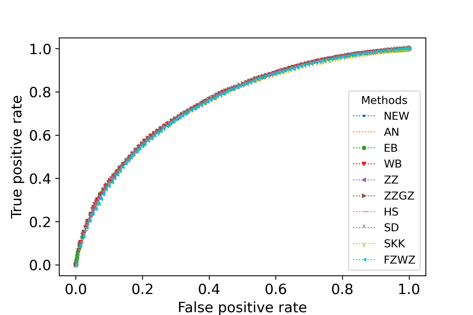
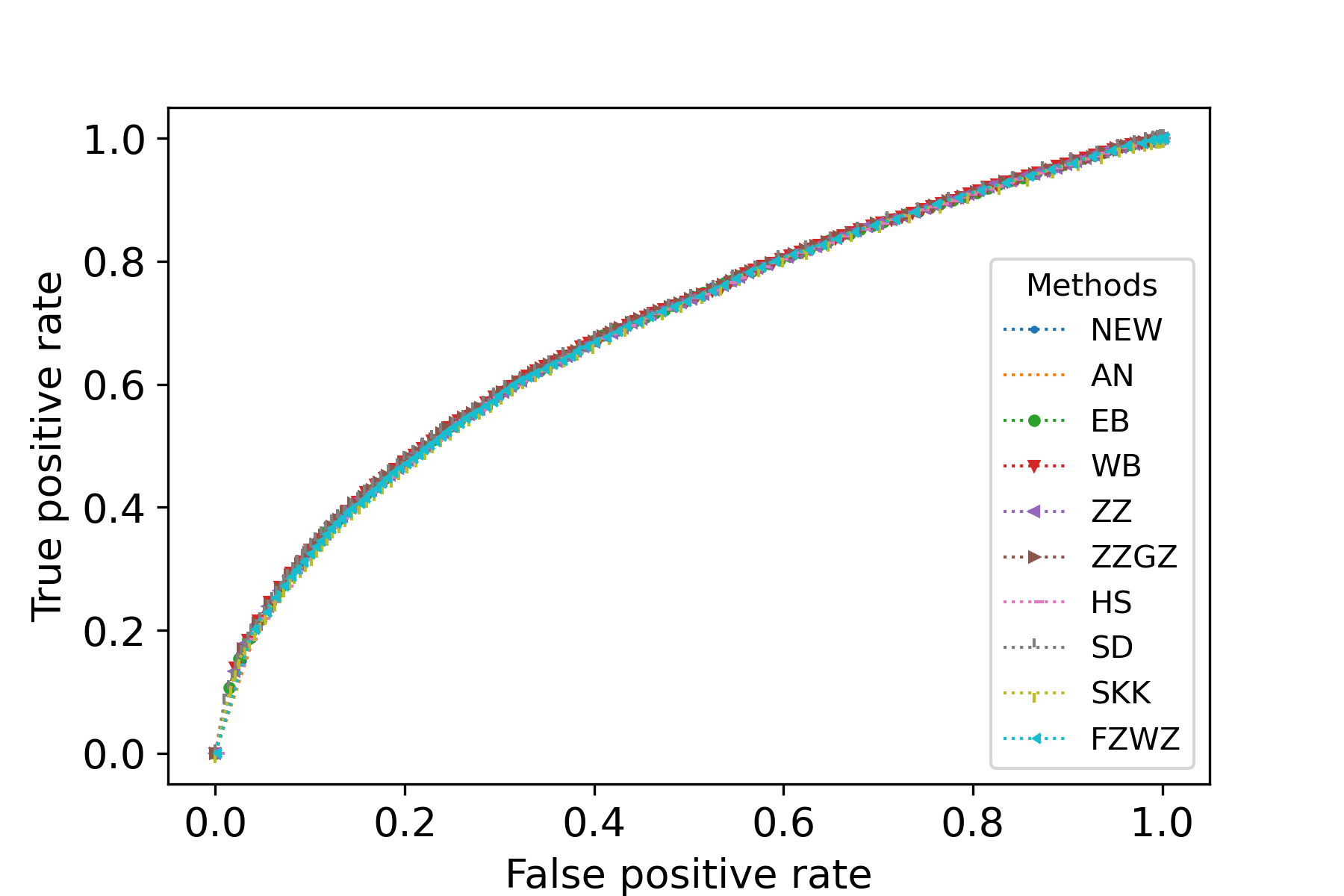
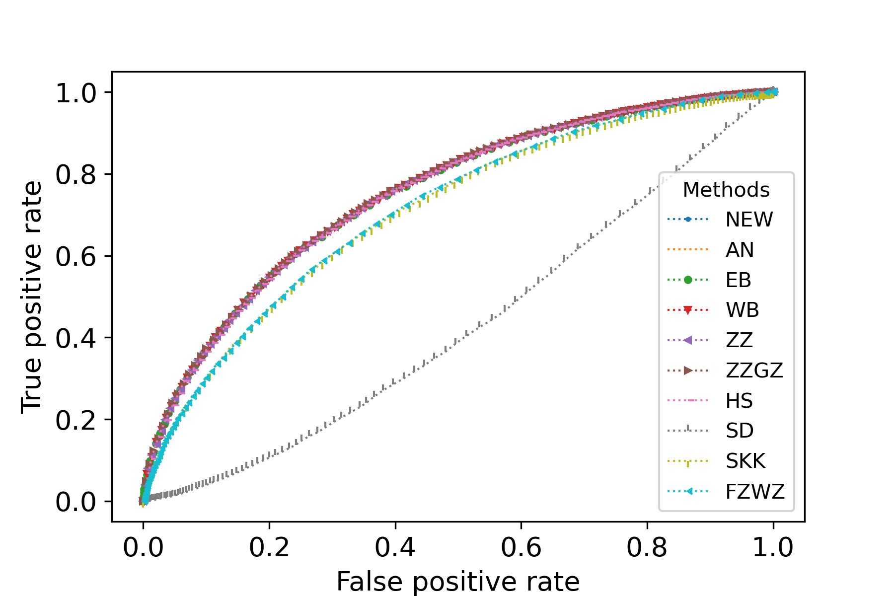
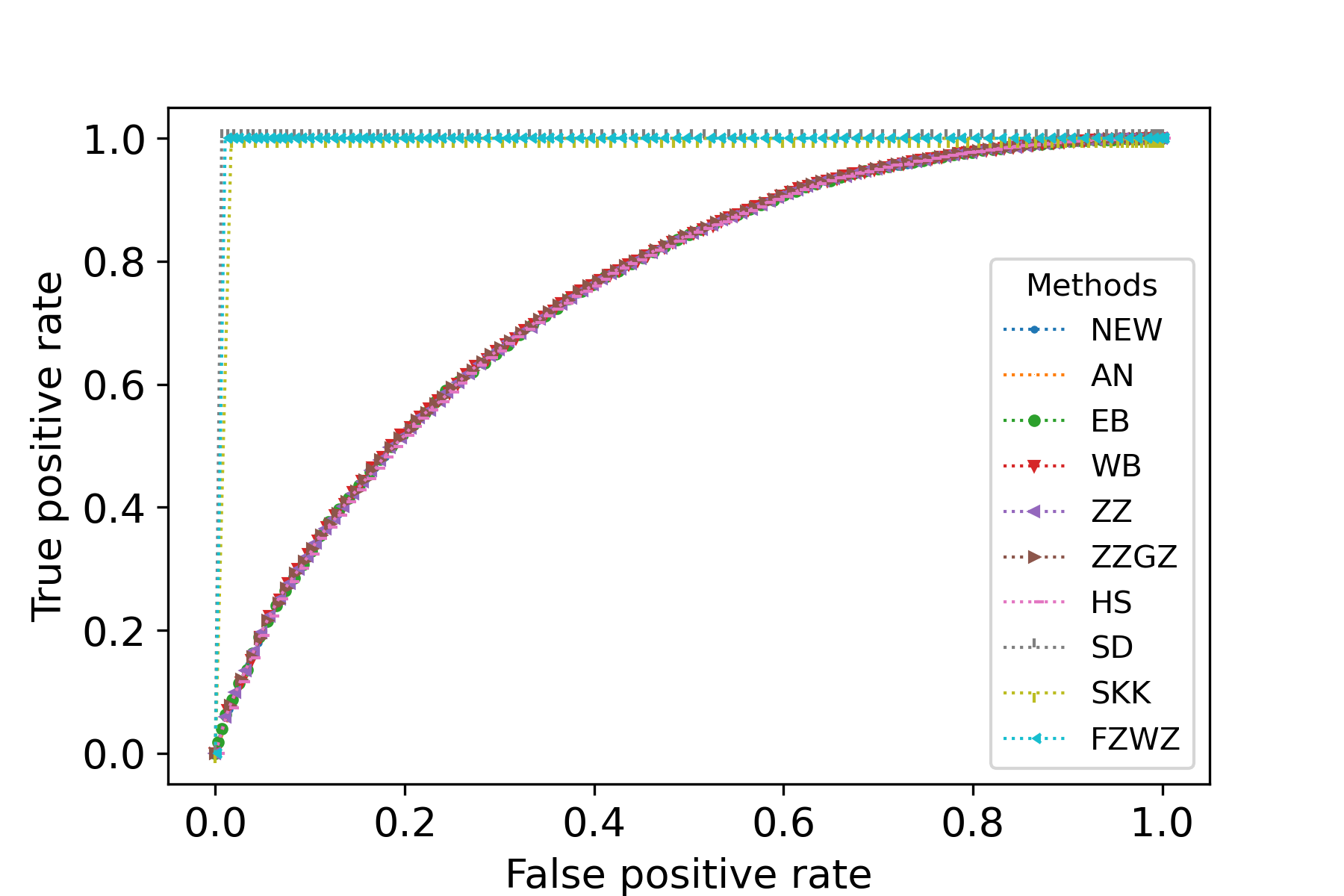
Now we consider the empirical powers of various test procedures. In view of the expression of the asymptotic power given in Corollary 2, we define the signal-to-noise ratio β=μ1μ22/{2tr(𝚿n2)}1/2\beta=\|\mu_{1}-\mu_{2}\|^{2}/\{2\operatorname{tr}(\bm{\Psi}_{n}^{2})\}^{1/2}. We take μ1=𝟎p\mu_{1}=\mathbf{0}_{p} and μ2=c𝟏p\mu_{2}=c\mathbf{1}_{p} where cc is chosen such that β\beta reaches given values of signal-to-noise ratio. Table 2 lists the empirical powers of various test procedures when p=300p=300. It can be seen that for Model IV where the variables have different variance scale, the scalar-invariant tests have better performance than other tests. However, for Model III where 𝚺k,1,,𝚺k,nk\bm{\Sigma}_{k,1},\ldots,\bm{\Sigma}_{k,n_{k}} are not identical and the observations have skewed distributions, the scalar-invariant tests have relatively low powers. The proposed test procedure has a reasonable power behavior among the test procedures based on 𝐗¯1𝐗¯22\|\bar{\mathbf{X}}_{1}-\bar{\mathbf{X}}_{2}\|^{2} or TCQ(𝐗1,𝐗2)T_{\mathrm{CQ}}(\mathbf{X}_{1},\mathbf{X}_{2}). We have seen that some competing tests do not have a good control of test level. To get rid of the effect of distorted test level on the power, we present the receiver operating characteristic curves of the test procedures in Section S.1. It shows that for a given test level, all test procedures based on 𝐗¯1𝐗¯22\|\bar{\mathbf{X}}_{1}-\bar{\mathbf{X}}_{2}\|^{2} or TCQ(𝐗1,𝐗2)T_{\mathrm{CQ}}(\mathbf{X}_{1},\mathbf{X}_{2}) have quite similar power behavior. In summary, the proposed test procedure has promising performance of empirical sizes, and has no power loss compared with existing tests based on 𝐗¯1𝐗¯22\|\bar{\mathbf{X}}_{1}-\bar{\mathbf{X}}_{2}\|^{2} or TCQ(𝐗1,𝐗2)T_{\mathrm{CQ}}(\mathbf{X}_{1},\mathbf{X}_{2}).

Table 3: pp-values of test procedures for the real data
NEW CQ EB WB ZZ ZZGZ LOU SD SKK FZWZ
9.99e-4 1.89e-10 9.99e-4 9.99e-4 7.74e-4 7.47e-5 0 0.27 0.18 4.78e-3

NEW, the proposed test procedure; CQ, the test of Chen and Qin, (2010); EB, the empirical bootstrap method based on TCQ(𝐗1,𝐗2)T_{\mathrm{CQ}}(\mathbf{X}_{1},\mathbf{X}_{2}); WB, the wild bootstrap method based on TCQ(𝐗1,𝐗2)T_{\mathrm{CQ}}(\mathbf{X}_{1},\mathbf{X}_{2}); ZZ, the test of Zhang and Zhu, (2021); ZZGZ, the test of Zhang et al., (2021); LOU, the test of Lou, (2020); SD, the test of Srivastava and Du, (2008); SKK, the test of Srivastava et al., (2013); FZWZ, the test of Feng et al., (2015).

5 Real-data example

In this section, we apply the proposed test procedure to the gene expression dataset released by Alon et al., (1999). This dataset consists of the gene expression levels of n1=22n_{1}=22 normal and n2=40n_{2}=40 tumor colon tissue samples. It contains the expression of p=2,000p=2,000 genes with highest minimal intensity across the n=62n=62 tissues. We would like to test if the normal and tumor colon tissue samples have the same average gene expression levels. Table 3 lists the pp-values of various test procedures. With α=0.05\alpha=0.05, all but the test procedures of Srivastava and Du, (2008) and Srivastava et al., (2013) reject the null hypothesis, claiming that the average gene expression levels of normal and tumor colon tissue samples are significantly different.

We would also like to examine the empirical sizes of various test procedures on the gene expression data. To mimick the null distribution of the gene expression data, we generate resampled datasets as follows: the resampled observations {X1,i}i=122\{X_{1,i}^{*}\}_{i=1}^{22} are uniformly sampled from {X1,iX¯1}i=122\{X_{1,i}-\bar{X}_{1}\}_{i=1}^{22} with replacement, and {X2,i}i=140\{X_{2,i}^{*}\}_{i=1}^{40} are uniformly sampled from {X2,iX¯2}i=140\{X_{2,i}-\bar{X}_{2}\}_{i=1}^{40} with replacement. We conduct various test procedures with α=0.05\alpha=0.05 on the resampled observations {Xk,i}\{X_{k,i}^{*}\}. The above procedure is independently replicated for 10,00010,000 times to compute the empirical sizes. The results are listed in Table 4. It can be seen that the test procedures of Srivastava and Du, (2008) and Srivastava et al., (2013) are overly conservative. Hence the pp-values of these two test procedures for gene expression data may not be reliable. The test procedures of Chen and Qin, (2010) and Feng et al., (2015) are a little inflated. In comparison, the remaining test procedures, including the proposed test procedure, have a good control of the test level for the resampled gene expression data. This implies that the pp-value of the proposed test procedure for the gene expression data is reliable.

Table 4: Empirical sizes (multiplied by 100100) of test procedures for the resampled real datasets
NEW CQ EB WB ZZ ZZGZ LOU SD SKK FZWZ
5.43 7.28 5.22 5.84 5.19 5.98 5.71 0.60 0.79 7.03

NEW, the proposed test procedure; CQ, the test of Chen and Qin, (2010); EB, the empirical bootstrap method based on TCQ(𝐗1,𝐗2)T_{\mathrm{CQ}}(\mathbf{X}_{1},\mathbf{X}_{2}); WB, the wild bootstrap method based on TCQ(𝐗1,𝐗2)T_{\mathrm{CQ}}(\mathbf{X}_{1},\mathbf{X}_{2}); ZZ, the test of Zhang and Zhu, (2021); ZZGZ, the test of Zhang et al., (2021); LOU, the test of Lou, (2020); SD, the test of Srivastava and Du, (2008); SKK, the test of Srivastava et al., (2013); FZWZ, the test of Feng et al., (2015).

Acknowledgements

The authors thank the editor, associate editor and three reviewers for their valuable comments and suggestions. This work was supported by Beijing Natural Science Foundation (No Z200001), National Natural Science Foundation of China (No 11971478). Wangli Xu serves as the corresponding author of the present paper.

References

  • Alon et al., (1999) Alon, U., Barkai, N., Notterman, D. A., Gish, K., Ybarra, S., Mack, D., and Levine, A. J. (1999). Broad patterns of gene expression revealed by clustering analysis of tumor and normal colon tissues probed by oligonucleotide arrays. Proceedings of the National Academy of Sciences, 96(12):6745–6750.
  • Bai and Saranadasa, (1996) Bai, Z. and Saranadasa, H. (1996). Effect of high dimension: by an example of a two sample problem. Statistica Sinica, 6(2):311–329.
  • Cai et al., (2013) Cai, T., Liu, W., and Xia, Y. (2013). Two-sample test of high dimensional means under dependence. Journal of the Royal Statistical Society: Series B (Statistical Methodology), 76(2):349–372.
  • Canay et al., (2017) Canay, I. A., Romano, J. P., and Shaikh, A. M. (2017). Randomization tests under an approximate symmetry assumption. Econometrica, 85(3):1013–1030.
  • Chang et al., (2017) Chang, J., Zheng, C., Zhou, W.-X., and Zhou, W. (2017). Simulation-based hypothesis testing of high dimensional means under covariance heterogeneity. Biometrics, 73(4):1300–1310.
  • Chatterjee, (2006) Chatterjee, S. (2006). A generalization of the lindeberg principle. The Annals of Probability, 34(6):2061–2076.
  • Chen and Qin, (2010) Chen, S. X. and Qin, Y. L. (2010). A two-sample test for high-dimensional data with applications to gene-set testing. The Annals of Statistics, 38(2):808–835.
  • Chernozhukov et al., (2013) Chernozhukov, V., Chetverikov, D., and Kato, K. (2013). Gaussian approximations and multiplier bootstrap for maxima of sums of high-dimensional random vectors. The Annals of Statistics, 41(6):2786–2819.
  • Chernozhukov et al., (2017) Chernozhukov, V., Chetverikov, D., and Kato, K. (2017). Central limit theorems and bootstrap in high dimensions. The Annals of Probability, 45(4):2309–2352.
  • Chung and Romano, (2013) Chung, E. and Romano, J. P. (2013). Exact and asymptotically robust permutation tests. The Annals of Statistics, 41(2):484–507.
  • Cohn, (2013) Cohn, D. L. (2013). Measure Theory. Birkhäuser, New York, 2nd edition.
  • de Jong, (1987) de Jong, P. (1987). A central limit theorem for generalized quadratic forms. Probability Theory & Related Fields, 75(2):261–277.
  • Deng and Zhang, (2020) Deng, H. and Zhang, C.-H. (2020). Beyond Gaussian approximation: bootstrap for maxima of sums of independent random vectors. The Annals of Statistics, 48(6):3643–3671.
  • Döbler and Peccati, (2017) Döbler, C. and Peccati, G. (2017). Quantitative de jong theorems in any dimension. Electronic Journal of Probability, 22(0).
  • Dudley, (2002) Dudley, R. M. (2002). Real Analysis and Probability. Cambridge University Press.
  • Fan et al., (2021) Fan, J., Wang, K., Zhong, Y., and Zhu, Z. (2021). Robust high-dimensional factor models with applications to statistical machine learning. Statistical Science, 36(2):303–327.
  • Fang et al., (1990) Fang, K. T., Kotz, S., and Ng, K. W. (1990). Symmetric multivariate and related distributions. Chapman and Hall, Ltd., London.
  • Feng et al., (2015) Feng, L., Zou, C., Wang, Z., and Zhu, L. (2015). Two-sample Behrens-Fisher problem for high-dimensional data. Statistica Sinica, 25(4):1297–1312.
  • Fisher, (1935) Fisher, R. A. (1935). The design of experiments. Oliver and Boyd, Edinburgh, 1 edition.
  • Hemerik and Goeman, (2018) Hemerik, J. and Goeman, J. (2018). Exact testing with random permutations. TEST, 27(4):811–825.
  • Hoeffding, (1952) Hoeffding, W. (1952). The large-sample power of tests based on permutations of observations. The Annals of Mathematical Statistics, 23(2):169–192.
  • Hu and Bai, (2016) Hu, J. and Bai, Z. (2016). A review of 20 years of naive tests of significance for high-dimensional mean vectors and covariance matrices. Science China. Mathematics, 59(12):2281–2300.
  • Kong and Valiant, (2017) Kong, W. and Valiant, G. (2017). Spectrum estimation from samples. The Annals of Statistics, 45(5):2218–2247.
  • Lehmann and Romano, (2005) Lehmann, E. L. and Romano, J. P. (2005). Testing Statistical Hypotheses. Springer, New York, 3rd edition.
  • Linnik, (1966) Linnik, J. V. (1966). Latest investigations on Behrens-Fisher problem. Sankhyā. Series A, 28:15–24.
  • Lou, (2020) Lou, Z. (2020). High Dimensional Inference Based on Quadratic Forms. Thesis (Ph.D.)–The University of Chicago.
  • Mossel et al., (2010) Mossel, E., O’Donnell, R., and Oleszkiewicz, K. (2010). Noise stability of functions with low influences: invariance and optimality. Annals of Mathematics. Second Series, 171(1):295–341.
  • Nourdin et al., (2010) Nourdin, I., Peccati, G., and Reinert, G. (2010). Invariance principles for homogeneous sums: universality of Gaussian Wiener chaos. The Annals of Probability, 38(5):1947–1985.
  • Pollard, (1984) Pollard, D. (1984). Convergence of stochastic processes. Springer, New York, 1st edition.
  • Romano, (1990) Romano, J. P. (1990). On the behavior of randomization tests without a group invariance assumption. Journal of the American Statistical Association, 85(411):686–692.
  • Simon, (2015) Simon, B. (2015). Real analysis. A Comprehensive Course in Analysis, Part 1. American Mathematical Society, Providence, RI. With a 68 page companion booklet.
  • Srivastava and Du, (2008) Srivastava, M. S. and Du, M. (2008). A test for the mean vector with fewer observations than the dimension. Journal of Multivariate Analysis, 99(3):386–402.
  • Srivastava et al., (2013) Srivastava, M. S., Katayama, S., and Kano, Y. (2013). A two sample test in high dimensional data. Journal of Multivariate Analysis, 114(Supplement C):349–358.
  • Tao, (2012) Tao, T. (2012). Topics in random matrix theory, volume 132 of Graduate Studies in Mathematics. American Mathematical Society, Providence, RI.
  • Tropp, (2015) Tropp, J. A. (2015). An introduction to matrix concentration inequalities. Foundations and Trends® in Machine Learning, 8(1-2):1–230.
  • Wang and Xu, (2019) Wang, R. and Xu, X. (2019). A feasible high dimensional randomization test for the mean vector. Journal of Statistical Planning and Inference, 199:160–178.
  • Wu et al., (2018) Wu, W. B., Lou, Z., and Han, Y. (2018). Hypothesis testing for high-dimensional data. In Handbook of big data analytics, pages 203–224.
  • Xu et al., (2019) Xu, M., Zhang, D., and Wu, W. B. (2019). Pearson’s chi-squared statistics: approximation theory and beyond. Biometrika, 106(3):716–723.
  • Xue and Yao, (2020) Xue, K. and Yao, F. (2020). Distribution and correlation-free two-sample test of high-dimensional means. The Annals of Statistics, 48(3):1304–1328.
  • Zhang et al., (2020) Zhang, J.-T., Guo, J., Zhou, B., and Cheng, M.-Y. (2020). A simple two-sample test in high dimensions based on L2L^{2}-norm. Journal of the American Statistical Association, 115(530):1011–1027.
  • Zhang et al., (2021) Zhang, J.-T., Zhou, B., Guo, J., and Zhu, T. (2021). Two-sample Behrens-Fisher problems for high-dimensional data: a normal reference approach. Journal of Statistical Planning and Inference, 213:142–161.
  • Zhang and Zhu, (2021) Zhang, J.-T. and Zhu, T. (2021). A further study on chen-qin’s test for two-sample behrens-fisher problems for high-dimensional data. Department of Statistics and Applied Probability, National University of Singapore.
  • Zhou and Guo, (2017) Zhou, B. and Guo, J. (2017). A note on the unbiased estimator of Σ2\Sigma^{2}. Statistics & Probability Letters, 129:141–146.
  • Zhu, (2005) Zhu, L. (2005). Nonparametric Monte Carlo tests and their applications. Springer, New York.

Appendix S.1 Additional numerical results

In this section, we present additional numerical results. The experimental setting is as described in the main text.

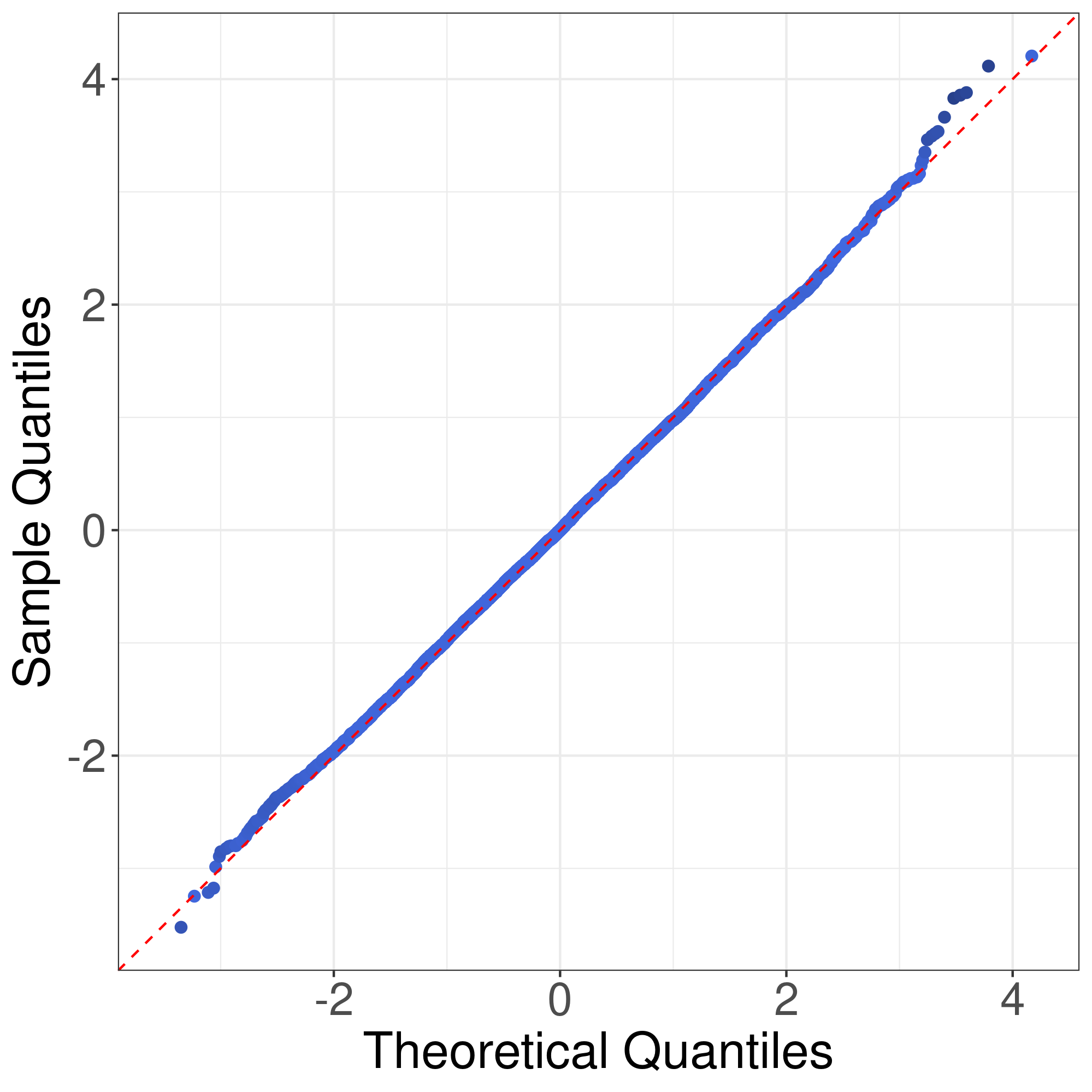
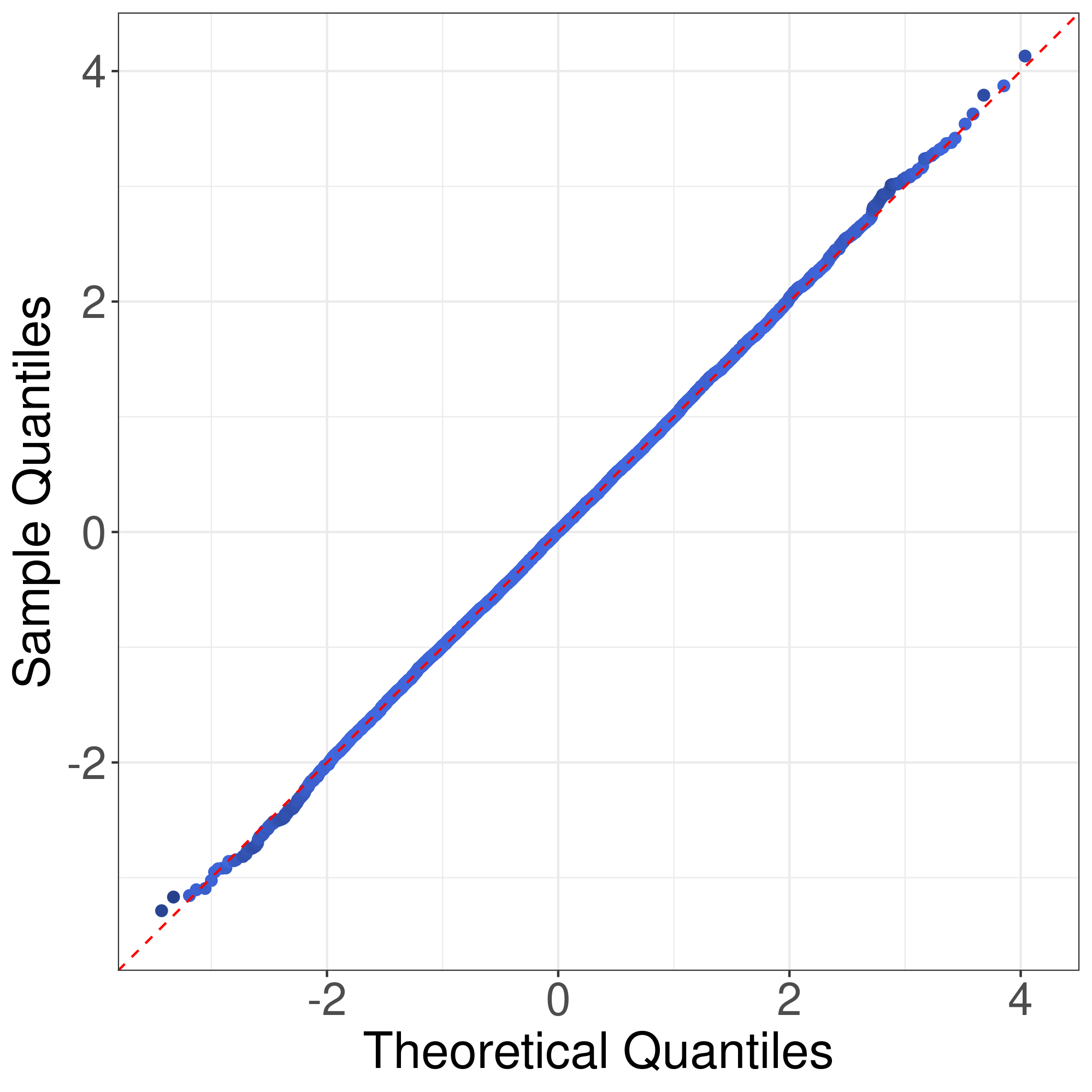
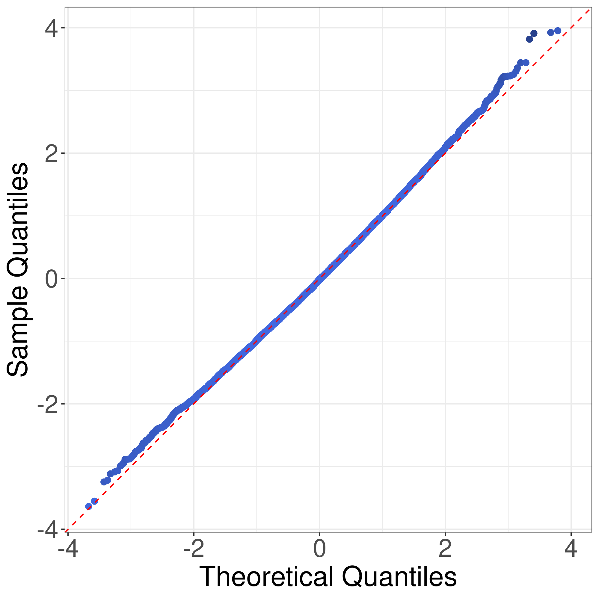
We would like to use quantile-quantile plots to examine the correctness of Theorem 1 and Corollary 1. First we consider the correctness of Theorem 1. Theorem 1 implies that the distribution of TCQ(𝐘1,𝐘2)/σT,nT_{\mathrm{CQ}(\mathbf{Y}_{1},\mathbf{Y}_{2})}/\sigma_{T,n} can be approximated by that of {𝝃p𝚿n𝝃ptr(𝚿n)}/{2tr(𝚿n2)}1/2\{\bm{\xi}_{p}^{\intercal}\bm{\Psi}_{n}\bm{\xi}_{p}-\operatorname{tr}(\bm{\Psi}_{n})\}/\{2\operatorname{tr}(\bm{\Psi}_{n}^{2})\}^{1/2}. Fig. 1 illustrates the plots of the empirical quantiles of TCQ(𝐘1,𝐘2)/σT,nT_{\mathrm{CQ}(\mathbf{Y}_{1},\mathbf{Y}_{2})}/\sigma_{T,n} against that of {𝝃p𝚿n𝝃ptr(𝚿n)}/{2tr(𝚿n2)}1/2\{\bm{\xi}_{p}^{\intercal}\bm{\Psi}_{n}\bm{\xi}_{p}-\operatorname{tr}(\bm{\Psi}_{n})\}/\{2\operatorname{tr}(\bm{\Psi}_{n}^{2})\}^{1/2} under Models I-IV described in the main text with n1=16n_{1}=16, n2=24n_{2}=24, p=300p=300. The empirical quantiles of TCQ(𝐘1,𝐘2)/σT,nT_{\mathrm{CQ}}(\mathbf{Y}_{1},\mathbf{Y}_{2})/\sigma_{T,n} are obtained by 10,00010,000 replications. The results imply that the distribution approximation in Theorem 1 is quite accurate for finite sample size.

(a) Model I
Refer to caption
(b) Model II
Refer to caption
(c) Model III
Refer to caption
(d) Model IV
Refer to caption
Figure 1: Plots of the empirical quantiles of TCQ(𝐘1,𝐘2)/σT,nT_{\mathrm{CQ}(\mathbf{Y}_{1},\mathbf{Y}_{2})}/\sigma_{T,n} against that of (𝝃p𝚿n𝝃ptr(𝚿n))/{2tr(𝚿n2)}1/2(\bm{\xi}_{p}^{\intercal}\bm{\Psi}_{n}\bm{\xi}_{p}-\operatorname{tr}(\bm{\Psi}_{n}))/\{2\operatorname{tr}(\bm{\Psi}_{n}^{2})\}^{1/2}. n1=16n_{1}=16, n2=24n_{2}=24, p=300p=300.
(a) γ=0\gamma=0
Refer to caption
(b) γ=1/p1/2\gamma=1/p^{1/2}
Refer to caption
(c) γ=1/2\gamma=1/2
Refer to caption
(d) γ=1\gamma=1
Refer to caption
Figure 2: Plots of the empirical quantiles of TCQ(𝐘1,𝐘2)/σT,nT_{\mathrm{CQ}}(\mathbf{Y}_{1},\mathbf{Y}_{2})/\sigma_{T,n} against that of the asymptotic distribution in (6). n1=16n_{1}=16, n2=24n_{2}=24, p=300p=300.
(a) Model I
Refer to caption
(b) Model II
Refer to caption
(c) Model III
Refer to caption
(d) Model IV
Refer to caption
Figure 3: Receiver operating characteristic curve of various test procedures. NEW, the proposed test procedure; CQ, the test procedure of Chen and Qin, (2010); EB, the empirical bootstrap method based on TCQ(𝐗1,𝐗2)T_{\mathrm{CQ}}(\mathbf{X}_{1},\mathbf{X}_{2}); WB, the wild bootstrap method based on TCQ(𝐗1,𝐗2)T_{\mathrm{CQ}}(\mathbf{X}_{1},\mathbf{X}_{2}); ZZ, the test procedure of Zhang and Zhu, (2021); ZZGZ, the test procedure of Zhang et al., (2021); LOU, the test procedure of Lou, (2020); SD, the test procedure of Srivastava and Du, (2008); SKK, the test procedure of Srivastava et al., (2013); FZWZ, the test procedure of Feng et al., (2015).

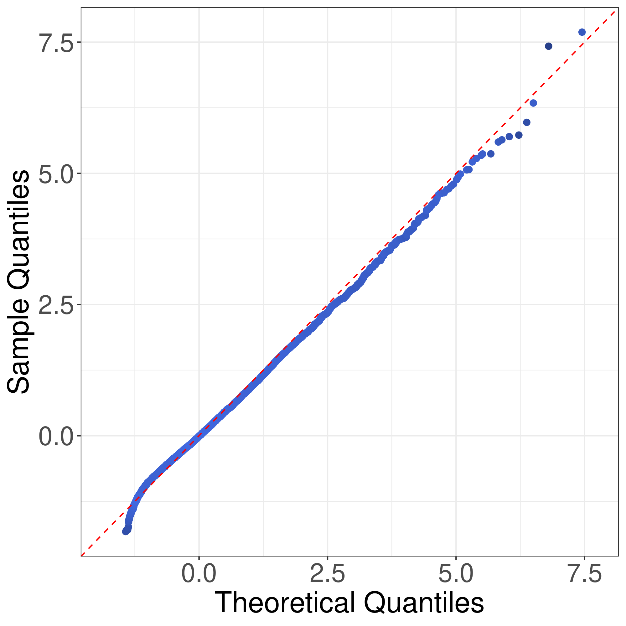
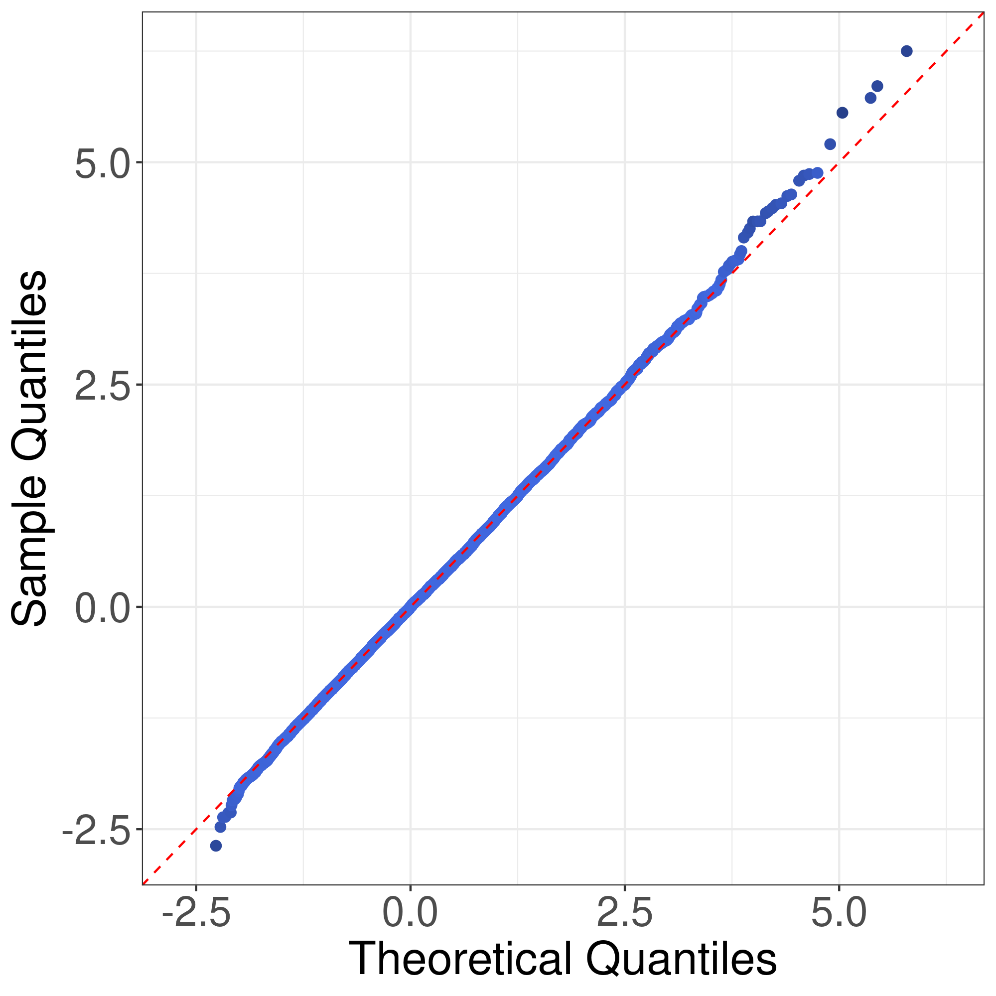
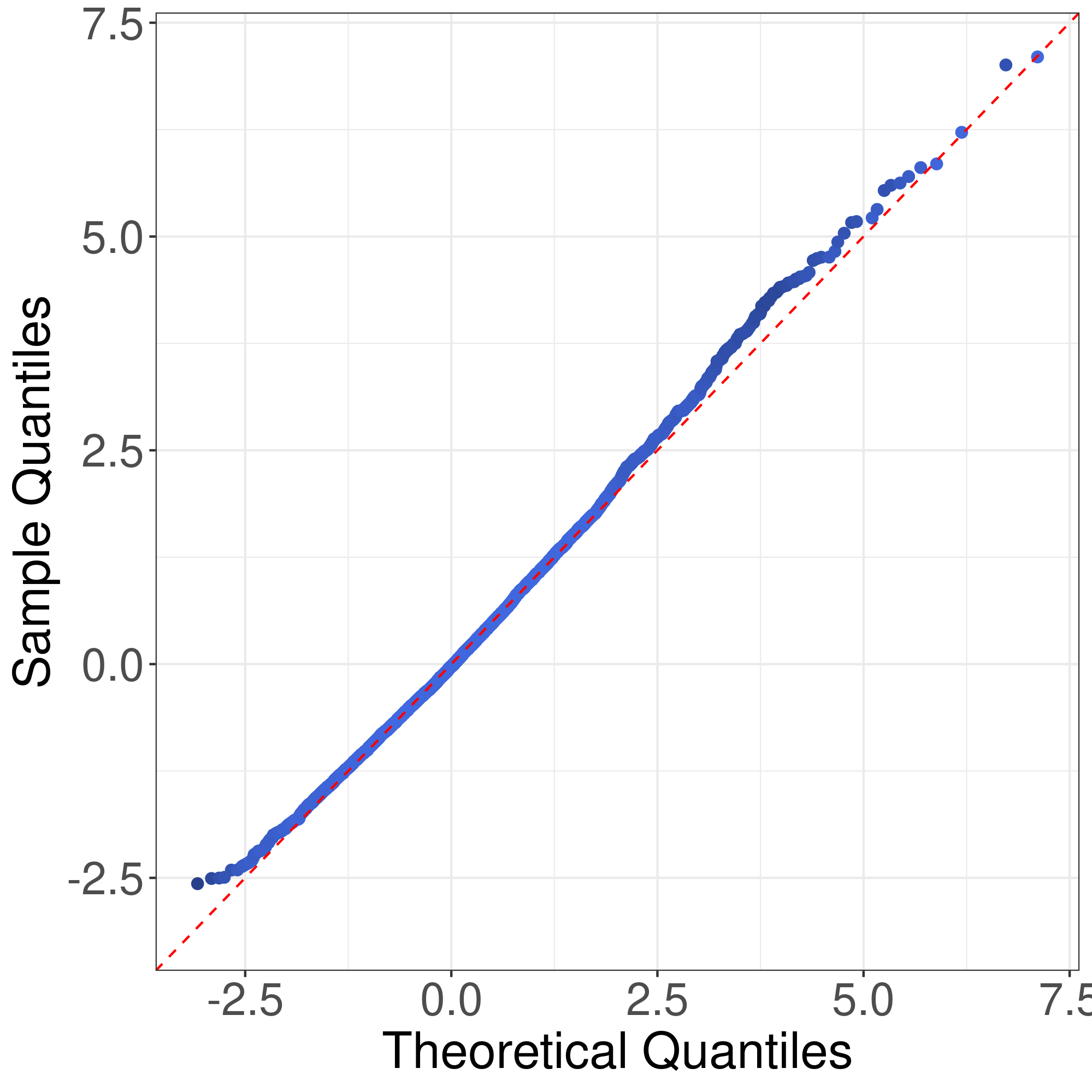
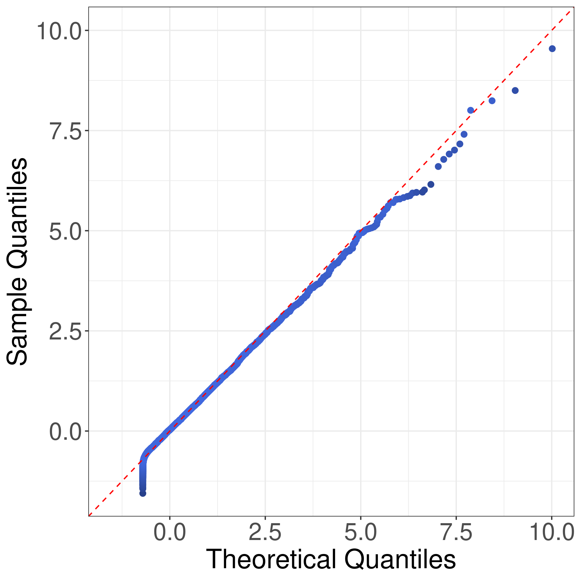
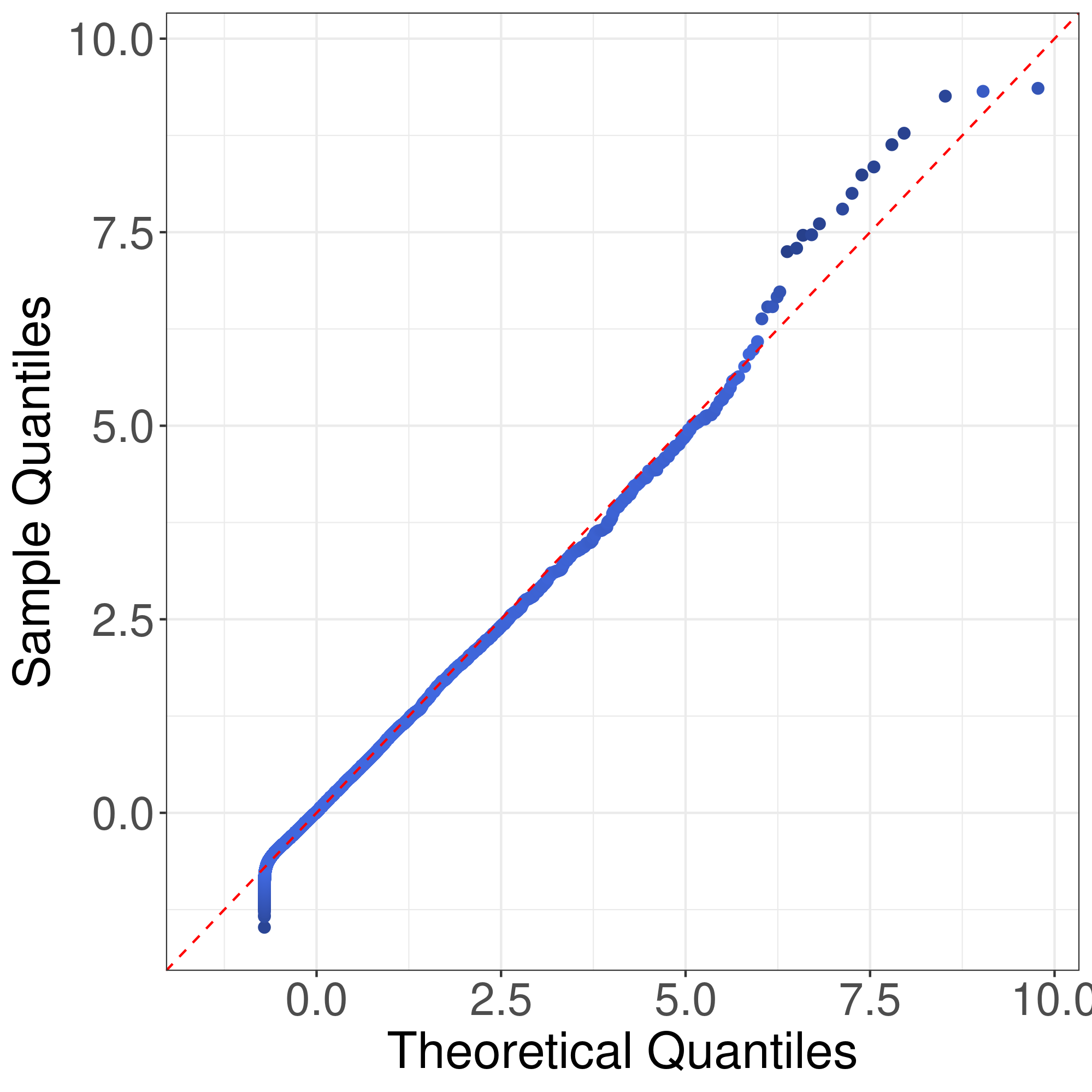
Now we consider the correctness of Corollary 1. Corollary 1 claims that the general asymptotic distributions of TCQ(𝐘1,𝐘2)/σT,nT_{\mathrm{CQ}}(\mathbf{Y}_{1},\mathbf{Y}_{2})/\sigma_{T,n} are weighted sums of independent normal random variable and centered χ2\chi^{2} random variables. In Corollay 1, the parameters {κi}i=1\{\kappa_{i}\}_{i=1}^{\infty} relies on the limits of the eigenvalues of 𝚿n/{tr(𝚿n2)}1/2\bm{\Psi}_{n}/\{\operatorname{tr}(\bm{\Psi}_{n}^{2})\}^{1/2} along a subsequence of {n}\{n\}. To cover different senarios of asymptotic distributions, we consider the following model. Suppose Yk,i𝒩{𝟎p,γ𝟏p𝟏p+(1γ)𝐈p}Y_{k,i}\sim\mathcal{N}\{\mathbf{0}_{p},\gamma\mathbf{1}_{p}\mathbf{1}_{p}^{\intercal}+(1-\gamma)\mathbf{I}_{p}\}, i=1,,nki=1,\ldots,n_{k}, k=1,2k=1,2, where γ[0,1]\gamma\in[0,1]. In this case, the eigenvalues of 𝚿n/{tr(𝚿n2)}1/2\bm{\Psi}_{n}/\{\operatorname{tr}(\bm{\Psi}_{n}^{2})\}^{1/2} are

pγ+1γ{(pγ+1γ)2+(p1)(1γ)2}1/2 and 1γ{(pγ+1γ)2+(p1)(1γ)2}1/2,\displaystyle\frac{p\gamma+1-\gamma}{\{(p\gamma+1-\gamma)^{2}+(p-1)(1-\gamma)^{2}\}^{1/2}}\quad\textrm{ and }\quad\frac{1-\gamma}{\{(p\gamma+1-\gamma)^{2}+(p-1)(1-\gamma)^{2}\}^{1/2}},

with multiplicities 11 and p1p-1, respectively. We assume pp\to\infty as nn\to\infty. We consider four choices of γ\gamma. First, we consider γ=0\gamma=0. In this case, κi=0\kappa_{i}=0, i=1,2,i=1,2,\ldots, and the asymptotic distribution of TCQ(𝐘1,𝐘2)/σT,nT_{\mathrm{CQ}}(\mathbf{Y}_{1},\mathbf{Y}_{2})/\sigma_{T,n} is the standard normal distribution. Second, we consider γ=1/p1/2\gamma=1/p^{1/2}. In this case, κ1=1/2\kappa_{1}=1/\surd 2, and κi=0\kappa_{i}=0, i=2,3,i=2,3,\ldots, and the asymptotic distribution of TCQ(𝐘1,𝐘2)/σT,nT_{\mathrm{CQ}}(\mathbf{Y}_{1},\mathbf{Y}_{2})/\sigma_{T,n} is 𝒩(0,1)/2+{χ2(1)1}/2\mathcal{N}(0,1)/\surd 2+\{\chi^{2}(1)-1\}/2. In the third and fourth cases, we consider γ=1/2\gamma=1/2 and 11, respectively. In these two cases, κ1=1\kappa_{1}=1, and κi=0\kappa_{i}=0, i=2,3,i=2,3,\ldots, and the asymptotic distribution of TCQ(𝐘1,𝐘2)/σT,nT_{\mathrm{CQ}}(\mathbf{Y}_{1},\mathbf{Y}_{2})/\sigma_{T,n} is the standardized χ2\chi^{2} distribution with 11 degree of freedom. Fig. 2 illustrates the plots of the empirical quantiles of TCQ(𝐘1,𝐘2)/σT,nT_{\mathrm{CQ}}(\mathbf{Y}_{1},\mathbf{Y}_{2})/\sigma_{T,n} against that of the asymptotic distribution in (6) for various values of γ\gamma. The empirical quantiles of TCQ(𝐘1,𝐘2)/σT,nT_{\mathrm{CQ}}(\mathbf{Y}_{1},\mathbf{Y}_{2})/\sigma_{T,n} are obtained by 10,00010,000 replications. It can be seen that the distribution of TCQ(𝐘1,𝐘2)/σT,nT_{\mathrm{CQ}}(\mathbf{Y}_{1},\mathbf{Y}_{2})/\sigma_{T,n} can be well approximated by the asymptotic distributions given in Corollary 1. This verifies the conclusion of Corollary 1. We note that the approximation {𝝃p𝚿n𝝃ptr(𝚿n)}/{2tr(𝚿n2)}1/2\{\bm{\xi}_{p}^{\intercal}\bm{\Psi}_{n}\bm{\xi}_{p}-\operatorname{tr}(\bm{\Psi}_{n})\}/\{2\operatorname{tr}(\bm{\Psi}_{n}^{2})\}^{1/2} in Theorem 1 is slightly better than the distribution approximations in Corollary 1. This phenomenon is reasonable since the distributions in Corollary 1 are in fact the asymptotic distributions of {𝝃p𝚿n𝝃ptr(𝚿n)}/{2tr(𝚿n2)}1/2\{\bm{\xi}_{p}^{\intercal}\bm{\Psi}_{n}\bm{\xi}_{p}-\operatorname{tr}(\bm{\Psi}_{n})\}/\{2\operatorname{tr}(\bm{\Psi}_{n}^{2})\}^{1/2} in Theorem 1, and hence may have larger approximation error than {𝝃p𝚿n𝝃ptr(𝚿n)}/{2tr(𝚿n2)}1/2\{\bm{\xi}_{p}^{\intercal}\bm{\Psi}_{n}\bm{\xi}_{p}-\operatorname{tr}(\bm{\Psi}_{n})\}/\{2\operatorname{tr}(\bm{\Psi}_{n}^{2})\}^{1/2}.

We have seen that many competing test procedures do not have a good control of test level. To get rid of the effect of distorted test level, we plot the receiver operating characteristic curve of the test procedures. Fig. 3 illustrates the receiver operating characteristic curve of various test procedures with n1=16n_{1}=16, n2=24n_{2}=24 and p=300p=300. It can be seen that for Models I and II, all test procedures have similar power behavior. For Model III, the scalar-invariant tests are less powerful than other tests. For Model IV, the scalar-invariant tests are more powerful than other tests. These results show that various test procedures based on 𝐗¯1𝐗¯22\|\bar{\mathbf{X}}_{1}-\bar{\mathbf{X}}_{2}\|^{2} or TCQ(𝐗1,𝐗2)T_{\mathrm{CQ}}(\mathbf{X}_{1},\mathbf{X}_{2}) may not have essential difference in power, and their performances are largely driven by the test level.

Appendix S.2 Universality of generalized quadratic forms

In this section, we investigate the universality property of generalized quadratic forms, which is the key tool to study the distributional behavior of the proposed test procedure. The result in this section is also interesting in its own right.

Suppose ξ1,,ξn\xi_{1},\ldots,\xi_{n} are independent random elements taking values in a Polish space 𝒳\mathcal{X}. We consider the generalized quadratic form

W(ξ1,,ξn)=1i<jnwi,j(ξi,ξj),\displaystyle W(\xi_{1},\ldots,\xi_{n})=\sum_{1\leq i<j\leq n}w_{i,j}(\xi_{i},\xi_{j}),

where wi,j(,):𝒳×𝒳w_{i,j}(\cdot,\cdot):\mathcal{X}\times\mathcal{X}\to\mathbb{R} is measurable with respect to the product σ\sigma-algebra on 𝒳×𝒳\mathcal{X}\times\mathcal{X}, 1i<jn1\leq i<j\leq n. The generalized quadratic form includes the statistic TCQ(𝐘1,𝐘2)T_{\mathrm{CQ}}(\mathbf{Y}_{1},\mathbf{Y}_{2}) as a special case. To see this, consider ξi=Y1,i\xi_{i}=Y_{1,i}, i=1,,n1i=1,\ldots,n_{1} and ξj=Y2,jn1\xi_{j}=Y_{2,j-n_{1}}, j=n1+1,,nj=n_{1}+1,\ldots,n. Let

wi,j(ξi,ξj)={2ξiξjn1(n11)for 1i<jn1,2ξiξjn1n2for 1in1 and n1+1jn,2ξiξjn2(n21)for n1+1i<jn.\displaystyle w_{i,j}(\xi_{i},\xi_{j})=\left\{\begin{array}[]{ll}\frac{2\xi_{i}^{\intercal}\xi_{j}}{n_{1}(n_{1}-1)}&\text{for }1\leq i<j\leq n_{1},\\ \frac{-2\xi_{i}^{\intercal}\xi_{j}}{n_{1}n_{2}}&\text{for }1\leq i\leq n_{1}\text{ and }n_{1}+1\leq j\leq n,\\ \frac{2\xi_{i}^{\intercal}\xi_{j}}{n_{2}(n_{2}-1)}&\text{for }n_{1}+1\leq i<j\leq n.\end{array}\right.

In this case, the generalized quadratic form W(ξ1,,ξn)W(\xi_{1},\ldots,\xi_{n}) becomes the statistic TCQ(𝐘1,𝐘2)T_{\mathrm{CQ}}(\mathbf{Y}_{1},\mathbf{Y}_{2}). Similarly, conditioning on 𝐗~1\tilde{\mathbf{X}}_{1} and 𝐗~2\tilde{\mathbf{X}}_{2}, the randomized statistic TCQ(E;𝐗~1,𝐗~2)T_{\mathrm{CQ}}(E;\tilde{\mathbf{X}}_{1},\tilde{\mathbf{X}}_{2}) is a special case of the generalized quadratic form with ξi=ϵ1,i\xi_{i}=\epsilon_{1,i}, i=1,,m1i=1,\ldots,m_{1} and ξj=ϵ2,jm1\xi_{j}=\epsilon_{2,j-m_{1}}, j=m1+1,,m1+m2j=m_{1}+1,\ldots,m_{1}+m_{2}. Hence it is meaningful to investigate the general behavior of the generalized quadratic form.

The asymptotic normality of the generalized quadratic forms was studied by de Jong, (1987) via martingale central limit theorem and by Döbler and Peccati, (2017) via Stein’s method. However, we are interested in the general setting in which W(ξ1,,ξn)W(\xi_{1},\ldots,\xi_{n}) may not be asymptotically normally distributed. Therefore, compared with the asymptotic normality, we are more interested in the universality property of W(ξ1,,ξn)W(\xi_{1},\ldots,\xi_{n}); i.e., the distributional behavior of W(ξ1,,ξn)W(\xi_{1},\ldots,\xi_{n}) does not rely on the particular distribution of ξ1,,ξn\xi_{1},\ldots,\xi_{n} asymptotically. In this regard, many achievements have been made for the universality of W(ξ1,,ξn)W(\xi_{1},\ldots,\xi_{n}) for special form of wi,j(ξi,ξj)w_{i,j}(\xi_{i},\xi_{j}); see, e.g., Mossel et al., (2010), Nourdin et al., (2010), Xu et al., (2019) and the references therein. However, these results can not be used to deal with TCQ(𝐘1,𝐘2)T_{\mathrm{CQ}}(\mathbf{Y}_{1},\mathbf{Y}_{2}) in our setting. In fact, the results in Mossel et al., (2010) and Nourdin et al., (2010) can not be readily applied to TCQ(𝐘1,𝐘2)T_{\mathrm{CQ}}(\mathbf{Y}_{1},\mathbf{Y}_{2}) while the result in Xu et al., (2019) can only be applied to identically distributed observations. To the best of our knowledge, the universality of the generalized quadratic forms was never considered in the literature. We shall derive a universality property of the generalized quadratic forms using Lindeberg principle, an old and powerful technique; see, e.g., Chatterjee, (2006), Mossel et al., (2010) for more about Lindeberg principle.

Assumption S.1.

Suppose ξ1,,ξn\xi_{1},\ldots,\xi_{n} are independent random elements taking values in a Polish space 𝒳\mathcal{X}. Assume the following conditions hold for all 1i<jn1\leq i<j\leq n:

  1. (a)

    E{wi,j(ξi,ξj)4}<\operatorname{E}\{w_{i,j}(\xi_{i},\xi_{j})^{4}\}<\infty.

  2. (b)

    For all 𝐚𝒳\mathbf{a}\in\mathcal{X}, E{wi,j(ξi,𝐚)}=E{wi,j(𝐚,ξj)}=0\operatorname{E}\left\{w_{i,j}(\xi_{i},\mathbf{a})\right\}=\operatorname{E}\left\{w_{i,j}(\mathbf{a},\xi_{j})\right\}=0.

Define σi,j2=E{wi,j(ξi,ξj)2}\sigma_{i,j}^{2}=\operatorname{E}\{w_{i,j}(\xi_{i},\xi_{j})^{2}\}. Under Assumption S.1, we have E{W(ξ1,,ξn)}=0\operatorname{E}\{W(\xi_{1},\ldots,\xi_{n})\}=0 and var{W(ξ1,,ξn)}=1=1nj=i+1nσi,j2\operatorname{var}\{W(\xi_{1},\ldots,\xi_{n})\}=\sum_{1=1}^{n}\sum_{j=i+1}^{n}\sigma_{i,j}^{2}. We would like to give explicit bound for the difference between the distributions of W(ξ1,,ξn)W(\xi_{1},\ldots,\xi_{n}) and W(η1,,ηn)W(\eta_{1},\ldots,\eta_{n}) for a general class of random vectors η1,,ηn\eta_{1},\ldots,\eta_{n}. We impose the following conditions on η1,,ηn\eta_{1},\ldots,\eta_{n}.

Assumption S.2.

Suppose η1,,ηn\eta_{1},\ldots,\eta_{n} are independent random elements taking values in 𝒳\mathcal{X} and are independent of ξ1,,ξn\xi_{1},\ldots,\xi_{n}. Assume the following conditions hold for all 1i<jn1\leq i<j\leq n:

  1. (a)

    E{wi,j(ξi,ηj)4}<\operatorname{E}\{w_{i,j}(\xi_{i},\eta_{j})^{4}\}<\infty, E{wi,j(ηi,ξj)4}<\operatorname{E}\{w_{i,j}(\eta_{i},\xi_{j})^{4}\}<\infty and E{wi,j(ηi,ηj)4}<\operatorname{E}\{w_{i,j}(\eta_{i},\eta_{j})^{4}\}<\infty.

  2. (b)

    For all 𝐚𝒳\mathbf{a}\in\mathcal{X}, E{wi,j(ηi,𝐚)}=E{wi,j(𝐚,ηj)}=0\operatorname{E}\{w_{i,j}(\eta_{i},\mathbf{a})\}=\operatorname{E}\{w_{i,j}(\mathbf{a},\eta_{j})\}=0.

  3. (c)

    For any 𝐚,𝐛𝒳\mathbf{a},\mathbf{b}\in\mathcal{X},

    E{wi,k(𝐚,ξk)wj,k(𝐛,ξk)}=E{wi,k(𝐚,ηk)wj,k(𝐛,ηk)},for1ij<kn,\displaystyle\operatorname{E}\{w_{i,k}(\mathbf{a},\xi_{k})w_{j,k}(\mathbf{b},\xi_{k})\}=\operatorname{E}\{w_{i,k}(\mathbf{a},\eta_{k})w_{j,k}(\mathbf{b},\eta_{k})\},\quad\mathrm{for}\quad 1\leq i\leq j<k\leq n,
    E{wi,j(𝐚,ξj)wj,k(ξj,𝐛)}=E{wi,j(𝐚,ηj)wj,k(ηj,𝐛)},for1i<j<kn,\displaystyle\operatorname{E}\{w_{i,j}(\mathbf{a},\xi_{j})w_{j,k}(\xi_{j},\mathbf{b})\}=\operatorname{E}\{w_{i,j}(\mathbf{a},\eta_{j})w_{j,k}(\eta_{j},\mathbf{b})\},\quad\mathrm{for}\quad 1\leq i<j<k\leq n,
    E{wi,j(ξi,𝐚)wi,k(ξi,𝐛)}=E{wi,j(ηi,𝐚)wi,k(ηi,𝐛)},for1i<jkn.\displaystyle\operatorname{E}\{w_{i,j}(\xi_{i},\mathbf{a})w_{i,k}(\xi_{i},\mathbf{b})\}=\operatorname{E}\{w_{i,j}(\eta_{i},\mathbf{a})w_{i,k}(\eta_{i},\mathbf{b})\},\quad\mathrm{for}\quad 1\leq i<j\leq k\leq n.

We claim that under Assumptions S.1 and S.2, there exists a nonnegative CC (which possibly depends on nn) such that for all 1i<jn1\leq i<j\leq n,

max[E{wi,j(ξi,ξj)4},E{wi,j(ξi,ηj)4},E{wi,j(ηi,ξj)4},E{wi,j(ηi,ηj)4}]Cσi,j4.\displaystyle\max\left[\operatorname{E}\{w_{i,j}(\xi_{i},\xi_{j})^{4}\},\operatorname{E}\{w_{i,j}(\xi_{i},\eta_{j})^{4}\},\operatorname{E}\{w_{i,j}(\eta_{i},\xi_{j})^{4}\},\operatorname{E}\{w_{i,j}(\eta_{i},\eta_{j})^{4}\}\right]\leq C\sigma_{i,j}^{4}. (S.1)

In fact, by Assumption S.1, (a) and Assumption S.2, (a), the left hand side of (S.1) is finite. Also, if σi,j4=0\sigma_{i,j}^{4}=0, that is, E{wi,j(ξi,ξj)2}=0\operatorname{E}\{w_{i,j}(\xi_{i},\xi_{j})^{2}\}=0, then from (c) of Assumption S.2,

0=E{wi,j(ξi,ξj)2}=E{wi,j(ξi,ηj)2}=E{wi,j(ηi,ξj)2}=E{wi,j(ηi,ηj)2}.\displaystyle 0=\operatorname{E}\{w_{i,j}(\xi_{i},\xi_{j})^{2}\}=\operatorname{E}\{w_{i,j}(\xi_{i},\eta_{j})^{2}\}=\operatorname{E}\{w_{i,j}(\eta_{i},\xi_{j})^{2}\}=\operatorname{E}\{w_{i,j}(\eta_{i},\eta_{j})^{2}\}.

It follows that wi,j(ξi,ξj)=wi,j(ξi,ηj)=wi,j(ηi,ξj)=wi,j(ηi,ηj)=0w_{i,j}(\xi_{i},\xi_{j})=w_{i,j}(\xi_{i},\eta_{j})=w_{i,j}(\eta_{i},\xi_{j})=w_{i,j}(\eta_{i},\eta_{j})=0 almost surely. In this case, the left hand side of (S.1) is also 0. Hence our claim is valid. Let ρn\rho_{n} denote the minimum nonnegative CC such that (S.1) holds for all 1i<jn1\leq i<j\leq n, It will turn out that the difference between the distributions of W(ξ1,,ξn)W(\xi_{1},\ldots,\xi_{n}) and W(η1,,ηn)W(\eta_{1},\ldots,\eta_{n}) relies on ρn\rho_{n}.

As in Mossel et al., (2010), we define the influence of ξi\xi_{i} on W(ξ1,,ξn)W(\xi_{1},\ldots,\xi_{n}) as

Infi=E{var(W(ξ1,,ξn)ξ1,,ξi1,ξi+1,,ξn)}.\displaystyle\mathrm{Inf}_{i}=\operatorname{E}\left\{\operatorname{var}(W(\xi_{1},\ldots,\xi_{n})\mid\xi_{1},\ldots,\xi_{i-1},\xi_{i+1},\ldots,\xi_{n})\right\}.

It can be seen that Infi=j=1i1σj,i2+j=i+1nσi,j2\mathrm{Inf}_{i}=\sum_{j=1}^{i-1}\sigma_{j,i}^{2}+\sum_{j=i+1}^{n}\sigma_{i,j}^{2}.

The following theorem provides a universality property of W(ξ1,,ξn)W(\xi_{1},\ldots,\xi_{n}).

Theorem S.1.

Under Assumptions S.1 and S.2, we have

{W(ξ1,,ξn)}{W(η1,,ηn)}3ρn3/431/4i=1nInfi3/2.\displaystyle\left\|\mathcal{L}\{W(\xi_{1},\ldots,\xi_{n})\}-\mathcal{L}\{W(\eta_{1},\ldots,\eta_{n})\}\right\|_{3}\leq\frac{\rho_{n}^{3/4}}{3^{1/4}}\sum_{i=1}^{n}\mathrm{Inf}_{i}^{3/2}.

From Theorem S.1, the distance between W(ξ1,,ξn)W(\xi_{1},\ldots,\xi_{n}) and W(η1,,ηn)W(\eta_{1},\ldots,\eta_{n}) is bounded by a function of ρn\rho_{n} and the influences. Suppose as nn\to\infty, ρn\rho_{n} is bounded and i=1nInfi3/2\sum_{i=1}^{n}\mathrm{Inf}_{i}^{3/2} tends to 0. Then Theorem S.1 implies that W(ξ1,,ξn)W(\xi_{1},\ldots,\xi_{n}) and W(η1,,ηn)W(\eta_{1},\ldots,\eta_{n}) share the same possible asymptotic dsitribution. That is, the distribution of W(ξ1,,ξn)W(\xi_{1},\ldots,\xi_{n}) enjoys a universality property. In the proof of Theorem 1 and Theorem 2, we apply Theorem S.1 to TCQ(𝐘1,𝐘2)T_{\mathrm{CQ}}(\mathbf{Y}_{1},\mathbf{Y}_{2}) and TCQ(E;𝐗~1,𝐗~2)T_{\mathrm{CQ}}(E;\tilde{\mathbf{X}}_{1},\tilde{\mathbf{X}}_{2}), respectively, and consider normally distributed ηi\eta_{i}, i=1,,ni=1,\ldots,n. With this technique, the distributional behaviors of TCQ(𝐘1,𝐘2)T_{\mathrm{CQ}}(\mathbf{Y}_{1},\mathbf{Y}_{2}) and TCQ(E;𝐗~1,𝐗~2)T_{\mathrm{CQ}}(E;\tilde{\mathbf{X}}_{1},\tilde{\mathbf{X}}_{2}) are reduced to the circumstances where the observations are normally distributed.

of Theorem S.1.

For k=1,,n+1k=1,\ldots,n+1, define

Wk=\displaystyle W_{k}= W(η1,,ηk1,ξk,,ξn).\displaystyle W(\eta_{1},\ldots,\eta_{k-1},\xi_{k},\dots,\xi_{n}).

Then W1=W(ξ1,,ξn)W_{1}=W(\xi_{1},\ldots,\xi_{n}) and Wn+1=W(η1,,ηn)W_{n+1}=W(\eta_{1},\ldots,\eta_{n}). Fix an f𝒞b3()f\in\mathscr{C}_{b}^{3}(\mathbb{R}). We have

|Ef(W(ξ1,,ξn))Ef(W(η1,,ηn))|\displaystyle\left|\operatorname{E}f(W(\xi_{1},\ldots,\xi_{n}))-\operatorname{E}f(W(\eta_{1},\ldots,\eta_{n}))\right|\leq k=1n|E{f(Wk)f(Wk+1)}|.\displaystyle\sum_{k=1}^{n}\left|\operatorname{E}\left\{f(W_{k})-f(W_{k+1})\right\}\right|. (S.2)

Define

Wk,0=1i<jk1wi,j(ηi,ηj)+k+1i<jnwi,j(ξi,ξj)+1ik1k+1jnwi,j(ηi,ξj).\displaystyle W_{k,0}=\sum_{1\leq i<j\leq k-1}w_{i,j}(\eta_{i},\eta_{j})+\sum_{k+1\leq i<j\leq n}w_{i,j}(\xi_{i},\xi_{j})+\sum_{1\leq i\leq k-1}\sum_{k+1\leq j\leq n}w_{i,j}(\eta_{i},\xi_{j}).

Note that Wk,0W_{k,0} only relies on η1,,ηk1,ξk+1,,ξn\eta_{1},\ldots,\eta_{k-1},\xi_{k+1},\ldots,\xi_{n}. It can be seen that

Wk=\displaystyle W_{k}= Wk,0+i=1k1wi,k(ηi,ξk)+j=k+1nwk,j(ξk,ξj),\displaystyle W_{k,0}+\sum_{i=1}^{k-1}w_{i,k}(\eta_{i},\xi_{k})+\sum_{j=k+1}^{n}w_{k,j}(\xi_{k},\xi_{j}),
Wk+1=\displaystyle W_{k+1}= Wk,0+i=1k1wi,k(ηi,ηk)+j=k+1nwk,j(ηk,ξj).\displaystyle W_{k,0}+\sum_{i=1}^{k-1}w_{i,k}(\eta_{i},\eta_{k})+\sum_{j=k+1}^{n}w_{k,j}(\eta_{k},\xi_{j}).

From Taylor’s theorem,

|f(Wk)f(Wk,0)i=121i!(WkWk,0)if(i)(Wk,0)|supx|f(3)(x)|6|WkWk,0|3,\displaystyle\left|f(W_{k})-f(W_{k,0})-\sum_{i=1}^{2}\frac{1}{i!}(W_{k}-W_{k,0})^{i}f^{(i)}(W_{k,0})\right|\leq\frac{\sup_{x\in\mathbb{R}}|f^{(3)}(x)|}{6}\left|W_{k}-W_{k,0}\right|^{3}, (S.3)
|f(Wk+1)f(Wk,0)i=121i!(Wk+1Wk,0)if(i)(Wk,0)|supx|f(3)(x)|6|Wk+1Wk,0|3.\displaystyle\left|f(W_{k+1})-f(W_{k,0})-\sum_{i=1}^{2}\frac{1}{i!}(W_{k+1}-W_{k,0})^{i}f^{(i)}(W_{k,0})\right|\leq\frac{\sup_{x\in\mathbb{R}}|f^{(3)}(x)|}{6}\left|W_{k+1}-W_{k,0}\right|^{3}. (S.4)

Now we show that

E{i=121i!(WkWk,0)if(i)(Wk,0)}=E{i=121i!(Wk+1Wk,0)if(i)(Wk,0)}.\displaystyle\operatorname{E}\left\{\sum_{i=1}^{2}\frac{1}{i!}(W_{k}-W_{k,0})^{i}f^{(i)}(W_{k,0})\right\}=\operatorname{E}\left\{\sum_{i=1}^{2}\frac{1}{i!}(W_{k+1}-W_{k,0})^{i}f^{(i)}(W_{k,0})\right\}. (S.5)

By conditioning on η1,,ηk1,ξk+1,,ξn\eta_{1},\ldots,\eta_{k-1},\xi_{k+1},\ldots,\xi_{n}, it can be seen that (S.5) holds provided that for k=1,,nk=1,\ldots,n and =1,2\ell=1,2,

E{(WkWk,0)η1,,ηk1,ξk+1,,ξn}=E{(Wk+1Wk,0)η1,,ηk1,ξk+1,,ξn}.\displaystyle\operatorname{E}\{(W_{k}-W_{k,0})^{\ell}\mid\eta_{1},\ldots,\eta_{k-1},\xi_{k+1},\ldots,\xi_{n}\}=\operatorname{E}\{(W_{k+1}-W_{k,0})^{\ell}\mid\eta_{1},\ldots,\eta_{k-1},\xi_{k+1},\ldots,\xi_{n}\}.

For the case of =1\ell=1, we have

E{WkWk,0η1,,ηk1,ξk+1,,ξn}=i=1k1E{wi,k(ηi,ξk)ηi}+j=k+1nE{wk,j(ξk,ξj)ξj},\displaystyle\operatorname{E}\{W_{k}-W_{k,0}\mid\eta_{1},\ldots,\eta_{k-1},\xi_{k+1},\ldots,\xi_{n}\}=\sum_{i=1}^{k-1}\operatorname{E}\{w_{i,k}(\eta_{i},\xi_{k})\mid\eta_{i}\}+\sum_{j=k+1}^{n}\operatorname{E}\{w_{k,j}(\xi_{k},\xi_{j})\mid\xi_{j}\},

which equals 0 by (b) of Assumption S.1. Similarly, we have

E{Wk+1Wk,0η1,,ηk1,ξk+1,,ξn}=0.\displaystyle\operatorname{E}\{W_{k+1}-W_{k,0}\mid\eta_{1},\ldots,\eta_{k-1},\xi_{k+1},\ldots,\xi_{n}\}=0.

Now we deal with the case of =2\ell=2. From (c) of Assumption S.2, we have

E{(WkWk,0)2η1,,ηk1,ξk+1,,ξn}\displaystyle\operatorname{E}\{(W_{k}-W_{k,0})^{2}\mid\eta_{1},\ldots,\eta_{k-1},\xi_{k+1},\ldots,\xi_{n}\}
=\displaystyle= i1=1k1i2=1k1E{wi1,k(ηi1,ξk)wi2,k(ηi2,ξk)ηi1,ηi2}+j1=k+1nj2=k+1nE{wk,j1(ξk,ξj1)wk,j2(ξk,ξj2)ξj1,ξj2}\displaystyle\sum_{i_{1}=1}^{k-1}\sum_{i_{2}=1}^{k-1}\operatorname{E}\{w_{i_{1},k}(\eta_{i_{1}},\xi_{k})w_{i_{2},k}(\eta_{i_{2}},\xi_{k})\mid\eta_{i_{1}},\eta_{i_{2}}\}+\sum_{j_{1}=k+1}^{n}\sum_{j_{2}=k+1}^{n}\operatorname{E}\{w_{k,j_{1}}(\xi_{k},\xi_{j_{1}})w_{k,j_{2}}(\xi_{k},\xi_{j_{2}})\mid\xi_{j_{1}},\xi_{j_{2}}\}
+2i=1k1j=k+1nE{wi,k(ηi,ξk)wk,j(ξk,ξj)ηi,ξj}\displaystyle+2\sum_{i=1}^{k-1}\sum_{j=k+1}^{n}\operatorname{E}\{w_{i,k}(\eta_{i},\xi_{k})w_{k,j}(\xi_{k},\xi_{j})\mid\eta_{i},\xi_{j}\}
=\displaystyle= i1=1k1i2=1k1E{wi1,k(ηi1,ηk)wi2,k(ηi2,ηk)ηi1,ηi2}+j1=k+1nj2=k+1nE{wk,j1(ηk,ξj1)wk,j2(ηk,ξj2)ξj1,ξj2}\displaystyle\sum_{i_{1}=1}^{k-1}\sum_{i_{2}=1}^{k-1}\operatorname{E}\{w_{i_{1},k}(\eta_{i_{1}},\eta_{k})w_{i_{2},k}(\eta_{i_{2}},\eta_{k})\mid\eta_{i_{1}},\eta_{i_{2}}\}+\sum_{j_{1}=k+1}^{n}\sum_{j_{2}=k+1}^{n}\operatorname{E}\{w_{k,j_{1}}(\eta_{k},\xi_{j_{1}})w_{k,j_{2}}(\eta_{k},\xi_{j_{2}})\mid\xi_{j_{1}},\xi_{j_{2}}\}
+2i=1k1j=k+1nE{wi,k(ηi,ηk)wk,j(ηk,ξj)ηi,ξj}\displaystyle+2\sum_{i=1}^{k-1}\sum_{j=k+1}^{n}\operatorname{E}\{w_{i,k}(\eta_{i},\eta_{k})w_{k,j}(\eta_{k},\xi_{j})\mid\eta_{i},\xi_{j}\}
=\displaystyle= E{(Wk+1Wk,0)2η1,,ηk1,ξk+1,,ξn}.\displaystyle\operatorname{E}\{(W_{k+1}-W_{k,0})^{2}\mid\eta_{1},\ldots,\eta_{k-1},\xi_{k+1},\ldots,\xi_{n}\}.

Therefore, (S.5) holds. It follows from (S.3), (S.4) and (S.5) that

|Ef(Wk+1)Ef(Wk)|\displaystyle\left|\operatorname{E}f(W_{k+1})-\operatorname{E}f(W_{k})\right|\leq supx|f(3)(x)|6(E|WkWk,0|3+E|Wk+1Wk,0|3)\displaystyle\frac{\sup_{x\in\mathbb{R}}|f^{(3)}(x)|}{6}\left(\operatorname{E}\left|W_{k}-W_{k,0}\right|^{3}+\operatorname{E}\left|W_{k+1}-W_{k,0}\right|^{3}\right)
\displaystyle\leq supx|f(3)(x)|6[[E{(WkWk,0)4}]3/4+[E{(Wk+1Wk,0)4}]3/4].\displaystyle\frac{\sup_{x\in\mathbb{R}}|f^{(3)}(x)|}{6}\left[\left[\operatorname{E}\left\{\left(W_{k}-W_{k,0}\right)^{4}\right\}\right]^{3/4}+\left[\operatorname{E}\left\{\left(W_{k+1}-W_{k,0}\right)^{4}\right\}\right]^{3/4}\right].

Combining (S.2) and the above inequality leads to

|Ef(W(η1,,ηn))Ef(W(ξ1,,ξn))|\displaystyle\left|\operatorname{E}f(W(\eta_{1},\ldots,\eta_{n}))-\operatorname{E}f(W(\xi_{1},\ldots,\xi_{n}))\right|
\displaystyle\leq supx|f(3)(x)|6k=1n[[E{(WkWk,0)4}]3/4+[E{(Wk+1Wk,0)4}]3/4].\displaystyle\frac{\sup_{x\in\mathbb{R}}|f^{(3)}(x)|}{6}\sum_{k=1}^{n}\left[\left[\operatorname{E}\left\{\left(W_{k}-W_{k,0}\right)^{4}\right\}\right]^{3/4}+\left[\operatorname{E}\left\{\left(W_{k+1}-W_{k,0}\right)^{4}\right\}\right]^{3/4}\right].

Now we derive upper bounds for E{(WkWk,0)4}\operatorname{E}\{\left(W_{k}-W_{k,0}\right)^{4}\} and E{(Wk+1Wk,0)4}\operatorname{E}\{\left(W_{k+1}-W_{k,0}\right)^{4}\}. We have

E{(WkWk,0)4}=\displaystyle\operatorname{E}\left\{\left(W_{k}-W_{k,0}\right)^{4}\right\}= E[{i=1k1wi,k(ηi,ξk)}4]+E[{j=k+1nwk,j(ξk,ξj)}4]\displaystyle\operatorname{E}\Big{[}\Big{\{}\sum_{i=1}^{k-1}w_{i,k}(\eta_{i},\xi_{k})\Big{\}}^{4}\Big{]}+\operatorname{E}\Big{[}\Big{\{}\sum_{j=k+1}^{n}w_{k,j}(\xi_{k},\xi_{j})\Big{\}}^{4}\Big{]}
+6E[{i=1k1wi,k(ηi,ξk)}2{j=k+1nwk,j(ξk,ξj)}2]\displaystyle+6\operatorname{E}\Big{[}\Big{\{}\sum_{i=1}^{k-1}w_{i,k}(\eta_{i},\xi_{k})\Big{\}}^{2}\Big{\{}\sum_{j=k+1}^{n}w_{k,j}(\xi_{k},\xi_{j})\Big{\}}^{2}\Big{]}
=\displaystyle= i=1k1E{wi,k(ηi,ξk)4}+6i1=1k1i2=i1+1k1E{wi1,k(ηi1,ξk)2wi2,k(ηi2,ξk)2}\displaystyle\sum_{i=1}^{k-1}\operatorname{E}\left\{w_{i,k}(\eta_{i},\xi_{k})^{4}\right\}+6\sum_{i_{1}=1}^{k-1}\sum_{i_{2}=i_{1}+1}^{k-1}\operatorname{E}\left\{w_{i_{1},k}(\eta_{i_{1}},\xi_{k})^{2}w_{i_{2},k}(\eta_{i_{2}},\xi_{k})^{2}\right\}
+j=k+1nE{wk,j(ξk,ξj)4}+6j1=k+1nj2=j1+1nE{wk,j1(ξk,ξj1)2wk,j2(ξk,ξj2)2}\displaystyle+\sum_{j=k+1}^{n}\operatorname{E}\left\{w_{k,j}(\xi_{k},\xi_{j})^{4}\right\}+6\sum_{j_{1}=k+1}^{n}\sum_{j_{2}=j_{1}+1}^{n}\operatorname{E}\left\{w_{k,j_{1}}(\xi_{k},\xi_{j_{1}})^{2}w_{k,j_{2}}(\xi_{k},\xi_{j_{2}})^{2}\right\}
+6i=1k1j=k+1nE{wi,k(ηi,ξk)2wk,j(ξk,ξj)2}.\displaystyle+6\sum_{i=1}^{k-1}\sum_{j=k+1}^{n}\operatorname{E}\left\{w_{i,k}(\eta_{i},\xi_{k})^{2}w_{k,j}(\xi_{k},\xi_{j})^{2}\right\}.

From the above equality and the definition of ρn\rho_{n}, we have

E{(WkWk,0)4}\displaystyle\operatorname{E}\left\{\left(W_{k}-W_{k,0}\right)^{4}\right\}\leq ρn(i=1k1σi,k4+6i1=1k1i2=i1+1k1σi1,k2σi2,k2\displaystyle\rho_{n}\bigg{(}\sum_{i=1}^{k-1}\sigma_{i,k}^{4}+6\sum_{i_{1}=1}^{k-1}\sum_{i_{2}=i_{1}+1}^{k-1}\sigma_{i_{1},k}^{2}\sigma_{i_{2},k}^{2}
+j=k+1nσk,j4+6j1=k+1nj2=j1+1nσk,j12σk,j22+6i=1k1j=k+1nσi,k2σk,j2)\displaystyle+\sum_{j=k+1}^{n}\sigma_{k,j}^{4}+6\sum_{j_{1}=k+1}^{n}\sum_{j_{2}=j_{1}+1}^{n}\sigma_{k,j_{1}}^{2}\sigma_{k,j_{2}}^{2}+6\sum_{i=1}^{k-1}\sum_{j=k+1}^{n}\sigma_{i,k}^{2}\sigma_{k,j}^{2}\bigg{)}
\displaystyle\leq 3ρn(i=1k1σi,k2+j=k+1nσk,j2)2\displaystyle 3\rho_{n}\left(\sum_{i=1}^{k-1}\sigma_{i,k}^{2}+\sum_{j=k+1}^{n}\sigma_{k,j}^{2}\right)^{2}
=\displaystyle= 3ρnInfk2.\displaystyle 3\rho_{n}\mathrm{Inf}_{k}^{2}.

Similarly, E{(Wk+1Wk,0)4}3ρnInfk2\operatorname{E}\left\{\left(W_{k+1}-W_{k,0}\right)^{4}\right\}\leq 3\rho_{n}\mathrm{Inf}_{k}^{2}. Thus,

|Ef(W(η1,,ηn))Ef(W(ξ1,,ξn))|\displaystyle\left|\operatorname{E}f(W(\eta_{1},\ldots,\eta_{n}))-\operatorname{E}f(W(\xi_{1},\ldots,\xi_{n}))\right|\leq supx|f(3)(x)|ρn3/431/4i=1nInfi3/2.\displaystyle\sup_{x\in\mathbb{R}}|f^{(3)}(x)|\frac{\rho_{n}^{3/4}}{3^{1/4}}\sum_{i=1}^{n}\mathrm{Inf}_{i}^{3/2}.

This completes the proof. ∎

Appendix S.3 Technical results

We begin with some notations that will be used throughout our proofs of main results. For a matrix 𝐀\mathbf{A}, let 𝐀F\|\mathbf{A}\|_{F} denote the Frobenious norm of 𝐀\mathbf{A}. For a matrix 𝐀p×p\mathbf{A}\in\mathbb{R}^{p\times p}, let λi(𝐀)\lambda_{i}(\mathbf{A}) denote the iith largest eigenvalue of 𝐀\mathbf{A}. We adopt the convention that λi(𝐀)=0\lambda_{i}(\mathbf{A})=0 for i>pi>p.

The following lemma collects some trace inequalities that will be used in our proofs of main results. To make our proofs of main results concise, the application of these trace inequalities are often tacit.

Lemma S.1.

The following trace inequalities hold:

  1. (i)

    For any matrices 𝐀p×q\mathbf{A}\in\mathbb{R}^{p\times q}, 𝐁q×r\mathbf{B}\in\mathbb{R}^{q\times r}, tr(𝐀𝐁){tr(𝐀𝐀)tr(𝐁𝐁)}1/2\operatorname{tr}(\mathbf{A}\mathbf{B})\leq\{\operatorname{tr}(\mathbf{A}\mathbf{A}^{\intercal})\operatorname{tr}(\mathbf{B}\mathbf{B}^{\intercal})\}^{1/2}.

  2. (ii)

    For any positive semi-definite matrices 𝐀,𝐁p×p\mathbf{A},\mathbf{B}\in\mathbb{R}^{p\times p}, 0tr(𝐀𝐁)λ1(𝐀)tr(𝐁)0\leq\operatorname{tr}(\mathbf{A}\mathbf{B})\leq\lambda_{1}(\mathbf{A})\operatorname{tr}(\mathbf{B}).

  3. (iii)

    Suppose ff is an increasing function from \mathbb{R} to \mathbb{R}, and 𝐀,𝐁p×p\mathbf{A},\mathbf{B}\in\mathbb{R}^{p\times p} are symmetric. Then tr(f(𝐀))tr(f(𝐁))\operatorname{tr}(f(\mathbf{A}))\leq\operatorname{tr}(f(\mathbf{B})).

  4. (iv)

    For any symmetric matrices 𝐀,𝐁p×p\mathbf{A},\mathbf{B}\in\mathbb{R}^{p\times p}, tr{(𝐀𝐁)2}tr(𝐀2𝐁2)\operatorname{tr}\{(\mathbf{A}\mathbf{B})^{2}\}\leq\operatorname{tr}(\mathbf{A}^{2}\mathbf{B}^{2}).

Remark 2.

Lemma S.1, (i) and (ii) are standard. We refer to Tropp, (2015), Proposition 8.3.3 for a proof of Lemma S.1, (iii). We refer to Tao, (2012), inequality (3.18) for a proof of Lemma S.1, (iv).

Lemma S.2.

Suppose 𝐀1,,𝐀n\mathbf{A}_{1},\ldots,\mathbf{A}_{n} are p×pp\times p positive semi-definite matrices. Let 𝐀¯=n1i=1n𝐀i\bar{\mathbf{A}}=n^{-1}\sum_{i=1}^{n}\mathbf{A}_{i}. Then

|i=1nj=1nk=1n=1ntr(𝐀i𝐀j𝐀k𝐀)𝟏{i,j,k, are distinct}|\displaystyle\left|\sum_{i=1}^{n}\sum_{j=1}^{n}\sum_{k=1}^{n}\sum_{\ell=1}^{n}\operatorname{tr}(\mathbf{A}_{i}\mathbf{A}_{j}\mathbf{A}_{k}\mathbf{A}_{\ell})\mathbf{1}_{\{i,j,k,\ell\textrm{ are distinct}\}}\right|
\displaystyle\leq n4tr{(𝐀¯)4}+10n2tr{(𝐀¯)2}i=1ntr(𝐀i2)+13{i=1ntr(𝐀i2)}2.\displaystyle n^{4}\operatorname{tr}\left\{(\bar{\mathbf{A}})^{4}\right\}+10n^{2}\operatorname{tr}\left\{(\bar{\mathbf{A}})^{2}\right\}\sum_{i=1}^{n}\operatorname{tr}\left(\mathbf{A}_{i}^{2}\right)+13\left\{\sum_{i=1}^{n}\operatorname{tr}(\mathbf{A}_{i}^{2})\right\}^{2}.
Proof.

For distinct i,j,ki,j,k, we have 𝟏{{i,j,k}}=1𝟏{=i}𝟏{=j}𝟏{=k}\mathbf{1}_{\{\ell\notin\{i,j,k\}\}}=1-\mathbf{1}_{\{\ell=i\}}-\mathbf{1}_{\{\ell=j\}}-\mathbf{1}_{\{\ell=k\}}. Hence

i=1nj=1nk=1n=1ntr(𝐀i𝐀j𝐀k𝐀)𝟏{i,j,k, are distinct}\displaystyle\sum_{i=1}^{n}\sum_{j=1}^{n}\sum_{k=1}^{n}\sum_{\ell=1}^{n}\operatorname{tr}(\mathbf{A}_{i}\mathbf{A}_{j}\mathbf{A}_{k}\mathbf{A}_{\ell})\mathbf{1}_{\{i,j,k,\ell\textrm{ are distinct}\}}
=\displaystyle= ni=1nj=1nk=1ntr{𝐀i𝐀j𝐀k𝐀¯}𝟏{i,j,k are distinct}2i=1nj=1nk=1ntr(𝐀i2𝐀j𝐀k)𝟏{i,j,k are distinct}\displaystyle n\sum_{i=1}^{n}\sum_{j=1}^{n}\sum_{k=1}^{n}\operatorname{tr}\left\{\mathbf{A}_{i}\mathbf{A}_{j}\mathbf{A}_{k}\bar{\mathbf{A}}\right\}\mathbf{1}_{\{i,j,k\textrm{ are distinct}\}}-2\sum_{i=1}^{n}\sum_{j=1}^{n}\sum_{k=1}^{n}\operatorname{tr}(\mathbf{A}_{i}^{2}\mathbf{A}_{j}\mathbf{A}_{k})\mathbf{1}_{\{i,j,k\textrm{ are distinct}\}}
i=1nj=1nk=1ntr(𝐀i𝐀j𝐀k𝐀j)𝟏{i,j,k are distinct}.\displaystyle-\sum_{i=1}^{n}\sum_{j=1}^{n}\sum_{k=1}^{n}\operatorname{tr}(\mathbf{A}_{i}\mathbf{A}_{j}\mathbf{A}_{k}\mathbf{A}_{j})\mathbf{1}_{\{i,j,k\textrm{ are distinct}\}}.

Similarly, we have

i=1nj=1nk=1ntr{𝐀i𝐀j𝐀k𝐀¯}𝟏{i,j,k are distinct}\displaystyle\sum_{i=1}^{n}\sum_{j=1}^{n}\sum_{k=1}^{n}\operatorname{tr}\left\{\mathbf{A}_{i}\mathbf{A}_{j}\mathbf{A}_{k}\bar{\mathbf{A}}\right\}\mathbf{1}_{\{i,j,k\textrm{ are distinct}\}}
=\displaystyle= ni=1nj=1ntr{𝐀i𝐀j(𝐀¯)2}𝟏{ij}i=1nj=1ntr{𝐀i𝐀j𝐀i𝐀¯}𝟏{ij}i=1nj=1ntr{𝐀i𝐀j2𝐀¯}𝟏{ij}\displaystyle n\sum_{i=1}^{n}\sum_{j=1}^{n}\operatorname{tr}\left\{\mathbf{A}_{i}\mathbf{A}_{j}(\bar{\mathbf{A}})^{2}\right\}\mathbf{1}_{\{i\neq j\}}-\sum_{i=1}^{n}\sum_{j=1}^{n}\operatorname{tr}\left\{\mathbf{A}_{i}\mathbf{A}_{j}\mathbf{A}_{i}\bar{\mathbf{A}}\right\}\mathbf{1}_{\{i\neq j\}}-\sum_{i=1}^{n}\sum_{j=1}^{n}\operatorname{tr}\left\{\mathbf{A}_{i}\mathbf{A}_{j}^{2}\bar{\mathbf{A}}\right\}\mathbf{1}_{\{i\neq j\}}
=\displaystyle= n3tr{(𝐀¯)4}2ni=1ntr{𝐀i2(𝐀¯)2}ni=1ntr{(𝐀i𝐀¯)2}+2i=1ntr(𝐀i3𝐀¯).\displaystyle n^{3}\operatorname{tr}\left\{(\bar{\mathbf{A}})^{4}\right\}-2n\sum_{i=1}^{n}\operatorname{tr}\left\{\mathbf{A}_{i}^{2}(\bar{\mathbf{A}})^{2}\right\}-n\sum_{i=1}^{n}\operatorname{tr}\left\{(\mathbf{A}_{i}\bar{\mathbf{A}})^{2}\right\}+2\sum_{i=1}^{n}\operatorname{tr}\left(\mathbf{A}_{i}^{3}\bar{\mathbf{A}}\right).

And

i=1nj=1nk=1ntr(𝐀i2𝐀j𝐀k)𝟏{i,j,k are distinct}\displaystyle\sum_{i=1}^{n}\sum_{j=1}^{n}\sum_{k=1}^{n}\operatorname{tr}(\mathbf{A}_{i}^{2}\mathbf{A}_{j}\mathbf{A}_{k})\mathbf{1}_{\{i,j,k\textrm{ are distinct}\}}
=\displaystyle= ni=1nj=1ntr(𝐀i2𝐀j𝐀¯)𝟏{ij}i=1nj=1ntr(𝐀i3𝐀j)𝟏{ij}i=1nj=1ntr(𝐀i2𝐀j2)𝟏{ij}\displaystyle n\sum_{i=1}^{n}\sum_{j=1}^{n}\operatorname{tr}(\mathbf{A}_{i}^{2}\mathbf{A}_{j}\bar{\mathbf{A}})\mathbf{1}_{\{i\neq j\}}-\sum_{i=1}^{n}\sum_{j=1}^{n}\operatorname{tr}(\mathbf{A}_{i}^{3}\mathbf{A}_{j})\mathbf{1}_{\{i\neq j\}}-\sum_{i=1}^{n}\sum_{j=1}^{n}\operatorname{tr}(\mathbf{A}_{i}^{2}\mathbf{A}_{j}^{2})\mathbf{1}_{\{i\neq j\}}
=\displaystyle= n2i=1ntr{𝐀i2(𝐀¯)2}2ni=1ntr(𝐀i3𝐀¯)+2i=1ntr(𝐀i4)i=1nj=1ntr(𝐀i2𝐀j2).\displaystyle n^{2}\sum_{i=1}^{n}\operatorname{tr}\{\mathbf{A}_{i}^{2}(\bar{\mathbf{A}})^{2}\}-2n\sum_{i=1}^{n}\operatorname{tr}(\mathbf{A}_{i}^{3}\bar{\mathbf{A}})+2\sum_{i=1}^{n}\operatorname{tr}(\mathbf{A}_{i}^{4})-\sum_{i=1}^{n}\sum_{j=1}^{n}\operatorname{tr}(\mathbf{A}_{i}^{2}\mathbf{A}_{j}^{2}).

And

i=1nj=1nk=1ntr(𝐀i𝐀j𝐀k𝐀j)𝟏{i,j,k are distinct}\displaystyle\sum_{i=1}^{n}\sum_{j=1}^{n}\sum_{k=1}^{n}\operatorname{tr}(\mathbf{A}_{i}\mathbf{A}_{j}\mathbf{A}_{k}\mathbf{A}_{j})\mathbf{1}_{\{i,j,k\textrm{ are distinct}\}}
=\displaystyle= ni=1nj=1ntr(𝐀i𝐀j𝐀¯𝐀j)𝟏{ij}i=1nj=1ntr{(𝐀i𝐀j)2}𝟏{ij}i=1nj=1ntr(𝐀i𝐀j3)𝟏{ij}\displaystyle n\sum_{i=1}^{n}\sum_{j=1}^{n}\operatorname{tr}(\mathbf{A}_{i}\mathbf{A}_{j}\bar{\mathbf{A}}\mathbf{A}_{j})\mathbf{1}_{\{i\neq j\}}-\sum_{i=1}^{n}\sum_{j=1}^{n}\operatorname{tr}\{(\mathbf{A}_{i}\mathbf{A}_{j})^{2}\}\mathbf{1}_{\{i\neq j\}}-\sum_{i=1}^{n}\sum_{j=1}^{n}\operatorname{tr}(\mathbf{A}_{i}\mathbf{A}_{j}^{3})\mathbf{1}_{\{i\neq j\}}
=\displaystyle= n2i=1ntr{(𝐀i𝐀¯)2}2ni=1ntr(𝐀i3𝐀¯)i=1nj=1ntr{(𝐀i𝐀j)2}+2i=1ntr(𝐀i4).\displaystyle n^{2}\sum_{i=1}^{n}\operatorname{tr}\{(\mathbf{A}_{i}\bar{\mathbf{A}})^{2}\}-2n\sum_{i=1}^{n}\operatorname{tr}(\mathbf{A}_{i}^{3}\bar{\mathbf{A}})-\sum_{i=1}^{n}\sum_{j=1}^{n}\operatorname{tr}\{(\mathbf{A}_{i}\mathbf{A}_{j})^{2}\}+2\sum_{i=1}^{n}\operatorname{tr}(\mathbf{A}_{i}^{4}).

It follows that

i=1nj=1nk=1n=1ntr(𝐀i𝐀j𝐀k𝐀)𝟏{i,j,k, are distinct}\displaystyle\sum_{i=1}^{n}\sum_{j=1}^{n}\sum_{k=1}^{n}\sum_{\ell=1}^{n}\operatorname{tr}(\mathbf{A}_{i}\mathbf{A}_{j}\mathbf{A}_{k}\mathbf{A}_{\ell})\mathbf{1}_{\{i,j,k,\ell\textrm{ are distinct}\}}
=\displaystyle= n4tr{(𝐀¯)4}4n2i=1ntr{𝐀i2(𝐀¯)2}2n2i=1ntr{(𝐀i𝐀¯)2}+8ni=1ntr(𝐀i3𝐀¯)\displaystyle n^{4}\operatorname{tr}\left\{(\bar{\mathbf{A}})^{4}\right\}-4n^{2}\sum_{i=1}^{n}\operatorname{tr}\left\{\mathbf{A}_{i}^{2}(\bar{\mathbf{A}})^{2}\right\}-2n^{2}\sum_{i=1}^{n}\operatorname{tr}\left\{(\mathbf{A}_{i}\bar{\mathbf{A}})^{2}\right\}+8n\sum_{i=1}^{n}\operatorname{tr}\left(\mathbf{A}_{i}^{3}\bar{\mathbf{A}}\right)
6i=1ntr(𝐀i4)+2i=1nj=1ntr(𝐀i2𝐀j2)+i=1nj=1ntr{(𝐀i𝐀j)2}.\displaystyle-6\sum_{i=1}^{n}\operatorname{tr}(\mathbf{A}_{i}^{4})+2\sum_{i=1}^{n}\sum_{j=1}^{n}\operatorname{tr}(\mathbf{A}_{i}^{2}\mathbf{A}_{j}^{2})+\sum_{i=1}^{n}\sum_{j=1}^{n}\operatorname{tr}\{(\mathbf{A}_{i}\mathbf{A}_{j})^{2}\}.

Thus, we have

|i=1nj=1nk=1n=1ntr(𝐀i𝐀j𝐀k𝐀)𝟏{i,j,k, are distinct}|\displaystyle\left|\sum_{i=1}^{n}\sum_{j=1}^{n}\sum_{k=1}^{n}\sum_{\ell=1}^{n}\operatorname{tr}(\mathbf{A}_{i}\mathbf{A}_{j}\mathbf{A}_{k}\mathbf{A}_{\ell})\mathbf{1}_{\{i,j,k,\ell\textrm{ are distinct}\}}\right|
\displaystyle\leq n4tr{(𝐀¯)4}+6n2i=1ntr{𝐀i2(𝐀¯)2}+8n{i=1ntr(𝐀i4)}1/2{i=1ntr{𝐀i2(𝐀¯)2}}1/2+9{i=1ntr(𝐀i2)}2\displaystyle n^{4}\operatorname{tr}\left\{(\bar{\mathbf{A}})^{4}\right\}+6n^{2}\sum_{i=1}^{n}\operatorname{tr}\left\{\mathbf{A}_{i}^{2}(\bar{\mathbf{A}})^{2}\right\}+8n\left\{\sum_{i=1}^{n}\operatorname{tr}(\mathbf{A}_{i}^{4})\right\}^{1/2}\left\{\sum_{i=1}^{n}\operatorname{tr}\{\mathbf{A}_{i}^{2}(\bar{\mathbf{A}})^{2}\}\right\}^{1/2}+9\left\{\sum_{i=1}^{n}\operatorname{tr}(\mathbf{A}_{i}^{2})\right\}^{2}
\displaystyle\leq n4tr{(𝐀¯)4}+10n2i=1ntr{𝐀i2(𝐀¯)2}+13{i=1ntr(𝐀i2)}2\displaystyle n^{4}\operatorname{tr}\left\{(\bar{\mathbf{A}})^{4}\right\}+10n^{2}\sum_{i=1}^{n}\operatorname{tr}\left\{\mathbf{A}_{i}^{2}(\bar{\mathbf{A}})^{2}\right\}+13\left\{\sum_{i=1}^{n}\operatorname{tr}(\mathbf{A}_{i}^{2})\right\}^{2}
\displaystyle\leq n4tr{(𝐀¯)4}+10n2tr{(𝐀¯)2}i=1ntr(𝐀i2)+13{i=1ntr(𝐀i2)}2.\displaystyle n^{4}\operatorname{tr}\left\{(\bar{\mathbf{A}})^{4}\right\}+10n^{2}\operatorname{tr}\left\{(\bar{\mathbf{A}})^{2}\right\}\sum_{i=1}^{n}\operatorname{tr}\left(\mathbf{A}_{i}^{2}\right)+13\left\{\sum_{i=1}^{n}\operatorname{tr}(\mathbf{A}_{i}^{2})\right\}^{2}.

This completes the proof.

Lemma S.3.

Suppose 𝐀1,,𝐀n1\mathbf{A}_{1},\ldots,\mathbf{A}_{n_{1}} and 𝐁1,,𝐁n2\mathbf{B}_{1},\ldots,\mathbf{B}_{n_{2}} are p×pp\times p positive semi-definite matrices. Let 𝐀¯=n11i=1n1𝐀i\bar{\mathbf{A}}=n_{1}^{-1}\sum_{i=1}^{n_{1}}\mathbf{A}_{i} and 𝐁¯=n21i=1n2𝐁i\bar{\mathbf{B}}=n_{2}^{-1}\sum_{i=1}^{n_{2}}\mathbf{B}_{i}. Then

|i=1n1j=1n1k=1n2=1n2tr(𝐀i𝐁k𝐀j𝐁)𝟏{ij}𝟏{k}|\displaystyle\left|\sum_{i=1}^{n_{1}}\sum_{j=1}^{n_{1}}\sum_{k=1}^{n_{2}}\sum_{\ell=1}^{n_{2}}\operatorname{tr}(\mathbf{A}_{i}\mathbf{B}_{k}\mathbf{A}_{j}\mathbf{B}_{\ell})\mathbf{1}_{\{i\neq j\}}\mathbf{1}_{\{k\neq\ell\}}\right|
\displaystyle\leq 12n24tr{(𝐀¯)4}+12n14tr{(𝐁¯)4}+n22tr{(𝐁¯)2}i=1n1tr{𝐀i2}+n12tr{(𝐀¯)2}i=1n2tr{(𝐁i)2}+{i=1n1tr(𝐀i2)}{i=1n2tr(𝐁i2)}.\displaystyle\frac{1}{2}n_{2}^{4}\operatorname{tr}\{(\bar{\mathbf{A}})^{4}\}+\frac{1}{2}n_{1}^{4}\operatorname{tr}\{(\bar{\mathbf{B}})^{4}\}+n_{2}^{2}\operatorname{tr}\{(\bar{\mathbf{B}})^{2}\}\sum_{i=1}^{n_{1}}\operatorname{tr}\{\mathbf{A}_{i}^{2}\}+n_{1}^{2}\operatorname{tr}\{(\bar{\mathbf{A}})^{2}\}\sum_{i=1}^{n_{2}}\operatorname{tr}\{(\mathbf{B}_{i})^{2}\}+\left\{\sum_{i=1}^{n_{1}}\operatorname{tr}(\mathbf{A}_{i}^{2})\right\}\left\{\sum_{i=1}^{n_{2}}\operatorname{tr}(\mathbf{B}_{i}^{2})\right\}.
Proof.

Note that

𝟏{ij}𝟏{k}=(1𝟏{i=j})(1𝟏{k=})=1𝟏{i=j}𝟏{k=}+𝟏{i=j,k=}.\displaystyle\mathbf{1}_{\{i\neq j\}}\mathbf{1}_{\{k\neq\ell\}}=(1-\mathbf{1}_{\{i=j\}})(1-\mathbf{1}_{\{k=\ell\}})=1-\mathbf{1}_{\{i=j\}}-\mathbf{1}_{\{k=\ell\}}+\mathbf{1}_{\{i=j,k=\ell\}}.

Hence we have

i=1n1j=1n1k=1n2=1n2tr(𝐀i𝐁k𝐀j𝐁)𝟏{ij}𝟏{k}\displaystyle\sum_{i=1}^{n_{1}}\sum_{j=1}^{n_{1}}\sum_{k=1}^{n_{2}}\sum_{\ell=1}^{n_{2}}\operatorname{tr}(\mathbf{A}_{i}\mathbf{B}_{k}\mathbf{A}_{j}\mathbf{B}_{\ell})\mathbf{1}_{\{i\neq j\}}\mathbf{1}_{\{k\neq\ell\}}
=\displaystyle= n12n22tr{(𝐀¯𝐁¯)2}n22i=1n1tr{(𝐀i𝐁¯)2}n12i=1n2tr{(𝐀¯𝐁i)2}+i=1n1j=1n2tr{(𝐀i𝐁j)2}.\displaystyle n_{1}^{2}n_{2}^{2}\operatorname{tr}\{(\bar{\mathbf{A}}\bar{\mathbf{B}})^{2}\}-n_{2}^{2}\sum_{i=1}^{n_{1}}\operatorname{tr}\{(\mathbf{A}_{i}\bar{\mathbf{B}})^{2}\}-n_{1}^{2}\sum_{i=1}^{n_{2}}\operatorname{tr}\{(\bar{\mathbf{A}}\mathbf{B}_{i})^{2}\}+\sum_{i=1}^{n_{1}}\sum_{j=1}^{n_{2}}\operatorname{tr}\{(\mathbf{A}_{i}\mathbf{B}_{j})^{2}\}.

It follows that

|i=1n1j=1n1k=1n2=1n2tr(𝐀i𝐁k𝐀j𝐁)𝟏{ij}𝟏{k}|\displaystyle\left|\sum_{i=1}^{n_{1}}\sum_{j=1}^{n_{1}}\sum_{k=1}^{n_{2}}\sum_{\ell=1}^{n_{2}}\operatorname{tr}(\mathbf{A}_{i}\mathbf{B}_{k}\mathbf{A}_{j}\mathbf{B}_{\ell})\mathbf{1}_{\{i\neq j\}}\mathbf{1}_{\{k\neq\ell\}}\right|
\displaystyle\leq 12n24tr{(𝐀¯)4}+12n14tr{(𝐁¯)4}+n22tr{(𝐁¯)2}i=1n1tr{𝐀i2}+n12tr{(𝐀¯)2}i=1n2tr{(𝐁i)2}+{i=1n1tr(𝐀i2)}{i=1n2tr(𝐁i2)}.\displaystyle\frac{1}{2}n_{2}^{4}\operatorname{tr}\{(\bar{\mathbf{A}})^{4}\}+\frac{1}{2}n_{1}^{4}\operatorname{tr}\{(\bar{\mathbf{B}})^{4}\}+n_{2}^{2}\operatorname{tr}\{(\bar{\mathbf{B}})^{2}\}\sum_{i=1}^{n_{1}}\operatorname{tr}\{\mathbf{A}_{i}^{2}\}+n_{1}^{2}\operatorname{tr}\{(\bar{\mathbf{A}})^{2}\}\sum_{i=1}^{n_{2}}\operatorname{tr}\{(\mathbf{B}_{i})^{2}\}+\left\{\sum_{i=1}^{n_{1}}\operatorname{tr}(\mathbf{A}_{i}^{2})\right\}\left\{\sum_{i=1}^{n_{2}}\operatorname{tr}(\mathbf{B}_{i}^{2})\right\}.

This completes the proof. ∎

Lemma S.4.

Suppose ξ\xi and η\eta are two random variables. Then

(ξ+η)(ξ)3{E(η2)}1/2.\displaystyle\|\mathcal{L}(\xi+\eta)-\mathcal{L}(\xi)\|_{3}\leq\left\{\operatorname{E}(\eta^{2})\right\}^{1/2}.
Proof.

For f𝒞b3()f\in\mathscr{C}_{b}^{3}(\mathbb{R}), Taylor’s theorem implies that

|Ef(ξ+η)Ef(ξ)|supx|f(1)(x)|E|η|supx|f(1)(x)|{E(η2)}1/2.\displaystyle|\operatorname{E}f(\xi+\eta)-\operatorname{E}f(\xi)|\leq\sup_{x\in\mathbb{R}}|f^{(1)}(x)|\operatorname{E}|\eta|\leq\sup_{x\in\mathbb{R}}|f^{(1)}(x)|\left\{\operatorname{E}(\eta^{2})\right\}^{1/2}.

Then the conclusion follows from the definition of the norm 3\|\cdot\|_{3}. ∎

Lemma S.5.

Under Assumptions 1 and 3, as nn\to\infty,

σT,n2=\displaystyle\sigma_{T,n}^{2}= (1+o(1))2tr(𝚿n2).\displaystyle(1+o(1))2\operatorname{tr}(\bm{\Psi}_{n}^{2}).
Proof.

We have

σT,n2=\displaystyle\sigma_{T,n}^{2}= k=122(nk1)2{tr(¯𝚺k2)1nk2i=1nktr(𝚺k,i2)}+4n1n2tr(¯𝚺1¯𝚺2)\displaystyle\sum_{k=1}^{2}\frac{2}{(n_{k}-1)^{2}}\left\{\operatorname{tr}(\bar{}\bm{\Sigma}_{k}^{2})-\frac{1}{n_{k}^{2}}\sum_{i=1}^{n_{k}}\operatorname{tr}(\bm{\Sigma}_{k,i}^{2})\right\}+\frac{4}{n_{1}n_{2}}\operatorname{tr}(\bar{}\bm{\Sigma}_{1}\bar{}\bm{\Sigma}_{2})
=\displaystyle= (1+o(1)){k=122(nk1)2tr(¯𝚺k2)+4n1n2tr(¯𝚺1¯𝚺2)}\displaystyle(1+o(1))\left\{\sum_{k=1}^{2}\frac{2}{(n_{k}-1)^{2}}\operatorname{tr}(\bar{}\bm{\Sigma}_{k}^{2})+\frac{4}{n_{1}n_{2}}\operatorname{tr}(\bar{}\bm{\Sigma}_{1}\bar{}\bm{\Sigma}_{2})\right\}
=\displaystyle= (1+o(1))2tr{(n11¯𝚺1+n21¯𝚺2)2},\displaystyle(1+o(1))2\operatorname{tr}\left\{(n_{1}^{-1}\bar{}\bm{\Sigma}_{1}+n_{2}^{-1}\bar{}\bm{\Sigma}_{2})^{2}\right\},

where the second equality follows from Assumption 3 and the third equality follows from Assumption 1. The conclusion follows. ∎

Lemma S.6.

Suppose 𝛇n\bm{\zeta}_{n} is a dnd_{n}-dimensional standard normal random vector where {dn}\{d_{n}\} is an arbitrary sequence of positive integers. Suppose 𝐀n\mathbf{A}_{n} is a dn×dnd_{n}\times d_{n} symmetric matrix and 𝐁n\mathbf{B}_{n} is an r×dnr\times d_{n} matrix where rr is a fixed positive integer. Furthermore, suppose

lim supntr(𝐀n2)[0,+),limntr(𝐀n4)=0,lim supn𝐁n𝐁nF[0,+).\displaystyle\limsup_{n\to\infty}\operatorname{tr}(\mathbf{A}_{n}^{2})\in[0,+\infty),\quad\lim_{n\to\infty}\operatorname{tr}(\mathbf{A}_{n}^{4})=0,\quad\limsup_{n\to\infty}\|\mathbf{B}_{n}\mathbf{B}_{n}^{\intercal}\|_{F}\in[0,+\infty).

Let {cn}\{c_{n}\} be a sequence of positive numbers such that |cn{2tr(𝐀n2)}1/2|0|c_{n}-\{2\operatorname{tr}(\mathbf{A}_{n}^{2})\}^{1/2}|\to 0. Let {𝐃n}\{\mathbf{D}_{n}\} be a sequence of r×rr\times r matrices such that 𝐃n𝐁n𝐁nF0\|\mathbf{D}_{n}-\mathbf{B}_{n}\mathbf{B}_{n}^{\intercal}\|_{F}\to 0. Then

(𝜻n𝐀n𝜻ntr(𝐀n)+𝜻n𝐁n𝐁n𝜻ntr(𝐁n𝐁n))(cnξ0+𝝃r𝐃n𝝃rtr(𝐃n))30,\displaystyle\left\|\mathcal{L}\left(\bm{\zeta}_{n}^{\intercal}\mathbf{A}_{n}\bm{\zeta}_{n}-\operatorname{tr}(\mathbf{A}_{n})+\bm{\zeta}_{n}^{\intercal}\mathbf{B}_{n}^{\intercal}\mathbf{B}_{n}\bm{\zeta}_{n}-\operatorname{tr}(\mathbf{B}_{n}^{\intercal}\mathbf{B}_{n})\right)-\mathcal{L}\left(c_{n}\xi_{0}+\bm{\xi}_{r}^{\intercal}\mathbf{D}_{n}\bm{\xi}_{r}-\operatorname{tr}(\mathbf{D}_{n})\right)\right\|_{3}\to 0,

where 𝛏r\bm{\xi}_{r} is an rr-dimensional standard normal random vector and ξ0\xi_{0} is a standard normal random variable which is independent of 𝛏r\bm{\xi}_{r}.

Proof.

The conclusion holds if and only if for any subsequence of {n}\{n\}, there is a further subsequence along which the conclusion holds. Using this subsequence trick, we only need to prove that the conclusion holds for a subsequence of {n}\{n\}. By taking a subsequence, we can assume without loss of generality that

limn{2tr(𝐀n2)}1/2=γ,limntr(𝐀n4)=0,limn𝐁n𝐁n=𝛀,\displaystyle\lim_{n\to\infty}\{2\operatorname{tr}(\mathbf{A}_{n}^{2})\}^{1/2}=\gamma,\quad\lim_{n\to\infty}\operatorname{tr}(\mathbf{A}_{n}^{4})=0,\quad\lim_{n\to\infty}\mathbf{B}_{n}\mathbf{B}_{n}^{\intercal}=\bm{\Omega},

where γ0\gamma\geq 0 and 𝛀\bm{\Omega} is an r×rr\times r positive semi-definite matrix. Then we have limncn=γ\lim_{n\to\infty}c_{n}=\gamma and limn𝐃n=𝛀\lim_{n\to\infty}\mathbf{D}_{n}=\bm{\Omega}. Consequently, (cnξ0+𝝃r𝐃n𝝃rtr(𝐃n))\mathcal{L}\left(c_{n}\xi_{0}+\bm{\xi}_{r}^{\intercal}\mathbf{D}_{n}\bm{\xi}_{r}-\operatorname{tr}(\mathbf{D}_{n})\right) converges weakly to (γξ0+𝝃r𝛀𝝃rtr(𝛀))\mathcal{L}\left(\gamma\xi_{0}+\bm{\xi}_{r}^{\intercal}\bm{\Omega}\bm{\xi}_{r}-\operatorname{tr}(\bm{\Omega})\right). Hence we only need to prove that

(𝜻n𝐀n𝜻ntr(𝐀n)+𝜻n𝐁n𝐁n𝜻ntr(𝐁n𝐁n))(γξ0+𝝃r𝛀𝝃rtr(𝛀))30.\displaystyle\left\|\mathcal{L}\left(\bm{\zeta}_{n}^{\intercal}\mathbf{A}_{n}\bm{\zeta}_{n}-\operatorname{tr}(\mathbf{A}_{n})+\bm{\zeta}_{n}^{\intercal}\mathbf{B}_{n}^{\intercal}\mathbf{B}_{n}\bm{\zeta}_{n}-\operatorname{tr}(\mathbf{B}_{n}^{\intercal}\mathbf{B}_{n})\right)-\mathcal{L}\left(\gamma\xi_{0}+\bm{\xi}_{r}^{\intercal}\bm{\Omega}\bm{\xi}_{r}-\operatorname{tr}(\bm{\Omega})\right)\right\|_{3}\to 0.

To prove this, it suffices to prove that

(𝜻n𝐀n𝜻ntr(𝐀n)𝐁n𝜻n)𝒩(𝟎r+1,(γ200𝛀)),\displaystyle\begin{pmatrix}\bm{\zeta}_{n}^{\intercal}\mathbf{A}_{n}\bm{\zeta}_{n}-\operatorname{tr}(\mathbf{A}_{n})\\ \mathbf{B}_{n}\bm{\zeta}_{n}\end{pmatrix}\rightsquigarrow\mathcal{N}\left(\mathbf{0}_{r+1},\begin{pmatrix}\gamma^{2}&0\\ 0&\bm{\Omega}\end{pmatrix}\right),

where “\rightsquigarrow” means weak convergence.

Denote by 𝐀n=𝐏n𝚲n𝐏n\mathbf{A}_{n}=\mathbf{P}_{n}\bm{\Lambda}_{n}\mathbf{P}_{n}^{\intercal} the spectral decomposition of 𝐀n\mathbf{A}_{n} where 𝚲n=diag{λ1(𝐀n),,λdn(𝐀n)}\bm{\Lambda}_{n}=\operatorname{diag}\{\lambda_{1}(\mathbf{A}_{n}),\ldots,\lambda_{d_{n}}(\mathbf{A}_{n})\} and 𝐏n\mathbf{P}_{n}\in\mathbb{R} is an dn×dn{d_{n}\times d_{n}} orthogonal matrix. Define 𝜻n=𝐏n𝜻n\bm{\zeta}_{n}^{*}=\mathbf{P}_{n}^{\intercal}\bm{\zeta}_{n}. Then 𝜻n\bm{\zeta}_{n}^{*} is also a dnd_{n}-dimensional standard normal random vector and 𝜻n𝐀n𝜻ntr(𝐀n)=𝜻n𝚲n𝜻ntr(𝚲n)\bm{\zeta}_{n}^{\intercal}\mathbf{A}_{n}\bm{\zeta}_{n}-\operatorname{tr}(\mathbf{A}_{n})=\bm{\zeta}_{n}^{*\intercal}\bm{\Lambda}_{n}\bm{\zeta}_{n}^{*}-\operatorname{tr}(\bm{\Lambda}_{n}), 𝐁n𝜻n=𝐁n𝜻n\mathbf{B}_{n}\bm{\zeta}_{n}=\mathbf{B}_{n}^{*}\bm{\zeta}_{n}^{*} where 𝐁n=𝐁n𝐏n\mathbf{B}_{n}^{*}=\mathbf{B}_{n}\mathbf{P}_{n}.

Fix aa\in\mathbb{R} and 𝐛r\mathbf{b}\in\mathbb{R}^{r}. Let b~n,i\tilde{b}_{n,i} be the iith element of 𝐁n𝐛\mathbf{B}_{n}^{*\intercal}\mathbf{b}, i=1,,dni=1,\ldots,d_{n}. The characteristic function of the random vector (𝜻n𝐀n𝜻ntr(𝐀n),(𝐁n𝜻n))(\bm{\zeta}_{n}^{\intercal}\mathbf{A}_{n}\bm{\zeta}_{n}-\operatorname{tr}(\mathbf{A}_{n}),(\mathbf{B}_{n}\bm{\zeta}_{n})^{\intercal})^{\intercal} at (a,𝐛)(a,\mathbf{b}^{\intercal})^{\intercal} is

Eexp{i(a(𝜻n𝐀n𝜻ntr(𝐀n))𝐛𝐁n𝜻n)}\displaystyle\operatorname{E}\exp\left\{i\left(a(\bm{\zeta}_{n}^{\intercal}\mathbf{A}_{n}\bm{\zeta}_{n}-\operatorname{tr}(\mathbf{A}_{n}))-\mathbf{b}^{\intercal}\mathbf{B}_{n}\bm{\zeta}_{n}\right)\right\}
=\displaystyle= Eexp{i(a(𝜻n𝚲n𝜻ntr(𝚲n))𝐛𝐁n𝜻n)}\displaystyle\operatorname{E}\exp\left\{i\left(a(\bm{\zeta}_{n}^{*\intercal}\bm{\Lambda}_{n}\bm{\zeta}_{n}^{*}-\operatorname{tr}(\bm{\Lambda}_{n}))-\mathbf{b}^{\intercal}\mathbf{B}_{n}^{*}\bm{\zeta}_{n}^{*}\right)\right\}
=\displaystyle= exp{12j=1dnlog(12iaλj(𝐀n))12j=1dnb~n,j212iaλj(𝐀n)iatr(𝐀n)},\displaystyle\exp\left\{-\frac{1}{2}\sum_{j=1}^{d_{n}}\log(1-2ia\lambda_{j}(\mathbf{A}_{n}))-\frac{1}{2}\sum_{j=1}^{d_{n}}\frac{\tilde{b}_{n,j}^{2}}{1-2ia\lambda_{j}(\mathbf{A}_{n})}-ia\operatorname{tr}(\mathbf{A}_{n})\right\},

where the last equality can be obtained from the characteristic function of noncentral χ2\chi^{2} random variable, and for log\log functions, we put the cut along (,0](-\infty,0], that is, log(z)=log(|z|)+iarg(z)\log(z)=\log(|z|)+i\arg(z) with π<arg(z)<π-\pi<\arg(z)<\pi.

The condition limntr(𝐀n4)=0\lim_{n\to\infty}\operatorname{tr}(\mathbf{A}_{n}^{4})=0 implies that λ1(𝐀n)0\lambda_{1}(\mathbf{A}_{n})\to 0. Consequently, Taylor’s theorem implies that

j=1dnlog(12iaλj(𝐀n))=j=1dn{2iaλj(𝐀n)12(2iaλj(𝐀n))2(1+en,j)},\displaystyle\sum_{j=1}^{d_{n}}\log(1-2ia\lambda_{j}(\mathbf{A}_{n}))=\sum_{j=1}^{d_{n}}\left\{-2ia\lambda_{j}(\mathbf{A}_{n})-\frac{1}{2}\left(2ia\lambda_{j}(\mathbf{A}_{n})\right)^{2}(1+e_{n,j})\right\},

where limnmaxj{1,,dn}|en,j|0\lim_{n\to\infty}\max_{j\in\{1,\ldots,d_{n}\}}|e_{n,j}|\to 0. It follows that

j=1dnlog(12iaλj(𝐀n))=2iatr(𝐀n)+(1+o(1))2a2tr(𝐀n2).\displaystyle\sum_{j=1}^{d_{n}}\log(1-2ia\lambda_{j}(\mathbf{A}_{n}))=-2ia\operatorname{tr}(\mathbf{A}_{n})+(1+o(1))2a^{2}\operatorname{tr}(\mathbf{A}_{n}^{2}).

On the other hand,

j=1dnb~n,j2/(12iaλj(𝐀n))=(1+o(1))j=1nb~n,j2=(1+o(1))𝐛𝐁n𝐁n𝐛.\displaystyle\sum_{j=1}^{d_{n}}{\tilde{b}_{n,j}^{2}}/{(1-2ia\lambda_{j}(\mathbf{A}_{n}))}=(1+o(1))\sum_{j=1}^{n}\tilde{b}_{n,j}^{2}=(1+o(1))\mathbf{b}^{\intercal}\mathbf{B}_{n}\mathbf{B}_{n}^{\intercal}\mathbf{b}.

Thus,

E[exp{i(a(𝜻n𝐀n𝜻ntr(𝐀n))𝐛𝐁n𝜻n)}]=\displaystyle\operatorname{E}\left[\exp\left\{i\left(a(\bm{\zeta}_{n}^{\intercal}\mathbf{A}_{n}\bm{\zeta}_{n}-\operatorname{tr}(\mathbf{A}_{n}))-\mathbf{b}^{\intercal}\mathbf{B}_{n}\bm{\zeta}_{n}\right)\right\}\right]= exp{(1+o(1))12(2a2tr(𝐀n2)+𝐛𝐁n𝐁n𝐛)}\displaystyle\exp\left\{-(1+o(1))\frac{1}{2}\left(2a^{2}\operatorname{tr}(\mathbf{A}_{n}^{2})+\mathbf{b}^{\intercal}\mathbf{B}_{n}\mathbf{B}_{n}^{\intercal}\mathbf{b}\right)\right\}
\displaystyle\to exp{12(γ2a2+𝐛𝛀𝐛)},\displaystyle\exp\left\{-\frac{1}{2}\left(\gamma^{2}a^{2}+\mathbf{b}^{\intercal}\bm{\Omega}\mathbf{b}\right)\right\},

where exp{12(γ2a2+𝐛𝛀𝐛)}\exp\left\{-\frac{1}{2}\left(\gamma^{2}a^{2}+\mathbf{b}^{\intercal}\bm{\Omega}\mathbf{b}\right)\right\} is the characteristic function of the distribution

𝒩(𝟎r+1,(γ200𝛀)).\displaystyle\mathcal{N}\left(\mathbf{0}_{r+1},\begin{pmatrix}\gamma^{2}&0\\ 0&\bm{\Omega}\end{pmatrix}\right).

This completes the proof. ∎

Lemma S.7.

Suppose 𝚿n\bm{\Psi}_{n} is a p×pp\times p symmetric matrix where pp is a function of nn.

limnλi(𝚿n){tr(𝚿n2)}1/2=κi,i=1,2,.\displaystyle\lim_{n\to\infty}\frac{\lambda_{i}(\bm{\Psi}_{n})}{\{\operatorname{tr}(\bm{\Psi}_{n}^{2})\}^{1/2}}=\kappa_{i},\quad i=1,2,\ldots.

Let 𝛏p\bm{\xi}_{p} be a pp-dimensional standard normal random vector and {ξi}i=0\{\xi_{i}\}_{i=0}^{\infty} a sequence of independent standard normal random variables. Then as nn\to\infty,

(𝝃p𝚿n𝝃ptr(𝚿n){2tr(𝚿n2)}1/2)((1i=1κi2)1/2ξ0+21/2i=1κi(ξi21))30.\displaystyle\left\|\mathcal{L}\left(\frac{\bm{\xi}_{p}^{\intercal}\bm{\Psi}_{n}\bm{\xi}_{p}-\operatorname{tr}\left(\bm{\Psi}_{n}\right)}{\left\{2\operatorname{tr}(\bm{\Psi}_{n}^{2})\right\}^{1/2}}\right)-\mathcal{L}\left((1-\sum_{i=1}^{\infty}\kappa_{i}^{2})^{1/2}\xi_{0}+2^{-1/2}\sum_{i=1}^{\infty}\kappa_{i}(\xi_{i}^{2}-1)\right)\right\|_{3}\to 0.
Proof.

Let κi,n=λi(𝚿n)/{tr(𝚿n2)}1/2\kappa_{i,n}=\lambda_{i}(\bm{\Psi}_{n})/\{\operatorname{tr}(\bm{\Psi}_{n}^{2})\}^{1/2}. Then we have

(𝝃p𝚿n𝝃ptr(𝚿n){2tr(𝚿n2)}1/2)=(21/2i=1pκi,n(ζi21)),\displaystyle\mathcal{L}\left(\frac{\bm{\xi}_{p}^{\intercal}\bm{\Psi}_{n}\bm{\xi}_{p}-\operatorname{tr}(\bm{\Psi}_{n})}{\left\{2\operatorname{tr}\left(\bm{\Psi}_{n}^{2}\right)\right\}^{1/2}}\right)=\mathcal{L}\left(2^{-1/2}\sum_{i=1}^{p}\kappa_{i,n}(\zeta_{i}^{2}-1)\right),

where {ζi}i=1\{\zeta_{i}\}_{i=1}^{\infty} is a sequence of independent standard normal random variables which are independent of {ξi}i=0\{\xi_{i}\}_{i=0}^{\infty}. From Fatou’s lemma, we have i=1κi2limni=1κi,n2=1\sum_{i=1}^{\infty}\kappa_{i}^{2}\leq\lim_{n\to\infty}\sum_{i=1}^{\infty}\kappa_{i,n}^{2}=1. It follows from Lévy’s equivalence theorem and three-series theorem (see, e.g., Dudley, (2002), Theorem 9.7.1 and Theorem 9.7.3) that i=1rκi(ζi21)\sum_{i=1}^{r}\kappa_{i}(\zeta_{i}^{2}-1) converges weakly to i=1κi(ζi21)\sum_{i=1}^{\infty}\kappa_{i}(\zeta_{i}^{2}-1) as rr\to\infty. Hence for any δ>0\delta>0, there is a positive integer rr such that

((1i=1κi2)1/2ξ0+21/2i=1κi(ζi21))((1i=1rκi2)1/2ξ0+21/2i=1rκi(ζi21))3δ.\displaystyle\Bigg{\|}\mathcal{L}\left((1-\sum_{i=1}^{\infty}\kappa_{i}^{2})^{1/2}\xi_{0}+2^{-1/2}\sum_{i=1}^{\infty}\kappa_{i}(\zeta_{i}^{2}-1)\right)-\mathcal{L}\left((1-\sum_{i=1}^{r}\kappa_{i}^{2})^{1/2}\xi_{0}+2^{-1/2}\sum_{i=1}^{r}\kappa_{i}(\zeta_{i}^{2}-1)\right)\Bigg{\|}_{3}\leq\delta. (S.6)

By taking a possibly larger rr, we can also assume that κr+1δ\kappa_{r+1}\leq\delta. Now we fix such an rr and apply Lindeberg principle. For j=r+1,,pj=r+1,\ldots,p, define

Vj,0=21/2i=1j1κi,n(ζi21)+i=j+1pκi,nξi.\displaystyle V_{j,0}=2^{-1/2}\sum_{i=1}^{j-1}\kappa_{i,n}(\zeta_{i}^{2}-1)+\sum_{i=j+1}^{p}\kappa_{i,n}\xi_{i}.

Then we have Vj+1,0+κj+1,nξj+1=Vj,0+21/2κj,n(ζj21)V_{j+1,0}+\kappa_{j+1,n}\xi_{j+1}=V_{j,0}+2^{-1/2}\kappa_{j,n}(\zeta_{j}^{2}-1), j=r+1,,p1j=r+1,\ldots,p-1, and

Vr+1,0+κr+1,nξr+1=21/2i=1rκi,n(ζi21)+i=r+1pκi,nξi,\displaystyle V_{r+1,0}+\kappa_{r+1,n}\xi_{r+1}=2^{-1/2}\sum_{i=1}^{r}\kappa_{i,n}(\zeta_{i}^{2}-1)+\sum_{i=r+1}^{p}\kappa_{i,n}\xi_{i},
Vp,0+21/2κp,n(ζp21)=21/2i=1pκi,n(ζi21).\displaystyle V_{p,0}+2^{-1/2}\kappa_{p,n}(\zeta_{p}^{2}-1)=2^{-1/2}\sum_{i=1}^{p}\kappa_{i,n}(\zeta_{i}^{2}-1).

For f𝒞b3()f\in\mathscr{C}_{b}^{3}(\mathbb{R}), we have

f(21/2i=1pκi,n(ζi21))f(21/2i=1rκi,n(ζi21)+i=r+1pκi,nξi)3\displaystyle\left\|f\left(2^{-1/2}\sum_{i=1}^{p}\kappa_{i,n}(\zeta_{i}^{2}-1)\right)-f\left(2^{-1/2}\sum_{i=1}^{r}\kappa_{i,n}(\zeta_{i}^{2}-1)+\sum_{i=r+1}^{p}\kappa_{i,n}\xi_{i}\right)\right\|_{3}
=\displaystyle= |Ef(Vp,0+21/2κp,n(ζp21))Ef(Vr+1,0+κr+1,nξr+1)|\displaystyle\left|\operatorname{E}f(V_{p,0}+2^{-1/2}\kappa_{p,n}(\zeta_{p}^{2}-1))-\operatorname{E}f(V_{r+1,0}+\kappa_{r+1,n}\xi_{r+1})\right|
=\displaystyle= |j=r+1p(Ef(Vj,0+21/2κj,n(ζj21))Ef(Vj,0+κj,nξj))|\displaystyle\left|\sum_{j=r+1}^{p}(\operatorname{E}f(V_{j,0}+2^{-1/2}\kappa_{j,n}(\zeta_{j}^{2}-1))-\operatorname{E}f(V_{j,0}+\kappa_{j,n}\xi_{j}))\right|
\displaystyle\leq j=r+1p|Ef(Vj,0+21/2κj,n(ζj21))Ef(Vj,0+κj,nξj)|.\displaystyle\sum_{j=r+1}^{p}\left|\operatorname{E}f(V_{j,0}+2^{-1/2}\kappa_{j,n}(\zeta_{j}^{2}-1))-\operatorname{E}f(V_{j,0}+\kappa_{j,n}\xi_{j})\right|. (S.7)

For j=r+1,,pj=r+1,\ldots,p, we have

|f(Vj,0+21/2κj,n(ζj21))f(Vj,0)i=121i!κj,ni{21/2(ζj21)}if(i)(Vj,0)|16κj,n3|21/2(ζj21)|3supx|f(3)(x)|,\displaystyle\Bigg{|}f\left(V_{j,0}+2^{-1/2}\kappa_{j,n}(\zeta_{j}^{2}-1)\right)-f\left(V_{j,0}\right)-\sum_{i=1}^{2}\frac{1}{i!}\kappa_{j,n}^{i}\left\{2^{-1/2}(\zeta_{j}^{2}-1)\right\}^{i}f^{(i)}\left(V_{j,0}\right)\Bigg{|}\leq\frac{1}{6}\kappa_{j,n}^{3}\left|2^{-1/2}(\zeta_{j}^{2}-1)\right|^{3}\sup_{x\in\mathbb{R}}|f^{(3)}(x)|,
|f(Vj,0+κj,nξj)f(Vj,0)i=121i!κj,niξjif(i)(Vj,0)|16κj,n3|ξj|3supx|f(3)(x)|.\displaystyle\Bigg{|}f(V_{j,0}+\kappa_{j,n}\xi_{j})-f\left(V_{j,0}\right)-\sum_{i=1}^{2}\frac{1}{i!}\kappa_{j,n}^{i}\xi_{j}^{i}f^{(i)}\left(V_{j,0}\right)\Bigg{|}\leq\frac{1}{6}\kappa_{j,n}^{3}\left|\xi_{j}\right|^{3}\sup_{x\in\mathbb{R}}|f^{(3)}(x)|.

But

E(ξj)=E{21/2(ζj21)}=0,E(ξj2)=E[{21/2(ζj21)}2]=1.\displaystyle\operatorname{E}\left(\xi_{j}\right)=\operatorname{E}\left\{2^{-1/2}(\zeta_{j}^{2}-1)\right\}=0,\quad\operatorname{E}\left(\xi_{j}^{2}\right)=\operatorname{E}\left[\left\{2^{-1/2}(\zeta_{j}^{2}-1)\right\}^{2}\right]=1.

Thus, for j=r+1,,pj=r+1,\ldots,p, we have

|Ef(Vj,0+21/2κj,n(ζj21))Ef(Vj,0+κj,nξj)|16κj,n3E{|21/2(ζ121)|3+|ξ1|3}supx|f(3)(x)|.\displaystyle\left|\operatorname{E}f(V_{j,0}+2^{-1/2}\kappa_{j,n}(\zeta_{j}^{2}-1))-\operatorname{E}f(V_{j,0}+\kappa_{j,n}\xi_{j})\right|\leq\frac{1}{6}\kappa_{j,n}^{3}\operatorname{E}\left\{|2^{-1/2}(\zeta_{1}^{2}-1)|^{3}+|\xi_{1}|^{3}\right\}\sup_{x\in\mathbb{R}}|f^{(3)}(x)|. (S.8)

From (S.7) and (S.8), we have

f(21/2i=1pκi,n(ζi21))f(21/2i=1rκi,n(ζi21)+i=r+1pκi,nξi)3\displaystyle\left\|f\left(2^{-1/2}\sum_{i=1}^{p}\kappa_{i,n}(\zeta_{i}^{2}-1)\right)-f\left(2^{-1/2}\sum_{i=1}^{r}\kappa_{i,n}(\zeta_{i}^{2}-1)+\sum_{i=r+1}^{p}\kappa_{i,n}\xi_{i}\right)\right\|_{3}
\displaystyle\leq 16j=r+1pκj,n3E{|21/2(ζ121)|3+|ξ1|3}supx|f(3)(x)|\displaystyle\frac{1}{6}\sum_{j=r+1}^{p}\kappa_{j,n}^{3}\operatorname{E}\left\{|2^{-1/2}(\zeta_{1}^{2}-1)|^{3}+|\xi_{1}|^{3}\right\}\sup_{x\in\mathbb{R}}|f^{(3)}(x)|
\displaystyle\leq κr+1,n6E{|21/2(ζ121)|3+|ξ1|3}supx|f(3)(x)|,\displaystyle\frac{\kappa_{r+1,n}}{6}\operatorname{E}\left\{|2^{-1/2}(\zeta_{1}^{2}-1)|^{3}+|\xi_{1}|^{3}\right\}\sup_{x\in\mathbb{R}}|f^{(3)}(x)|,

where the last inequality holds since j=r+1pκj,n3κr+1,nj=r+1pκj,n2\sum_{j=r+1}^{p}\kappa_{j,n}^{3}\leq\kappa_{r+1,n}\sum_{j=r+1}^{p}\kappa_{j,n}^{2} and j=1pκj,n2=1\sum_{j=1}^{p}\kappa_{j,n}^{2}=1. Note that limnκr+1,n=κr+1δ\lim_{n\to\infty}\kappa_{r+1,n}=\kappa_{r+1}\leq\delta. Hence we have

lim supn(21/2i=1pκi,n(ζi21))(21/2i=1rκi,n(ζi21)+i=r+1pκi,nξi)3\displaystyle\limsup_{n\to\infty}\left\|\mathcal{L}\left(2^{-1/2}\sum_{i=1}^{p}\kappa_{i,n}(\zeta_{i}^{2}-1)\right)-\mathcal{L}\left(2^{-1/2}\sum_{i=1}^{r}\kappa_{i,n}(\zeta_{i}^{2}-1)+\sum_{i=r+1}^{p}\kappa_{i,n}\xi_{i}\right)\right\|_{3}
\displaystyle\leq δ6E{|21/2(ζ121)|3+|ξ1|3}.\displaystyle\frac{\delta}{6}\operatorname{E}\left\{|2^{-1/2}(\zeta_{1}^{2}-1)|^{3}+|\xi_{1}|^{3}\right\}. (S.9)

Note that i=r+1pκi,nξi\sum_{i=r+1}^{p}\kappa_{i,n}\xi_{i} has the same distribution as (1i=1rκi,n2)1/2ξ0(1-\sum_{i=1}^{r}\kappa_{i,n}^{2})^{1/2}\xi_{0}. Then from Lemma S.4,

(21/2i=1rκi,n(ζi21)+i=r+1pκi,nξi)((1i=1rκi2)1/2ξ0+21/2i=1rκi(ζi21))3\displaystyle\left\|\mathcal{L}\left(2^{-1/2}\sum_{i=1}^{r}\kappa_{i,n}(\zeta_{i}^{2}-1)+\sum_{i=r+1}^{p}\kappa_{i,n}\xi_{i}\right)-\mathcal{L}\left((1-\sum_{i=1}^{r}\kappa_{i}^{2})^{1/2}\xi_{0}+2^{-1/2}\sum_{i=1}^{r}\kappa_{i}(\zeta_{i}^{2}-1)\right)\right\|_{3}
\displaystyle\leq |(1i=1rκi,n2)1/2(1i=1rκi2)1/2|{E(ξ02)}1/2+(i=1r|κi,nκi|)21/2[E{(ζ121)2}]1/2,\displaystyle\left|(1-\sum_{i=1}^{r}\kappa_{i,n}^{2})^{1/2}-(1-\sum_{i=1}^{r}\kappa_{i}^{2})^{1/2}\right|\left\{\operatorname{E}(\xi_{0}^{2})\right\}^{1/2}+\left(\sum_{i=1}^{r}|\kappa_{i,n}-\kappa_{i}|\right)2^{-1/2}\left[\operatorname{E}\left\{(\zeta_{1}^{2}-1)^{2}\right\}\right]^{1/2}, (S.10)

where the right hand side tends to 0 as nn\to\infty. From (S.6), (S.9) and (S.10), we have

lim supn(21/2i=1pκi,n(ζi21))((1i=1κi2)1/2ξ0+21/2i=1κi(ζi21))3\displaystyle\limsup_{n\to\infty}\Bigg{\|}\mathcal{L}\left(2^{-1/2}\sum_{i=1}^{p}\kappa_{i,n}(\zeta_{i}^{2}-1)\right)-\mathcal{L}\left((1-\sum_{i=1}^{\infty}\kappa_{i}^{2})^{1/2}\xi_{0}+2^{-1/2}\sum_{i=1}^{\infty}\kappa_{i}(\zeta_{i}^{2}-1)\right)\Bigg{\|}_{3}
\displaystyle\leq [16E{|ξ1|3+|21/2(ζ121)|3}+1]δ.\displaystyle\left[\frac{1}{6}\operatorname{E}\left\{|\xi_{1}|^{3}+|2^{-1/2}(\zeta_{1}^{2}-1)|^{3}\right\}+1\right]\delta.

But δ\delta is an arbitrary positive real number. Hence the above limit must be 0. This completes the proof. ∎

Appendix S.4 Proof of Lemma 1

In this section, we provide the proof of Lemma 1.

Fix an arbitrary p×pp\times p positive semi-definite matrix 𝐁\mathbf{B}. Let 𝐆=𝚪k,i𝐁𝚪k,i\mathbf{G}=\bm{\Gamma}_{k,i}^{\intercal}\mathbf{B}\bm{\Gamma}_{k,i}. We only need to show that

E{(Zk,i𝐆Zk,i)2}3C{tr(𝐆)}2.\displaystyle\operatorname{E}\{(Z_{k,i}^{\intercal}\mathbf{G}Z_{k,i})^{2}\}\leq 3C\{\operatorname{tr}(\mathbf{G})\}^{2}.

Let gi,jg_{i,j} denote the (i,j)(i,j)th element of 𝐆\mathbf{G}. Then

(Zk,i𝐆Zk,i)2=\displaystyle(Z_{k,i}^{\intercal}\mathbf{G}Z_{k,i})^{2}= (2j1=1mk,ij2=j1+1mk,igj1,j2zk,i,j1zk,i,j2+j3=1mk,igj3,j3zk,i,j32)2\displaystyle\Big{(}2\sum_{j_{1}=1}^{m_{k,i}}\sum_{j_{2}=j_{1}+1}^{m_{k,i}}g_{j_{1},j_{2}}z_{k,i,j_{1}}z_{k,i,j_{2}}+\sum_{j_{3}=1}^{m_{k,i}}g_{j_{3},j_{3}}z_{k,i,j_{3}}^{2}\Big{)}^{2}
=\displaystyle= 4(j1=1mk,ij2=j1+1mk,igj1,j2zk,i,j1zk,i,j2)2+(j3=1mk,igj3,j3zk,i,j32)2\displaystyle 4\Big{(}\sum_{j_{1}=1}^{m_{k,i}}\sum_{j_{2}=j_{1}+1}^{m_{k,i}}g_{j_{1},j_{2}}z_{k,i,j_{1}}z_{k,i,j_{2}}\Big{)}^{2}+\Big{(}\sum_{j_{3}=1}^{m_{k,i}}g_{j_{3},j_{3}}z_{k,i,j_{3}}^{2}\Big{)}^{2}
+4(j1=1mk,ij2=j1+1mk,igj1,j2zk,i,j1zk,i,j2)(j3=1mk,igj3,j3zk,i,j32).\displaystyle+4\Big{(}\sum_{j_{1}=1}^{m_{k,i}}\sum_{j_{2}=j_{1}+1}^{m_{k,i}}g_{j_{1},j_{2}}z_{k,i,j_{1}}z_{k,i,j_{2}}\Big{)}\Big{(}\sum_{j_{3}=1}^{m_{k,i}}g_{j_{3},j_{3}}z_{k,i,j_{3}}^{2}\Big{)}.

From the condition (5), the expectation of the cross term is zero, and

E{(j1=1mk,ij2=j1+1mk,igj1,j2zk,i,j1zk,i,j2)2}=\displaystyle\operatorname{E}\Big{\{}\Big{(}\sum_{j_{1}=1}^{m_{k,i}}\sum_{j_{2}=j_{1}+1}^{m_{k,i}}g_{j_{1},j_{2}}z_{k,i,j_{1}}z_{k,i,j_{2}}\Big{)}^{2}\Big{\}}= j1=1mk,ij2=j1+1mk,igj1,j22E(zk,i,j12zk,i,j22)\displaystyle\sum_{j_{1}=1}^{m_{k,i}}\sum_{j_{2}=j_{1}+1}^{m_{k,i}}g_{j_{1},j_{2}}^{2}\operatorname{E}(z_{k,i,j_{1}}^{2}z_{k,i,j_{2}}^{2})
\displaystyle\leq (C/2)tr(𝐆2)\displaystyle(C/2)\operatorname{tr}(\mathbf{G}^{2})
\displaystyle\leq (C/2){tr(𝐆)}2,\displaystyle(C/2)\{\operatorname{tr}(\mathbf{G})\}^{2},

where the last inequality holds since 𝐆\mathbf{G} is positive semi-definite. On the other hand

E{(j3=1mk,igj3,j3zk,i,j32)2}C(j3=1mk,igj3,j3)2=C{tr(𝐆)}2.\displaystyle\operatorname{E}\Big{\{}\Big{(}\sum_{j_{3}=1}^{m_{k,i}}g_{j_{3},j_{3}}z_{k,i,j_{3}}^{2}\Big{)}^{2}\Big{\}}\leq C\Big{(}\sum_{j_{3}=1}^{m_{k,i}}g_{j_{3},j_{3}}\Big{)}^{2}=C\{\operatorname{tr}(\mathbf{G})\}^{2}.

Hence the conclusion holds.

Appendix S.5 Proof of Theorem 1

In this section, we provide the proof of Theorem 1.

Let Yk,iY_{k,i}^{*}, i=1,,nki=1,\ldots,n_{k}, k=1,2k=1,2, be independent pp-dimensional random vectors with Yk,i𝒩(𝟎p,𝚺k,i)Y_{k,i}^{*}\sim\mathcal{N}(\mathbf{0}_{p},\bm{\Sigma}_{k,i}). Let 𝐘k=(Yk,1,,Yk,nk)\mathbf{Y}_{k}^{*}=(Y_{k,1},\ldots,Y_{k,n_{k}})^{\intercal}, k=1,2k=1,2. First we apply Theorem S.1 to prove that

(TCQ(𝐘1,𝐘2)σT,n)(TCQ(𝐘1,𝐘2)σT,n)30.\displaystyle\left\|\mathcal{L}\left(\frac{T_{\mathrm{CQ}}(\mathbf{Y}_{1},\mathbf{Y}_{2})}{\sigma_{T,n}}\right)-\mathcal{L}\left(\frac{T_{\mathrm{CQ}}(\mathbf{Y}_{1}^{*},\mathbf{Y}_{2}^{*})}{\sigma_{T,n}}\right)\right\|_{3}\to 0. (S.11)

Let

ξi={Y1,ifor i=1,,n1,Y2,in1for i=n1+1,,n,andηi={Y1,ifor i=1,,n1,Y2,in1for i=n1+1,,n.\displaystyle\xi_{i}=\left\{\begin{array}[]{ll}Y_{1,i}&\text{for }i=1,\ldots,n_{1},\\ Y_{2,i-n_{1}}&\text{for }i=n_{1}+1,\ldots,n,\end{array}\right.\quad\text{and}\quad\eta_{i}=\left\{\begin{array}[]{ll}Y_{1,i}^{*}&\text{for }i=1,\ldots,n_{1},\\ Y_{2,i-n_{1}}^{*}&\text{for }i=n_{1}+1,\ldots,n.\end{array}\right.

Define

wi,j(𝐚,𝐛)={2𝐚𝐛n1(n11)σT,nfor 1i<jn1,2𝐚𝐛n1n2σT,nfor 1in1 and n1+1jn,2𝐚𝐛n2(n21)σT,nfor n1+1i<jn.\displaystyle w_{i,j}(\mathbf{a},\mathbf{b})=\left\{\begin{array}[]{ll}\frac{2\mathbf{a}^{\intercal}\mathbf{b}}{n_{1}(n_{1}-1)\sigma_{T,n}}&\text{for }1\leq i<j\leq n_{1},\\ \frac{-2\mathbf{a}^{\intercal}\mathbf{b}}{n_{1}n_{2}\sigma_{T,n}}&\text{for }1\leq i\leq n_{1}\text{ and }n_{1}+1\leq j\leq n,\\ \frac{2\mathbf{a}^{\intercal}\mathbf{b}}{n_{2}(n_{2}-1)\sigma_{T,n}}&\text{for }n_{1}+1\leq i<j\leq n.\end{array}\right.

With the above definitions, we have W(ξ1,,ξn)=TCQ(𝐘1,𝐘2)/σT,nW(\xi_{1},\ldots,\xi_{n})=T_{\mathrm{CQ}}(\mathbf{Y}_{1},\mathbf{Y}_{2})/\sigma_{T,n} and W(η1,,ηn)=TCQ(𝐘1,𝐘2)/σT,nW(\eta_{1},\ldots,\eta_{n})=T_{\mathrm{CQ}}(\mathbf{Y}_{1}^{*},\mathbf{Y}_{2}^{*})/\sigma_{T,n}, where the function W(,,)W(\cdot,\ldots,\cdot) is defined in Section S.2.

It follows from Assumption 2 and the fact that Yk,iY_{k,i}^{*} has the same first two moments as Yk,iY_{k,i} that Assumptions S.1 and S.2 hold. By direct calculation, we have

σi,j2={4tr(𝚺1,i𝚺1,j)n12(n11)2σT,n2for 1i<jn1,4tr(𝚺1,i𝚺2,jn1)n12n22σT,n2for 1in1 and n1+1jn,4tr(𝚺2,in1𝚺2,jn1)n22(n21)2σT,n2for n1+1i<jn.\displaystyle\sigma_{i,j}^{2}=\left\{\begin{array}[]{ll}\frac{4\operatorname{tr}(\bm{\Sigma}_{1,i}\bm{\Sigma}_{1,j})}{n_{1}^{2}(n_{1}-1)^{2}\sigma_{T,n}^{2}}&\text{for }1\leq i<j\leq n_{1},\\ \frac{4\operatorname{tr}(\bm{\Sigma}_{1,i}\bm{\Sigma}_{2,j-n_{1}})}{n_{1}^{2}n_{2}^{2}\sigma_{T,n}^{2}}&\text{for }1\leq i\leq n_{1}\text{ and }n_{1}+1\leq j\leq n,\\ \frac{4\operatorname{tr}(\bm{\Sigma}_{2,i-n_{1}}\bm{\Sigma}_{2,j-n_{1}})}{n_{2}^{2}(n_{2}-1)^{2}\sigma_{T,n}^{2}}&\text{for }n_{1}+1\leq i<j\leq n.\end{array}\right.

Consequently,

Infi={4tr(¯𝚺1𝚺1,i)n1(n11)2σT,n24tr(𝚺1,i2)n12(n11)2σT,n2+4tr(¯𝚺2𝚺1,i)n12n2σT,n2for 1in1,4tr(¯𝚺2𝚺2,in1)n2(n21)2σT,n24tr(𝚺2,in12)n22(n21)2σT,n2+4tr(¯𝚺1𝚺2,in1)n1n22σT,n2for n1+1in.\displaystyle\mathrm{Inf}_{i}=\left\{\begin{array}[]{ll}\frac{4\operatorname{tr}(\bar{}\bm{\Sigma}_{1}\bm{\Sigma}_{1,i})}{n_{1}(n_{1}-1)^{2}\sigma_{T,n}^{2}}-\frac{4\operatorname{tr}(\bm{\Sigma}_{1,i}^{2})}{n_{1}^{2}(n_{1}-1)^{2}\sigma_{T,n}^{2}}+\frac{4\operatorname{tr}(\bar{}\bm{\Sigma}_{2}\bm{\Sigma}_{1,i})}{n_{1}^{2}n_{2}\sigma_{T,n}^{2}}&\text{for }1\leq i\leq n_{1},\\ \frac{4\operatorname{tr}(\bar{}\bm{\Sigma}_{2}\bm{\Sigma}_{2,i-n_{1}})}{n_{2}(n_{2}-1)^{2}\sigma_{T,n}^{2}}-\frac{4\operatorname{tr}(\bm{\Sigma}_{2,i-n_{1}}^{2})}{n_{2}^{2}(n_{2}-1)^{2}\sigma_{T,n}^{2}}+\frac{4\operatorname{tr}(\bar{}\bm{\Sigma}_{1}\bm{\Sigma}_{2,i-n_{1}})}{n_{1}n_{2}^{2}\sigma_{T,n}^{2}}&\text{for }n_{1}+1\leq i\leq n.\end{array}\right.

We have

i=1nInfi3/2(maxi{1,,n}Infi)1/2(i=1nInfi)(i=1nInfi2)1/4(i=1nInfi).\displaystyle\sum_{i=1}^{n}\mathrm{Inf}_{i}^{3/2}\leq\left(\max_{i\in\{1,\ldots,n\}}\mathrm{Inf}_{i}\right)^{1/2}\left(\sum_{i=1}^{n}\mathrm{Inf}_{i}\right)\leq\left(\sum_{i=1}^{n}\mathrm{Inf}_{i}^{2}\right)^{1/4}\left(\sum_{i=1}^{n}\mathrm{Inf}_{i}\right).

It can be seen that i=1nInfi=2\sum_{i=1}^{n}\mathrm{Inf}_{i}=2. On the other hand, from Assumption 3,

i=1nInfi2\displaystyle\sum_{i=1}^{n}\mathrm{Inf}_{i}^{2}\leq i=1n1{32tr(¯𝚺12)tr(𝚺1,i2)n12(n11)4σT,n4+32tr(¯𝚺22)tr(𝚺1,i2)n14n22σT,n4}\displaystyle\sum_{i=1}^{n_{1}}\left\{\frac{32\operatorname{tr}(\bar{}\bm{\Sigma}_{1}^{2})\operatorname{tr}(\bm{\Sigma}_{1,i}^{2})}{n_{1}^{2}(n_{1}-1)^{4}\sigma_{T,n}^{4}}+\frac{32\operatorname{tr}(\bar{}\bm{\Sigma}_{2}^{2})\operatorname{tr}(\bm{\Sigma}_{1,i}^{2})}{n_{1}^{4}n_{2}^{2}\sigma_{T,n}^{4}}\right\}
+i=1n2{32tr(¯𝚺22)tr(𝚺2,i2)n22(n21)4σT,n4+32tr(¯𝚺12)tr(𝚺2,i2)n12n24σT,n4}\displaystyle+\sum_{i=1}^{n_{2}}\left\{\frac{32\operatorname{tr}(\bar{}\bm{\Sigma}_{2}^{2})\operatorname{tr}(\bm{\Sigma}_{2,i}^{2})}{n_{2}^{2}(n_{2}-1)^{4}\sigma_{T,n}^{4}}+\frac{32\operatorname{tr}(\bar{}\bm{\Sigma}_{1}^{2})\operatorname{tr}(\bm{\Sigma}_{2,i}^{2})}{n_{1}^{2}n_{2}^{4}\sigma_{T,n}^{4}}\right\}
=\displaystyle= o({tr(¯𝚺12)}2(n11)4σT,n4+{tr(¯𝚺22)}2(n21)4σT,n4+tr(¯𝚺12)tr(¯𝚺22)n12n22σT,n4)\displaystyle o\left(\frac{\left\{\operatorname{tr}(\bar{}\bm{\Sigma}_{1}^{2})\right\}^{2}}{(n_{1}-1)^{4}\sigma_{T,n}^{4}}+\frac{\left\{\operatorname{tr}(\bar{}\bm{\Sigma}_{2}^{2})\right\}^{2}}{(n_{2}-1)^{4}\sigma_{T,n}^{4}}+\frac{\operatorname{tr}(\bar{}\bm{\Sigma}_{1}^{2})\operatorname{tr}(\bar{}\bm{\Sigma}_{2}^{2})}{n_{1}^{2}n_{2}^{2}\sigma_{T,n}^{4}}\right)
=\displaystyle= o({tr(¯𝚺12)}2(n11)4σT,n4+{tr(¯𝚺22)}2(n21)4σT,n4)\displaystyle o\left(\frac{\left\{\operatorname{tr}(\bar{}\bm{\Sigma}_{1}^{2})\right\}^{2}}{(n_{1}-1)^{4}\sigma_{T,n}^{4}}+\frac{\left\{\operatorname{tr}(\bar{}\bm{\Sigma}_{2}^{2})\right\}^{2}}{(n_{2}-1)^{4}\sigma_{T,n}^{4}}\right)
=\displaystyle= o(1).\displaystyle o(1).

It follows that i=1nInfi3/20\sum_{i=1}^{n}\mathrm{Inf}_{i}^{3/2}\to 0.

On the other hand, from Assumption 2, for all 1i<jn1\leq i<j\leq n,

max(E{wi,j(ξi,ξj)4},E{wi,j(ξi,ηj)4},E{wi,j(ηi,ξj)4},E{wi,j(ηi,ηj)4})τ2σi,j4.\displaystyle\max\left(\operatorname{E}\{w_{i,j}(\xi_{i},\xi_{j})^{4}\},\operatorname{E}\{w_{i,j}(\xi_{i},\eta_{j})^{4}\},\operatorname{E}\{w_{i,j}(\eta_{i},\xi_{j})^{4}\},\operatorname{E}\{w_{i,j}(\eta_{i},\eta_{j})^{4}\}\right)\leq\tau^{2}\sigma_{i,j}^{4}.

Hence ρn\rho_{n} is upper bounded by the absolute constant τ2\tau^{2}. Thus, (S.11) holds.

Now we deal with the distribution of TCQ(𝐘1,𝐘2)/σT,nT_{\mathrm{CQ}}(\mathbf{Y}_{1}^{*},\mathbf{Y}_{2}^{*})/\sigma_{T,n}. We have

TCQ(𝐘1,𝐘2)=\displaystyle T_{\mathrm{CQ}}(\mathbf{Y}_{1}^{*},\mathbf{Y}_{2}^{*})= Y¯1Y¯22tr(𝚿n)+k=121nk1{Y¯k21nktr(¯𝚺k)}\displaystyle\|\bar{Y}_{1}^{*}-\bar{Y}_{2}^{*}\|^{2}-\operatorname{tr}(\bm{\Psi}_{n})+\sum_{k=1}^{2}\frac{1}{n_{k}-1}\left\{\|\bar{Y}_{k}^{*}\|^{2}-\frac{1}{n_{k}}\operatorname{tr}(\bar{}\bm{\Sigma}_{k})\right\}
k=121nk(nk1)i=1nk{Yk,i2tr(𝚺k,i)},\displaystyle-\sum_{k=1}^{2}\frac{1}{n_{k}(n_{k}-1)}\sum_{i=1}^{n_{k}}\left\{\ \|Y_{k,i}^{*}\|^{2}-\operatorname{tr}(\bm{\Sigma}_{k,i})\right\},

where Y¯k=nk1i=1nkYk,i\bar{Y}_{k}^{*}=n_{k}^{-1}\sum_{i=1}^{n_{k}}Y_{k,i}, k=1,2k=1,2. From Lemma S.4,

(TCQ(𝐘1,,𝐘2)σT,n)(Y¯1Y¯22tr(𝚿n)σT,n)3\displaystyle\left\|\mathcal{L}\left(\frac{T_{\mathrm{CQ}}(\mathbf{Y}_{1}^{*},,\mathbf{Y}_{2}^{*})}{\sigma_{T,n}}\right)-\mathcal{L}\left(\frac{\|\bar{Y}_{1}^{*}-\bar{Y}_{2}^{*}\|^{2}-\operatorname{tr}(\bm{\Psi}_{n})}{\sigma_{T,n}}\right)\right\|_{3}
\displaystyle\leq 1σT,nk=121nk1[E{(Y¯k21nktr(¯𝚺k))2}]1/2\displaystyle\frac{1}{\sigma_{T,n}}\sum_{k=1}^{2}\frac{1}{n_{k}-1}\left[\operatorname{E}\left\{\left(\|\bar{Y}_{k}^{*}\|^{2}-\frac{1}{n_{k}}\operatorname{tr}(\bar{}\bm{\Sigma}_{k})\right)^{2}\right\}\right]^{1/2}
+1σT,nk=121nk(nk1)[E{(i=1nk(Yk,i2tr(𝚺k,i)))2}]1/2\displaystyle+\frac{1}{\sigma_{T,n}}\sum_{k=1}^{2}\frac{1}{n_{k}(n_{k}-1)}\left[\operatorname{E}\left\{\left(\sum_{i=1}^{n_{k}}\left(\ \|Y_{k,i}^{*}\|^{2}-\operatorname{tr}(\bm{\Sigma}_{k,i})\right)\right)^{2}\right\}\right]^{1/2}
=\displaystyle= 1σT,nk=121nk(nk1){2tr(¯𝚺k2)}1/2+1σT,nk=121nk(nk1){2i=1nktr(𝚺k,i2)}1/2\displaystyle\frac{1}{\sigma_{T,n}}\sum_{k=1}^{2}\frac{1}{n_{k}(n_{k}-1)}\left\{2\operatorname{tr}(\bar{}\bm{\Sigma}_{k}^{2})\right\}^{1/2}+\frac{1}{\sigma_{T,n}}\sum_{k=1}^{2}\frac{1}{n_{k}(n_{k}-1)}\left\{2\sum_{i=1}^{n_{k}}\operatorname{tr}(\bm{\Sigma}_{k,i}^{2})\right\}^{1/2}
=\displaystyle= o(1),\displaystyle o(1), (S.12)

where the last equality follows from Assumption 3.

Note that Y¯1Y¯2𝒩(𝟎p,𝚿n)\bar{Y}_{1}^{*}-\bar{Y}_{2}^{*}\sim\mathcal{N}(\mathbf{0}_{p},\bm{\Psi}_{n}). Then from Lemma S.4,

(Y¯1Y¯22tr(𝚿n)σT,n)(Y¯1Y¯22tr(𝚿n){2tr(𝚿n2)}1/2)3\displaystyle\left\|\mathcal{L}\left(\frac{\|\bar{Y}_{1}^{*}-\bar{Y}_{2}^{*}\|^{2}-\operatorname{tr}(\bm{\Psi}_{n})}{\sigma_{T,n}}\right)-\mathcal{L}\left(\frac{\|\bar{Y}_{1}^{*}-\bar{Y}_{2}^{*}\|^{2}-\operatorname{tr}(\bm{\Psi}_{n})}{\left\{2\operatorname{tr}(\bm{\Psi}_{n}^{2})\right\}^{1/2}}\right)\right\|_{3}
\displaystyle\leq |{2tr(𝚿n2)}1/2σT,n1|[E[Y¯1Y¯22tr(𝚿n){2tr(𝚿n2)}1/2]2]1/2\displaystyle\left|\frac{\left\{2\operatorname{tr}\left(\bm{\Psi}_{n}^{2}\right)\right\}^{1/2}}{\sigma_{T,n}}-1\right|\left[\operatorname{E}\left[\frac{\|\bar{Y}_{1}^{*}-\bar{Y}_{2}^{*}\|^{2}-\operatorname{tr}(\bm{\Psi}_{n})}{\left\{2\operatorname{tr}\left(\bm{\Psi}_{n}^{2}\right)\right\}^{1/2}}\right]^{2}\right]^{1/2}
=\displaystyle= |{2tr(𝚿n2)}1/2σT,n1|\displaystyle\left|\frac{\left\{2\operatorname{tr}\left(\bm{\Psi}_{n}^{2}\right)\right\}^{1/2}}{\sigma_{T,n}}-1\right|
\displaystyle\to 0,\displaystyle 0, (S.13)

where the last equality follows from Lemma S.5. Then the conclusion follows from (S.11), (S.12) and (S.13).

Appendix S.6 Proof of Corollary 1

In this section, we provide the proof of Corollary 1.

Since TCQ(𝐘1,𝐘2)/σT,n{T_{\mathrm{CQ}}(\mathbf{Y}_{1},\mathbf{Y}_{2})}/{\sigma_{T,n}} has zero mean and unit variance, the distribution of TCQ(𝐘1,𝐘2)/σT,n{T_{\mathrm{CQ}}(\mathbf{Y}_{1},\mathbf{Y}_{2})}/{\sigma_{T,n}} is uniformly tight. From Theorem 1, TCQ(𝐘1,𝐘2)/σT,n{T_{\mathrm{CQ}}(\mathbf{Y}_{1},\mathbf{Y}_{2})}/{\sigma_{T,n}} and (𝝃p𝚿n𝝃ptr(𝚿n))/{2tr(𝚿n2)}1/2(\bm{\xi}_{p}^{\intercal}\bm{\Psi}_{n}\bm{\xi}_{p}-\operatorname{tr}(\bm{\Psi}_{n}))/\{2\operatorname{tr}(\bm{\Psi}_{n}^{2})\}^{1/2} share the same possible asymptotic distributions. Hence we only need to find all possible asymptotic distributions of (𝝃p𝚿n𝝃ptr(𝚿n))/{2tr(𝚿n2)}1/2(\bm{\xi}_{p}^{\intercal}\bm{\Psi}_{n}\bm{\xi}_{p}-\operatorname{tr}(\bm{\Psi}_{n}))/\{2\operatorname{tr}(\bm{\Psi}_{n}^{2})\}^{1/2}.

Let ν\nu be a possible asymptotic distribution of (𝝃p𝚿n𝝃ptr(𝚿n))/{2tr(𝚿n2)}1/2(\bm{\xi}_{p}^{\intercal}\bm{\Psi}_{n}\bm{\xi}_{p}-\operatorname{tr}(\bm{\Psi}_{n}))/\{2\operatorname{tr}(\bm{\Psi}_{n}^{2})\}^{1/2}. We show that ν\nu can be represented in the form of (6). Note that there is a subsequence of {n}\{n\} along which (𝝃p𝚿n𝝃ptr(𝚿n))/{2tr(𝚿n2)}1/2(\bm{\xi}_{p}^{\intercal}\bm{\Psi}_{n}\bm{\xi}_{p}-\operatorname{tr}(\bm{\Psi}_{n}))/\{2\operatorname{tr}(\bm{\Psi}_{n}^{2})\}^{1/2} converges weakly to ν\nu. Denote κi,n=λi(𝚿n)/{tr(𝚿n2)}1/2\kappa_{i,n}=\lambda_{i}(\bm{\Psi}_{n})/\{\operatorname{tr}(\bm{\Psi}_{n}^{2})\}^{1/2}, i=1,2,i=1,2,\ldots. By Cantor’s diagonalization trick (see, e.g., Simon, (2015), Section 1.5), there exists a further subsequence along which limnκi,n=κi\lim_{n\to\infty}\kappa_{i,n}=\kappa_{i}, i=1,2,i=1,2,\ldots, where κ1,κ2,\kappa_{1},\kappa_{2},\ldots are real numbers in [0,1][0,1]. Then Lemma S.7 implies that along this further subsequence,

(𝝃p𝚿n𝝃ptr(𝚿n){2tr(𝚿n2)}1/2)((1i=1κi2)1/2ξ0+21/2i=1κi(ζi21))30.\displaystyle\left\|\mathcal{L}\left(\frac{\bm{\xi}_{p}^{\intercal}\bm{\Psi}_{n}\bm{\xi}_{p}-\operatorname{tr}(\bm{\Psi}_{n})}{\{2\operatorname{tr}(\bm{\Psi}_{n}^{2})\}^{1/2}}\right)-\mathcal{L}\left((1-\sum_{i=1}^{\infty}\kappa_{i}^{2})^{1/2}\xi_{0}+2^{-1/2}\sum_{i=1}^{\infty}\kappa_{i}(\zeta_{i}^{2}-1)\right)\right\|_{3}\to 0.

Thus, ν=((1i=1κi2)1/2ξ0+21/2i=1κi(ζi21))\nu=\mathcal{L}\left((1-\sum_{i=1}^{\infty}\kappa_{i}^{2})^{1/2}\xi_{0}+2^{-1/2}\sum_{i=1}^{\infty}\kappa_{i}(\zeta_{i}^{2}-1)\right).

Now we prove that for any sequence of positve numbers {κi}i=1\{\kappa_{i}\}_{i=1}^{\infty} such that i=1κi2[0,1]\sum_{i=1}^{\infty}\kappa_{i}^{2}\in[0,1], there exits a sequence {𝚿n}n=1\{\bm{\Psi}_{n}\}_{n=1}^{\infty} such that ((1i=1κi2)1/2ξ0+21/2i=1κi(ζi21))\mathcal{L}\left((1-\sum_{i=1}^{\infty}\kappa_{i}^{2})^{1/2}\xi_{0}+2^{-1/2}\sum_{i=1}^{\infty}\kappa_{i}(\zeta_{i}^{2}-1)\right) is the asymptotic distribution of (𝝃p𝚿n𝝃ptr(𝚿n))/{2tr(𝚿n2)}1/2\left(\bm{\xi}_{p}^{\intercal}\bm{\Psi}_{n}\bm{\xi}_{p}-\operatorname{tr}(\bm{\Psi}_{n})\right)/{\{2\operatorname{tr}(\bm{\Psi}_{n}^{2})\}^{1/2}}. To construct the sequence {𝚿n}n=1\{\bm{\Psi}_{n}\}_{n=1}^{\infty}, we take p=n2p=n^{2} and let 𝚿n=diag(κ1,n,,κn2,n)\bm{\Psi}_{n}=\operatorname{diag}(\kappa_{1,n},\ldots,\kappa_{n^{2},n}), where κi,n=κi\kappa_{i,n}=\kappa_{i} for i{1,,n}i\in\{1,\ldots,n\} and κi,n={(1i=1nκi2)/(n2n)}1/2\kappa_{i,n}=\{(1-\sum_{i=1}^{n}\kappa_{i}^{2})/(n^{2}-n)\}^{1/2} for i{n+1,,n2}i\in\{n+1,\ldots,n^{2}\}. Then i=1pκi,n2=1\sum_{i=1}^{p}\kappa_{i,n}^{2}=1 and limnκi,n=κi\lim_{n\to\infty}\kappa_{i,n}=\kappa_{i}, i=1,2,i=1,2,\ldots. It is straightforward to show that (𝝃p𝚿n𝝃ptr(𝚿n))/{2tr(𝚿n2)}1/2\left(\bm{\xi}_{p}^{\intercal}\bm{\Psi}_{n}\bm{\xi}_{p}-\operatorname{tr}(\bm{\Psi}_{n})\right)/{\{2\operatorname{tr}(\bm{\Psi}_{n}^{2})\}^{1/2}} converges weakly to ((1i=1κi2)1/2ξ0+21/2i=1κi(ζi21))\mathcal{L}\left((1-\sum_{i=1}^{\infty}\kappa_{i}^{2})^{1/2}\xi_{0}+2^{-1/2}\sum_{i=1}^{\infty}\kappa_{i}(\zeta_{i}^{2}-1)\right). This completes the proof.

Appendix S.7 Proof of Theorem 2

In this section, we provide the proof of Theorem 2.

If the conclusion holds for the case that ϵ1,1\epsilon_{1,1}^{*} is a standard normal random variable, then Lemma S.11 implies that it also holds for the case of Rademacher random variable. Hence without loss of generality, we assume that ϵ1,1\epsilon_{1,1}^{*} is a standard normal random variable.

We begin with some basic notations and facts that are useful for our proof. Denote by 𝚿n=𝐔𝚲𝐔\bm{\Psi}_{n}=\mathbf{U}\bm{\Lambda}\mathbf{U}^{\intercal} the spectral decomposition of 𝚿n\bm{\Psi}_{n} where 𝚲=diag{λ1(𝚿n),,λp(𝚿n)}\bm{\Lambda}=\operatorname{diag}\{\lambda_{1}(\bm{\Psi}_{n}),\ldots,\lambda_{p}(\bm{\Psi}_{n})\} and 𝐔\mathbf{U} is an orthogonal matrix. Let 𝐔mp×m\mathbf{U}_{m}\in\mathbb{R}^{p\times m} be the first mm columns of 𝐔\mathbf{U} and 𝐔~mp×(pm)\tilde{\mathbf{U}}_{m}\in\mathbb{R}^{p\times(p-m)} be the last prp-r columns of 𝐔\mathbf{U}. Then we have 𝐔m𝐔~m=𝐎m×(pm)\mathbf{U}_{m}^{\intercal}\tilde{\mathbf{U}}_{m}=\mathbf{O}_{m\times(p-m)} and 𝐔m𝐔m+𝐔~m𝐔~m=𝐈p\mathbf{U}_{m}\mathbf{U}_{m}^{\intercal}+\tilde{\mathbf{U}}_{m}\tilde{\mathbf{U}}_{m}^{\intercal}=\mathbf{I}_{p}. For k=1,2k=1,2, we have

λ1(𝐔~m¯𝚺k𝐔~m)nkλ1(𝐔~m𝚿n𝐔~m)=nkλm+1(𝚿n).\displaystyle\lambda_{1}(\tilde{\mathbf{U}}_{m}^{\intercal}\bar{}\bm{\Sigma}_{k}\tilde{\mathbf{U}}_{m})\leq n_{k}\lambda_{1}(\tilde{\mathbf{U}}_{m}^{\intercal}\bm{\Psi}_{n}\tilde{\mathbf{U}}_{m})=n_{k}\lambda_{m+1}(\bm{\Psi}_{n}). (S.14)

To prove the conclusion, we apply the subsequence trick. That is, for any subsequence of {n}\{n\}, we prove that there is a further subsequence along which the conclusion holds. For any subsequence of {n}\{n\}, by Cantor’s diagonalization trick (see, e.g., Simon, (2015), Section 1.5), there exists a further subsequence along which

λi(𝚿n){tr(𝚿n2)}1/2κi,i=1,2,.\displaystyle\frac{\lambda_{i}\left(\bm{\Psi}_{n}\right)}{\left\{\operatorname{tr}\left(\bm{\Psi}_{n}^{2}\right)\right\}^{1/2}}\to\kappa_{i},\quad i=1,2,\ldots. (S.15)

Thus, we only need to prove the conclusion with the additional condition (S.15). Without loss of generality, we assume that (S.15) holds for the full sequence {n}\{n\}.

From Fatou’s lemma, we have i=1κi21\sum_{i=1}^{\infty}\kappa_{i}^{2}\leq 1. Now we claim that there exists a sequence {rn}\{r_{n}^{*}\} of non-decreasing integers which tends to infinity such that

i=1rnλi2(𝚿n)tr(𝚿n2)i=1κi2.\displaystyle\frac{\sum_{i=1}^{r_{n}^{*}}\lambda_{i}^{2}\left(\bm{\Psi}_{n}\right)}{\operatorname{tr}\left(\bm{\Psi}_{n}^{2}\right)}\to\sum_{i=1}^{\infty}\kappa_{i}^{2}. (S.16)

We defer the proof of this fact to Lemma S.8 in Section S.9.

Fix a positive integer rr. Then for large nn, we have rn>rr_{n}^{*}>r. Let 𝐔ˇr\check{\mathbf{U}}_{r} be the (r+1)(r+1)th to the rnr_{n}^{*}th columns of 𝐔\mathbf{U}. Then 𝐔ˇrp×(rnr)\check{\mathbf{U}}_{r}\in\mathbb{R}^{p\times(r_{n}^{*}-r)} is a column orthogonal matrix such that 𝐔ˇr𝐔ˇr=𝐔rn𝐔rn𝐔r𝐔r\check{\mathbf{U}}_{r}\check{\mathbf{U}}_{r}^{\intercal}=\mathbf{U}_{r_{n}^{*}}\mathbf{U}_{r_{n}^{*}}^{\intercal}-\mathbf{U}_{r}\mathbf{U}_{r}^{\intercal}. We can decompose the identity matrix into the sum of three mutually orthogonal projection matrices as 𝐈p=𝐔r𝐔r+𝐔ˇr𝐔ˇr+𝐔~rn𝐔~rn\mathbf{I}_{p}=\mathbf{U}_{r}\mathbf{U}_{r}^{\intercal}+\check{\mathbf{U}}_{r}\check{\mathbf{U}}_{r}^{\intercal}+\tilde{\mathbf{U}}_{r_{n}^{*}}\tilde{\mathbf{U}}_{r_{n}^{*}}^{\intercal}. Then we have TCQ(E;𝐗~1,𝐗~2)=T1,r+T2,r+T3,rT_{\mathrm{CQ}}(E^{*};\tilde{\mathbf{X}}_{1},\tilde{\mathbf{X}}_{2})=T_{1,r}+T_{2,r}+T_{3,r}, where

T1,r=\displaystyle T_{1,r}= TCQ(E;𝐗~1𝐔r,𝐗~2𝐔r),T2,r=TCQ(E;𝐗~1𝐔ˇr,𝐗~2𝐔ˇr),T3,r=TCQ(E;𝐗~1𝐔~rn,𝐗~2𝐔~rn).\displaystyle T_{\mathrm{CQ}}(E^{*};\tilde{\mathbf{X}}_{1}\mathbf{U}_{r},\tilde{\mathbf{X}}_{2}\mathbf{U}_{r}),\quad T_{2,r}=T_{\mathrm{CQ}}(E^{*};\tilde{\mathbf{X}}_{1}\check{\mathbf{U}}_{r},\tilde{\mathbf{X}}_{2}\check{\mathbf{U}}_{r}),\quad T_{3,r}=T_{\mathrm{CQ}}(E^{*};\tilde{\mathbf{X}}_{1}\tilde{\mathbf{U}}_{r_{n}^{*}},\tilde{\mathbf{X}}_{2}\tilde{\mathbf{U}}_{r_{n}^{*}}).

Let {ξi}i=0\{\xi_{i}\}_{i=0}^{\infty} be a sequence of independent standard normal random variables. We claim that

(T1,r+T3,rσT,n𝐗~1,𝐗~2)((1i=1κi2)1/2ξ0+21/2i=1rκi(ξi21))3𝑃0.\displaystyle\left\|\mathcal{L}\left(\frac{T_{1,r}+T_{3,r}}{\sigma_{T,n}}\mid\tilde{\mathbf{X}}_{1},\tilde{\mathbf{X}}_{2}\right)-\mathcal{L}\left((1-\sum_{i=1}^{\infty}\kappa_{i}^{2})^{1/2}\xi_{0}+2^{-1/2}\sum_{i=1}^{r}\kappa_{i}(\xi_{i}^{2}-1)\right)\right\|_{3}\xrightarrow{P}0. (S.17)

The above quantity is a continuous function of 𝐗~1\tilde{\mathbf{X}}_{1} and 𝐗~2\tilde{\mathbf{X}}_{2} and is thus measurable. We defer the proof of (S.17) to Lemma S.12 in Section S.9. It is known that for random variables in \mathbb{R}, convergence in probability is metrizable; see, e.g., Dudley, (2002), Section 9.2. As a standard property of metric space, (S.17) also holds when rr is replaced by certain rnr_{n} with rnr_{n}\to\infty and rnrnr_{n}\leq r_{n}^{*}. Also note that Lévy’s equivalence theorem and three-series theorem (see, e.g., Dudley, (2002), Theorem 9.7.1 and Theorem 9.7.3) implies that i=1rnκi(ξi21)\sum_{i=1}^{r_{n}}\kappa_{i}(\xi_{i}^{2}-1) converges weakly to i=1κi(ξi21)\sum_{i=1}^{\infty}\kappa_{i}(\xi_{i}^{2}-1). Thus,

(T1,rn+T3,rnσT,n𝐗~1,𝐗~2)((1i=1κi2)1/2ξ0+21/2i=1κi(ξi21))3𝑃0.\displaystyle\left\|\mathcal{L}\left(\frac{T_{1,r_{n}}+T_{3,r_{n}}}{\sigma_{T,n}}\mid\tilde{\mathbf{X}}_{1},\tilde{\mathbf{X}}_{2}\right)-\mathcal{L}\left((1-\sum_{i=1}^{\infty}\kappa_{i}^{2})^{1/2}\xi_{0}+2^{-1/2}\sum_{i=1}^{\infty}\kappa_{i}(\xi_{i}^{2}-1)\right)\right\|_{3}\xrightarrow{P}0. (S.18)

Now we deal with T2,rnT_{2,r_{n}}. From Lemma S.10, we have

E(T2,rn2σT,n2𝐗~1,𝐗~2)=\displaystyle\operatorname{E}\left(\frac{T_{2,r_{n}}^{2}}{\sigma_{T,n}^{2}}\mid\tilde{\mathbf{X}}_{1},\tilde{\mathbf{X}}_{2}\right)= 2tr{(𝐔ˇrn𝚿n𝐔ˇrn)2}σT,n2+oP(1)=i=1rnλi2(𝚿n)tr(𝚿n2)i=1rnλi2(𝚿n)tr(𝚿n2)+oP(1).\displaystyle\frac{2\operatorname{tr}\left\{\left(\check{\mathbf{U}}_{r_{n}}^{\intercal}\bm{\Psi}_{n}\check{\mathbf{U}}_{r_{n}}\right)^{2}\right\}}{\sigma_{T,n}^{2}}+o_{P}(1)=\sum_{i=1}^{r_{n}^{*}}\frac{\lambda_{i}^{2}\left(\bm{\Psi}_{n}\right)}{\operatorname{tr}\left(\bm{\Psi}_{n}^{2}\right)}-\sum_{i=1}^{r_{n}}\frac{\lambda_{i}^{2}(\bm{\Psi}_{n})}{\operatorname{tr}\left(\bm{\Psi}_{n}^{2}\right)}+o_{P}(1).

From Fatou’s lemma,

lim infni=1rnλi2(𝚿n)tr(𝚿n2)i=1lim infnλi2(𝚿n)tr(𝚿n2)=i=1κi2.\displaystyle\liminf_{n\to\infty}\sum_{i=1}^{r_{n}}\frac{\lambda_{i}^{2}(\bm{\Psi}_{n})}{\operatorname{tr}\left(\bm{\Psi}_{n}^{2}\right)}\geq\sum_{i=1}^{\infty}\liminf_{n\to\infty}\frac{\lambda_{i}^{2}(\bm{\Psi}_{n})}{\operatorname{tr}\left(\bm{\Psi}_{n}^{2}\right)}=\sum_{i=1}^{\infty}\kappa_{i}^{2}.

Combining the above inequality and (S.16) leads to

E(T2,rn2σT,n2𝐗~1,𝐗~2)=\displaystyle\operatorname{E}\left(\frac{T_{2,r_{n}}^{2}}{\sigma_{T,n}^{2}}\mid\tilde{\mathbf{X}}_{1},\tilde{\mathbf{X}}_{2}\right)= oP(1).\displaystyle o_{P}(1).

Then from Lemma S.4,

(TCQ(E;𝐗~1,𝐗~2)σT,n𝐗~1,𝐗~2)(T1,rn+T3,rnσT,n)3𝑃0.\displaystyle\left\|\mathcal{L}\left(\frac{T_{\mathrm{CQ}}(E^{*};\tilde{\mathbf{X}}_{1},\tilde{\mathbf{X}}_{2})}{\sigma_{T,n}}\mid\tilde{\mathbf{X}}_{1},\tilde{\mathbf{X}}_{2}\right)-\mathcal{L}\left(\frac{T_{1,r_{n}}+T_{3,r_{n}}}{\sigma_{T,n}}\right)\right\|_{3}\xrightarrow{P}0.

Combining the above equality and (S.18) leads to

(TCQ(E;𝐗~1,𝐗~2)σT,n𝐗~1,𝐗~2)((1i=1κi2)1/2ξ0+21/2i=1κi(ξi21))3𝑃0.\displaystyle\left\|\mathcal{L}\left(\frac{T_{\mathrm{CQ}}(E^{*};\tilde{\mathbf{X}}_{1},\tilde{\mathbf{X}}_{2})}{\sigma_{T,n}}\mid\tilde{\mathbf{X}}_{1},\tilde{\mathbf{X}}_{2}\right)-\mathcal{L}\left((1-\sum_{i=1}^{\infty}\kappa_{i}^{2})^{1/2}\xi_{0}+2^{-1/2}\sum_{i=1}^{\infty}\kappa_{i}(\xi_{i}^{2}-1)\right)\right\|_{3}\xrightarrow{P}0. (S.19)

Then the conclusion follows from (S.19) and Lemma S.7.

Appendix S.8 Proof of Corollary 2

Using the subsequence trick, it suffices to prove the conclusion for a subsequence of {n}\{n\}. Then from Corollary 1, we can assume without loss of generality that

(𝝃p𝚿n𝝃ptr(𝚿n){2tr(𝚿n2)}1/2)((1i=1κi2)1/2ξ0+21/2i=1κi(ξi21))30,\displaystyle\left\|\mathcal{L}\left(\frac{\bm{\xi}_{p}^{\intercal}\bm{\Psi}_{n}\bm{\xi}_{p}-\operatorname{tr}(\bm{\Psi}_{n})}{\left\{2\operatorname{tr}\left(\bm{\Psi}_{n}^{2}\right)\right\}^{1/2}}\right)-\mathcal{L}\left((1-\sum_{i=1}^{\infty}\kappa_{i}^{2})^{1/2}\xi_{0}+2^{-1/2}\sum_{i=1}^{\infty}\kappa_{i}(\xi_{i}^{2}-1)\right)\right\|_{3}\to 0, (S.20)

where {ξi}i=0\{\xi_{i}\}_{i=0}^{\infty} is a sequence of independent standard normal random variables, {κi}i=1\{\kappa_{i}\}_{i=1}^{\infty} is a sequence of positive numbers such that i=1κi2[0,1]\sum_{i=1}^{\infty}\kappa_{i}^{2}\in[0,1]. Let F~()\tilde{F}(\cdot) denote the cumulative distribution function of (1i=1κi2)1/2ξ0+21/2i=1κi(ξi21)(1-\sum_{i=1}^{\infty}\kappa_{i}^{2})^{1/2}\xi_{0}+2^{-1/2}\sum_{i=1}^{\infty}\kappa_{i}(\xi_{i}^{2}-1). We claim that F~()\tilde{F}(\cdot) is continuous and strictly increasing on the interval {x:F~(x)>0}\{x\in\mathbb{R}:\tilde{F}(x)>0\}. We defer the proof of this fact to Lemma S.13 in Section S.9. This fact, combined with (S.20), leads to

supx|Gn(x)F~(x)|=o(1),Gn1(1α)=F~1(1α)+o(1).\displaystyle\sup_{x\in\mathbb{R}}|G_{n}(x)-\tilde{F}(x)|=o(1),\quad G_{n}^{-1}(1-\alpha)=\tilde{F}^{-1}(1-\alpha)+o(1). (S.21)

Furthermore, in view of Theorem 2 and (S.20), we have

F^CQ1(1α)σT,n=F~1(1α)+oP(1).\displaystyle\frac{\hat{F}_{\mathrm{CQ}}^{-1}(1-\alpha)}{\sigma_{T,n}}=\tilde{F}^{-1}(1-\alpha)+o_{P}(1). (S.22)

We have

pr{TCQ(𝐗1,𝐗2)>F^CQ1(1α)}\displaystyle\mathrm{pr}\,\left\{T_{\mathrm{CQ}}(\mathbf{X}_{1},\mathbf{X}_{2})>\hat{F}_{\mathrm{CQ}}^{-1}(1-\alpha)\right\}
=\displaystyle= pr{TCQ(𝐗1,𝐗2)μ1μ22σT,n+F~1(1α)F^CQ1(1α)σT,n>F~1(1α)μ1μ22σT,n}\displaystyle\mathrm{pr}\,\left\{\frac{T_{\mathrm{CQ}}(\mathbf{X}_{1},\mathbf{X}_{2})-\|\mu_{1}-\mu_{2}\|^{2}}{\sigma_{T,n}}+\tilde{F}^{-1}(1-\alpha)-\frac{\hat{F}_{\mathrm{CQ}}^{-1}(1-\alpha)}{\sigma_{T,n}}>\tilde{F}^{-1}(1-\alpha)-\frac{\|\mu_{1}-\mu_{2}\|^{2}}{\sigma_{T,n}}\right\}

Note that

TCQ(𝐗1,𝐗2)μ1μ22σT,n=TCQ(𝐘1,𝐘2)σT,n+2(μ1μ2)(Y¯1Y¯2)σT,n=TCQ(𝐘1,𝐘2)σT,n+oP(1),\displaystyle\frac{T_{\mathrm{CQ}}(\mathbf{X}_{1},\mathbf{X}_{2})-\|\mu_{1}-\mu_{2}\|^{2}}{\sigma_{T,n}}=\frac{T_{\mathrm{CQ}}(\mathbf{Y}_{1},\mathbf{Y}_{2})}{\sigma_{T,n}}+\frac{2(\mu_{1}-\mu_{2})^{\intercal}(\bar{Y}_{1}-\bar{Y}_{2})}{\sigma_{T,n}}=\frac{T_{\mathrm{CQ}}(\mathbf{Y}_{1},\mathbf{Y}_{2})}{\sigma_{T,n}}+o_{P}(1),

where the last equality holds since

var(2(μ1μ2)(Y¯1Y¯2)σT,n)=(1+o(1))2(μ1μ2)𝚿n(μ1μ2)tr(𝚿n2)=o(1).\displaystyle\operatorname{var}\left(\frac{2(\mu_{1}-\mu_{2})^{\intercal}(\bar{Y}_{1}-\bar{Y}_{2})}{\sigma_{T,n}}\right)=(1+o(1))\frac{2(\mu_{1}-\mu_{2})^{\intercal}\bm{\Psi}_{n}(\mu_{1}-\mu_{2})}{\operatorname{tr}(\bm{\Psi}_{n}^{2})}=o(1).

Then it follows from Theorem 1, equality (S.22) and the fact that F~()\tilde{F}(\cdot) is continuous that

supx|pr(TCQ(𝐗1,𝐗2)μ1μ22σT,n+F~1(1α)F^CQ1(1α)σT,nx)F~(x)|=o(1).\displaystyle\sup_{x\in\mathbb{R}}\left|\mathrm{pr}\,\left(\frac{T_{\mathrm{CQ}}(\mathbf{X}_{1},\mathbf{X}_{2})-\|\mu_{1}-\mu_{2}\|^{2}}{\sigma_{T,n}}+\tilde{F}^{-1}(1-\alpha)-\frac{\hat{F}_{\mathrm{CQ}}^{-1}(1-\alpha)}{\sigma_{T,n}}\leq x\right)-\tilde{F}(x)\right|=o(1).

Therefore,

pr{TCQ(𝐗1,𝐗2)>F^CQ1(1α)}=\displaystyle\mathrm{pr}\,\left\{T_{\mathrm{CQ}}(\mathbf{X}_{1},\mathbf{X}_{2})>\hat{F}_{\mathrm{CQ}}^{-1}(1-\alpha)\right\}= 1F~(F~1(1α)μ1μ22σT,n)+o(1)\displaystyle 1-\tilde{F}\left(\tilde{F}^{-1}(1-\alpha)-\frac{\|\mu_{1}-\mu_{2}\|^{2}}{\sigma_{T,n}}\right)+o(1)
=\displaystyle= 1Gn(Gn1(1α)μ1μ22{2tr(𝚿n2)}1/2)+o(1),\displaystyle 1-G_{n}\left(G_{n}^{-1}(1-\alpha)-\frac{\|\mu_{1}-\mu_{2}\|^{2}}{\left\{2\operatorname{tr}(\bm{\Psi}_{n}^{2})\right\}^{1/2}}\right)+o(1),

where the last equality follows from (S.21). This completes the proof.

Appendix S.9 Deferred proofs

In this section, we provide proofs of some intermediate results in our proofs of main results. Some results in this section are also used in the main text.

Lemma S.8.

Suppose the conditions of Theorem 2 hold. Furthermore, suppose the condition (S.15) holds. Then there exists a sequence {rn}\{r_{n}^{*}\} of non-decreasing integers which tends to infinity such that (S.16) holds.

Proof.

For any fixed positive integer mm, we have

i=1mλi2(𝚿n)tr(𝚿n2)i=1mκi2.\displaystyle\frac{\sum_{i=1}^{m}\lambda_{i}^{2}(\bm{\Psi}_{n})}{\operatorname{tr}(\bm{\Psi}_{n}^{2})}\to\sum_{i=1}^{m}\kappa_{i}^{2}.

Therefore, there exists an nmn_{m} such that for any n>nmn>n_{m},

|i=1mλi2(𝚿n)tr(𝚿n2)i=1mκi2|<1m.\displaystyle\left|\frac{\sum_{i=1}^{m}\lambda_{i}^{2}(\bm{\Psi}_{n})}{\operatorname{tr}(\bm{\Psi}_{n}^{2})}-\sum_{i=1}^{m}\kappa_{i}^{2}\right|<\frac{1}{m}.

We can without loss of generality and assume n1<n2<n_{1}<n_{2}<\cdots since otherwise we can enlarge some nmn_{m}. Define rn=mr_{n}^{*}=m for nm<nnm+1n_{m}<n\leq n_{m+1}, m=1,2,m=1,2,\ldots and rn=1r_{n}^{*}=1 for nn1n\leq n_{1}. By definition, rnr_{n}^{*} is non-decreasing and limnrn=\lim_{n\to\infty}r_{n}^{*}=\infty. Also, for any n>n1n>n_{1},

|i=1rnλi2(𝚿n)tr(𝚿n2)i=1rnκi2|<1rn.\displaystyle\left|\frac{\sum_{i=1}^{r_{n}^{*}}\lambda_{i}^{2}(\bm{\Psi}_{n})}{\operatorname{tr}(\bm{\Psi}_{n}^{2})}-\sum_{i=1}^{r_{n}^{*}}\kappa_{i}^{2}\right|<\frac{1}{r_{n}^{*}}.

Thus,

limn|i=1rnλi2(𝚿n)tr(𝚿n2)i=1rnκi2|=0.\displaystyle\lim_{n\to\infty}\left|\frac{\sum_{i=1}^{r_{n}^{*}}\lambda_{i}^{2}(\bm{\Psi}_{n})}{\operatorname{tr}(\bm{\Psi}_{n}^{2})}-\sum_{i=1}^{r_{n}^{*}}\kappa_{i}^{2}\right|=0.

The conclusion follows from the above limit and the fact that i=1rnκi2i=1κi2\sum_{i=1}^{r_{n}^{*}}\kappa_{i}^{2}\to\sum_{i=1}^{\infty}\kappa_{i}^{2}. ∎

Lemma S.9.

Suppose Assumption 2 holds. Then for any p×pp\times p positive semi-definite matrix 𝐁\mathbf{B} and k=1,2k=1,2,

E{(X~k,i𝐁X~k,i)2}τ{E(X~k,i𝐁X~k,i)}2.\displaystyle\operatorname{E}\{(\tilde{X}_{k,i}^{\intercal}\mathbf{B}\tilde{X}_{k,i})^{2}\}\leq\tau\{\operatorname{E}(\tilde{X}_{k,i}^{\intercal}\mathbf{B}\tilde{X}_{k,i})\}^{2}.
Proof.

We have

E{(X~k,i𝐁X~k,i)2}=\displaystyle\operatorname{E}\{(\tilde{X}_{k,i}^{\intercal}\mathbf{B}\tilde{X}_{k,i})^{2}\}= 116E{(Yk,2i𝐁Yk,2i)2}+116E{(Yk,2i1𝐁Yk,2i1)2}\displaystyle\frac{1}{16}\operatorname{E}\{(Y_{k,2i}^{\intercal}\mathbf{B}Y_{k,2i})^{2}\}+\frac{1}{16}\operatorname{E}\{(Y_{k,2i-1}^{\intercal}\mathbf{B}Y_{k,2i-1})^{2}\}
+18E{(Yk,2i𝐁Yk,2i)(Yk,2i1𝐁Yk,2i1)}+14E{(Yk,2i𝐁Yk,2i1)2}\displaystyle+\frac{1}{8}\operatorname{E}\{(Y_{k,2i}^{\intercal}\mathbf{B}Y_{k,2i})(Y_{k,2i-1}^{\intercal}\mathbf{B}Y_{k,2i-1})\}+\frac{1}{4}\operatorname{E}\{(Y_{k,2i}^{\intercal}\mathbf{B}Y_{k,2i-1})^{2}\}
\displaystyle\leq τ16{tr(𝐁𝚺k,2i)}2+τ16{tr(𝐁𝚺k,2i1)}2\displaystyle\frac{\tau}{16}\{\operatorname{tr}(\mathbf{B}\bm{\Sigma}_{k,2i})\}^{2}+\frac{\tau}{16}\{\operatorname{tr}(\mathbf{B}\bm{\Sigma}_{k,2i-1})\}^{2}
+18tr(𝐁𝚺k,2i)tr(𝐁𝚺k,2i1)+14tr(𝐁𝚺k,2i𝐁𝚺k,2i1),\displaystyle+\frac{1}{8}\operatorname{tr}(\mathbf{B}\bm{\Sigma}_{k,2i})\operatorname{tr}(\mathbf{B}\bm{\Sigma}_{k,2i-1})+\frac{1}{4}\operatorname{tr}(\mathbf{B}\bm{\Sigma}_{k,2i}\mathbf{B}\bm{\Sigma}_{k,2i-1}),

where the last inequality follows from Assumption 2. Note that

tr(𝐁𝚺k,2i𝐁𝚺k,2i1)=\displaystyle\operatorname{tr}(\mathbf{B}\bm{\Sigma}_{k,2i}\mathbf{B}\bm{\Sigma}_{k,2i-1})= tr{(𝐁1/2𝚺k,2i𝐁1/2)(𝐁1/2𝚺k,2i1𝐁1/2)}\displaystyle\operatorname{tr}\{(\mathbf{B}^{1/2}\bm{\Sigma}_{k,2i}\mathbf{B}^{1/2})(\mathbf{B}^{1/2}\bm{\Sigma}_{k,2i-1}\mathbf{B}^{1/2})\}
\displaystyle\leq tr(𝐁1/2𝚺k,2i𝐁1/2)tr(𝐁1/2𝚺k,2i1𝐁1/2)\displaystyle\operatorname{tr}(\mathbf{B}^{1/2}\bm{\Sigma}_{k,2i}\mathbf{B}^{1/2})\operatorname{tr}(\mathbf{B}^{1/2}\bm{\Sigma}_{k,2i-1}\mathbf{B}^{1/2})
=\displaystyle= tr(𝐁𝚺k,2i)tr(𝐁𝚺k,2i1).\displaystyle\operatorname{tr}(\mathbf{B}\bm{\Sigma}_{k,2i})\operatorname{tr}(\mathbf{B}\bm{\Sigma}_{k,2i-1}).

It follows from the above two inequalities and the condition τ3\tau\geq 3 that

E{(X~k,i𝐁X~k,i)2}τ16{tr(𝐁𝚺k,2i)+tr(𝐁𝚺k,2i1)}2=τ{E(X~k,i𝐁X~k,i)}2.\displaystyle\operatorname{E}\{(\tilde{X}_{k,i}^{\intercal}\mathbf{B}\tilde{X}_{k,i})^{2}\}\leq\frac{\tau}{16}\{\operatorname{tr}(\mathbf{B}\bm{\Sigma}_{k,2i})+\operatorname{tr}(\mathbf{B}\bm{\Sigma}_{k,2i-1})\}^{2}=\tau\{\operatorname{E}(\tilde{X}_{k,i}^{\intercal}\mathbf{B}\tilde{X}_{k,i})\}^{2}.

This completes the proof. ∎

Lemma S.10.

Suppose Assumptions 1, 2 and 3 hold, and σT,n2>0\sigma_{T,n}^{2}>0 for all nn. Let {𝐁n}\{\mathbf{B}_{n}\} be a sequence of matrices where 𝐁np×mn\mathbf{B}_{n}\in\mathbb{R}^{p\times m_{n}} is column orthogonal and the column number mnpm_{n}\leq p. Let E=(ϵ1,1,,ϵ1,m1,ϵ2,1,,ϵ2,m2)E^{*}=(\epsilon^{*}_{1,1},\ldots,\epsilon^{*}_{1,m_{1}},\epsilon^{*}_{2,1},\ldots,\epsilon^{*}_{2,m_{2}})^{\intercal}, where ϵk,i\epsilon^{*}_{k,i}, i=1,,mki=1,\ldots,m_{k}, k=1,2k=1,2, are independent random variables with E(ϵk,i)=0\operatorname{E}(\epsilon^{*}_{k,i})=0 and var(ϵk,i)=1\operatorname{var}(\epsilon^{*}_{k,i})=1. Then as nn\to\infty,

var{TCQ(E;𝐗~1𝐁n,𝐗~2𝐁n)𝐗~1,𝐗~2}σT,n2=2tr{(𝐁n𝚿n𝐁n)2}σT,n2+oP(1).\displaystyle\frac{\operatorname{var}\{T_{\mathrm{CQ}}(E^{*};\tilde{\mathbf{X}}_{1}\mathbf{B}_{n},\tilde{\mathbf{X}}_{2}\mathbf{B}_{n})\mid\tilde{\mathbf{X}}_{1},\tilde{\mathbf{X}}_{2}\}}{\sigma_{T,n}^{2}}=\frac{2\operatorname{tr}\{(\mathbf{B}_{n}^{\intercal}\bm{\Psi}_{n}\mathbf{B}_{n})^{2}\}}{\sigma_{T,n}^{2}}+o_{P}(1).
Proof.

We have

var{TCQ(E;𝐗~1𝐁n,𝐗~2𝐁n)𝐗~1,𝐗~2}\displaystyle\operatorname{var}\{T_{\mathrm{CQ}}(E^{*};\tilde{\mathbf{X}}_{1}\mathbf{B}_{n},\tilde{\mathbf{X}}_{2}\mathbf{B}_{n})\mid\tilde{\mathbf{X}}_{1},\tilde{\mathbf{X}}_{2}\}
=\displaystyle= k=124i=1mkj=i+1mk(X~k,i𝐁n𝐁nX~k,j)2mk2(mk1)2+4i=1m1j=1m2(X~1,i𝐁n𝐁nX~2,j)2m12m22.\displaystyle\sum_{k=1}^{2}\frac{4\sum_{i=1}^{m_{k}}\sum_{j=i+1}^{m_{k}}(\tilde{X}_{k,i}^{\intercal}\mathbf{B}_{n}\mathbf{B}_{n}^{\intercal}\tilde{X}_{k,j})^{2}}{m_{k}^{2}(m_{k}-1)^{2}}+\frac{4\sum_{i=1}^{m_{1}}\sum_{j=1}^{m_{2}}(\tilde{X}_{1,i}^{\intercal}\mathbf{B}_{n}\mathbf{B}_{n}^{\intercal}\tilde{X}_{2,j})^{2}}{m_{1}^{2}m_{2}^{2}}.

Fisrt we deal with i=1mkj=i+1mk(X~k,i𝐁n𝐁nX~k,j)2\sum_{i=1}^{m_{k}}\sum_{j=i+1}^{m_{k}}(\tilde{X}_{k,i}^{\intercal}\mathbf{B}_{n}\mathbf{B}_{n}^{\intercal}\tilde{X}_{k,j})^{2}, k=1,2k=1,2. We have

E{i=1mkj=i+1mk(X~k,i𝐁n𝐁nX~k,j)2}\displaystyle\operatorname{E}\left\{\sum_{i=1}^{m_{k}}\sum_{j=i+1}^{m_{k}}(\tilde{X}_{k,i}^{\intercal}\mathbf{B}_{n}\mathbf{B}_{n}^{\intercal}\tilde{X}_{k,j})^{2}\right\}
=\displaystyle= 116i=1mkj=i+1mktr(𝐁n(𝚺k,2j1+𝚺k,2j)𝐁n𝐁n(𝚺k,2i1+𝚺k,2i)𝐁n)\displaystyle\frac{1}{16}\sum_{i=1}^{m_{k}}\sum_{j=i+1}^{m_{k}}\operatorname{tr}(\mathbf{B}_{n}^{\intercal}(\bm{\Sigma}_{k,2j-1}+\bm{\Sigma}_{k,2j})\mathbf{B}_{n}\mathbf{B}_{n}^{\intercal}(\bm{\Sigma}_{k,2i-1}+\bm{\Sigma}_{k,2i})\mathbf{B}_{n})
=\displaystyle= 132(i=12mkj=12mktr(𝐁n𝚺k,j𝐁n𝐁n𝚺k,i𝐁n)i=1mktr{(𝐁n(𝚺k,2i1+𝚺k,2i)𝐁n)2}).\displaystyle\frac{1}{32}\left(\sum_{i=1}^{2m_{k}}\sum_{j=1}^{2m_{k}}\operatorname{tr}(\mathbf{B}_{n}^{\intercal}\bm{\Sigma}_{k,j}\mathbf{B}_{n}\mathbf{B}_{n}^{\intercal}\bm{\Sigma}_{k,i}\mathbf{B}_{n})-\sum_{i=1}^{m_{k}}\operatorname{tr}\{(\mathbf{B}_{n}^{\intercal}(\bm{\Sigma}_{k,2i-1}+\bm{\Sigma}_{k,2i})\mathbf{B}_{n})^{2}\}\right).

Hence

|E{i=1mkj=i+1mk(X~k,i𝐁n𝐁nX~k,j)2}132nk2tr{(𝐁n¯𝚺k𝐁n)2}|\displaystyle\left|\operatorname{E}\left\{\sum_{i=1}^{m_{k}}\sum_{j=i+1}^{m_{k}}(\tilde{X}_{k,i}^{\intercal}\mathbf{B}_{n}\mathbf{B}_{n}^{\intercal}\tilde{X}_{k,j})^{2}\right\}-\frac{1}{32}n_{k}^{2}\operatorname{tr}\{(\mathbf{B}_{n}^{\intercal}\bar{}\bm{\Sigma}_{k}\mathbf{B}_{n})^{2}\}\right|
\displaystyle\leq 116nktr(𝐁n𝚺k,nk𝐁n𝐁n¯𝚺k𝐁n)+116i=1nktr{(𝐁n𝚺k,i𝐁n)2}\displaystyle\frac{1}{16}n_{k}\operatorname{tr}(\mathbf{B}_{n}^{\intercal}\bm{\Sigma}_{k,n_{k}}\mathbf{B}_{n}\mathbf{B}_{n}^{\intercal}\bar{}\bm{\Sigma}_{k}\mathbf{B}_{n})+\frac{1}{16}\sum_{i=1}^{n_{k}}\operatorname{tr}\{(\mathbf{B}_{n}^{\intercal}\bm{\Sigma}_{k,i}\mathbf{B}_{n})^{2}\}
\displaystyle\leq 116{nk2tr(¯𝚺k2)tr(𝚺k,nk2)}1/2+116i=1nktr(𝚺k,i2)\displaystyle\frac{1}{16}\left\{n_{k}^{2}\operatorname{tr}(\bar{}\bm{\Sigma}_{k}^{2})\operatorname{tr}(\bm{\Sigma}_{k,n_{k}}^{2})\right\}^{1/2}+\frac{1}{16}\sum_{i=1}^{n_{k}}\operatorname{tr}(\bm{\Sigma}_{k,i}^{2})
=\displaystyle= o(nk2tr(¯𝚺k2)),\displaystyle o\left(n_{k}^{2}\operatorname{tr}(\bar{}\bm{\Sigma}_{k}^{2})\right), (S.23)

where the last equality follows from Assumption 3.

Now we compute the variance of i=1mkj=i+1mk(X~k,i𝐁n𝐁nX~k,j)2\sum_{i=1}^{m_{k}}\sum_{j=i+1}^{m_{k}}(\tilde{X}_{k,i}^{\intercal}\mathbf{B}_{n}\mathbf{B}_{n}^{\intercal}\tilde{X}_{k,j})^{2}. Note that

[E{i=1mkj=i+1mk(X~k,i𝐁n𝐁nX~k,j)2}]2\displaystyle\left[\operatorname{E}\left\{\sum_{i=1}^{m_{k}}\sum_{j=i+1}^{m_{k}}(\tilde{X}_{k,i}^{\intercal}\mathbf{B}_{n}\mathbf{B}_{n}^{\intercal}\tilde{X}_{k,j})^{2}\right\}\right]^{2}
=\displaystyle= i=1mkj=i+1mk[E{(X~k,i𝐁n𝐁nX~k,j)2}]2+2i=1mkj=i+1mk=j+1mkE{(X~k,i𝐁n𝐁nX~k,j)2}E{(X~k,i𝐁n𝐁nX~k,)2}\displaystyle\sum_{i=1}^{m_{k}}\sum_{j=i+1}^{m_{k}}[\operatorname{E}\{(\tilde{X}_{k,i}^{\intercal}\mathbf{B}_{n}\mathbf{B}_{n}^{\intercal}\tilde{X}_{k,j})^{2}\}]^{2}+2\sum_{i=1}^{m_{k}}\sum_{j=i+1}^{m_{k}}\sum_{\ell=j+1}^{m_{k}}\operatorname{E}\{(\tilde{X}_{k,i}^{\intercal}\mathbf{B}_{n}\mathbf{B}_{n}^{\intercal}\tilde{X}_{k,j})^{2}\}\operatorname{E}\{(\tilde{X}_{k,i}^{\intercal}\mathbf{B}_{n}\mathbf{B}_{n}^{\intercal}\tilde{X}_{k,\ell})^{2}\}
+2i=1mkj=i+1mk=j+1mkE{(X~k,i𝐁n𝐁nX~k,j)2}E{(X~k,j𝐁n𝐁nX~k,)2}\displaystyle+2\sum_{i=1}^{m_{k}}\sum_{j=i+1}^{m_{k}}\sum_{\ell=j+1}^{m_{k}}\operatorname{E}\{(\tilde{X}_{k,i}^{\intercal}\mathbf{B}_{n}\mathbf{B}_{n}^{\intercal}\tilde{X}_{k,j})^{2}\}\operatorname{E}\{(\tilde{X}_{k,j}^{\intercal}\mathbf{B}_{n}\mathbf{B}_{n}^{\intercal}\tilde{X}_{k,\ell})^{2}\}
+2i=1mkj=i+1mk=j+1mkE{(X~k,i𝐁n𝐁nX~k,)2}E{(X~k,j𝐁n𝐁nX~k,)2}\displaystyle+2\sum_{i=1}^{m_{k}}\sum_{j=i+1}^{m_{k}}\sum_{\ell=j+1}^{m_{k}}\operatorname{E}\{(\tilde{X}_{k,i}^{\intercal}\mathbf{B}_{n}\mathbf{B}_{n}^{\intercal}\tilde{X}_{k,\ell})^{2}\}\operatorname{E}\{(\tilde{X}_{k,j}^{\intercal}\mathbf{B}_{n}\mathbf{B}_{n}^{\intercal}\tilde{X}_{k,\ell})^{2}\}
+2i=1mkj=i+1mk=j+1mkr=+1mkE{(X~k,i𝐁n𝐁nX~k,j)2}E{(X~k,𝐁n𝐁nX~k,r)2}\displaystyle+2\sum_{i=1}^{m_{k}}\sum_{j=i+1}^{m_{k}}\sum_{\ell=j+1}^{m_{k}}\sum_{r=\ell+1}^{m_{k}}\operatorname{E}\{(\tilde{X}_{k,i}^{\intercal}\mathbf{B}_{n}\mathbf{B}_{n}^{\intercal}\tilde{X}_{k,j})^{2}\}\operatorname{E}\{(\tilde{X}_{k,\ell}^{\intercal}\mathbf{B}_{n}\mathbf{B}_{n}^{\intercal}\tilde{X}_{k,r})^{2}\}
+2i=1mkj=i+1mk=j+1mkr=+1mkE{(X~k,i𝐁n𝐁nX~k,)2}E{(X~k,j𝐁n𝐁nX~k,r)2}\displaystyle+2\sum_{i=1}^{m_{k}}\sum_{j=i+1}^{m_{k}}\sum_{\ell=j+1}^{m_{k}}\sum_{r=\ell+1}^{m_{k}}\operatorname{E}\{(\tilde{X}_{k,i}^{\intercal}\mathbf{B}_{n}\mathbf{B}_{n}^{\intercal}\tilde{X}_{k,\ell})^{2}\}\operatorname{E}\{(\tilde{X}_{k,j}^{\intercal}\mathbf{B}_{n}\mathbf{B}_{n}^{\intercal}\tilde{X}_{k,r})^{2}\}
+2i=1mkj=i+1mk=j+1mkr=+1mkE{(X~k,i𝐁n𝐁nX~k,r)2}E{(X~k,j𝐁n𝐁nX~k,)2}.\displaystyle+2\sum_{i=1}^{m_{k}}\sum_{j=i+1}^{m_{k}}\sum_{\ell=j+1}^{m_{k}}\sum_{r=\ell+1}^{m_{k}}\operatorname{E}\{(\tilde{X}_{k,i}^{\intercal}\mathbf{B}_{n}\mathbf{B}_{n}^{\intercal}\tilde{X}_{k,r})^{2}\}\operatorname{E}\{(\tilde{X}_{k,j}^{\intercal}\mathbf{B}_{n}\mathbf{B}_{n}^{\intercal}\tilde{X}_{k,\ell})^{2}\}.

We denote the above 77 terms by C1,,C7C_{1},\ldots,C_{7}. On the other hand,

{i=1mkj=i+1mk(X~k,i𝐁n𝐁nX~k,j)2}2\displaystyle\left\{\sum_{i=1}^{m_{k}}\sum_{j=i+1}^{m_{k}}(\tilde{X}_{k,i}^{\intercal}\mathbf{B}_{n}\mathbf{B}_{n}^{\intercal}\tilde{X}_{k,j})^{2}\right\}^{2}
=\displaystyle= i=1mkj=i+1mk(X~k,i𝐁n𝐁nX~k,j)4+2i=1mkj=i+1mk=j+1mk(X~k,i𝐁n𝐁nX~k,j)2(X~k,i𝐁n𝐁nX~k,)2\displaystyle\sum_{i=1}^{m_{k}}\sum_{j=i+1}^{m_{k}}(\tilde{X}_{k,i}^{\intercal}\mathbf{B}_{n}\mathbf{B}_{n}^{\intercal}\tilde{X}_{k,j})^{4}+2\sum_{i=1}^{m_{k}}\sum_{j=i+1}^{m_{k}}\sum_{\ell=j+1}^{m_{k}}(\tilde{X}_{k,i}^{\intercal}\mathbf{B}_{n}\mathbf{B}_{n}^{\intercal}\tilde{X}_{k,j})^{2}(\tilde{X}_{k,i}^{\intercal}\mathbf{B}_{n}\mathbf{B}_{n}^{\intercal}\tilde{X}_{k,\ell})^{2}
+2i=1mkj=i+1mk=j+1mk(X~k,i𝐁n𝐁nX~k,j)2(X~k,j𝐁n𝐁nX~k,)2\displaystyle+2\sum_{i=1}^{m_{k}}\sum_{j=i+1}^{m_{k}}\sum_{\ell=j+1}^{m_{k}}(\tilde{X}_{k,i}^{\intercal}\mathbf{B}_{n}\mathbf{B}_{n}^{\intercal}\tilde{X}_{k,j})^{2}(\tilde{X}_{k,j}^{\intercal}\mathbf{B}_{n}\mathbf{B}_{n}^{\intercal}\tilde{X}_{k,\ell})^{2}
+2i=1mkj=i+1mk=j+1mk(X~k,i𝐁n𝐁nX~k,)2(X~k,j𝐁n𝐁nX~k,)2\displaystyle+2\sum_{i=1}^{m_{k}}\sum_{j=i+1}^{m_{k}}\sum_{\ell=j+1}^{m_{k}}(\tilde{X}_{k,i}^{\intercal}\mathbf{B}_{n}\mathbf{B}_{n}^{\intercal}\tilde{X}_{k,\ell})^{2}(\tilde{X}_{k,j}^{\intercal}\mathbf{B}_{n}\mathbf{B}_{n}^{\intercal}\tilde{X}_{k,\ell})^{2}
+2i=1mkj=i+1mk=j+1mkr=+1mk(X~k,i𝐁n𝐁nX~k,j)2(X~k,𝐁n𝐁nX~k,r)2\displaystyle+2\sum_{i=1}^{m_{k}}\sum_{j=i+1}^{m_{k}}\sum_{\ell=j+1}^{m_{k}}\sum_{r=\ell+1}^{m_{k}}(\tilde{X}_{k,i}^{\intercal}\mathbf{B}_{n}\mathbf{B}_{n}^{\intercal}\tilde{X}_{k,j})^{2}(\tilde{X}_{k,\ell}^{\intercal}\mathbf{B}_{n}\mathbf{B}_{n}^{\intercal}\tilde{X}_{k,r})^{2}
+2i=1mkj=i+1mk=j+1mkr=+1mk(X~k,i𝐁n𝐁nX~k,)2(X~k,j𝐁n𝐁nX~k,r)2\displaystyle+2\sum_{i=1}^{m_{k}}\sum_{j=i+1}^{m_{k}}\sum_{\ell=j+1}^{m_{k}}\sum_{r=\ell+1}^{m_{k}}(\tilde{X}_{k,i}^{\intercal}\mathbf{B}_{n}\mathbf{B}_{n}^{\intercal}\tilde{X}_{k,\ell})^{2}(\tilde{X}_{k,j}^{\intercal}\mathbf{B}_{n}\mathbf{B}_{n}^{\intercal}\tilde{X}_{k,r})^{2}
+2i=1mkj=i+1mk=j+1mkr=+1mk(X~k,i𝐁n𝐁nX~k,r)2(X~k,j𝐁n𝐁nX~k,)2.\displaystyle+2\sum_{i=1}^{m_{k}}\sum_{j=i+1}^{m_{k}}\sum_{\ell=j+1}^{m_{k}}\sum_{r=\ell+1}^{m_{k}}(\tilde{X}_{k,i}^{\intercal}\mathbf{B}_{n}\mathbf{B}_{n}^{\intercal}\tilde{X}_{k,r})^{2}(\tilde{X}_{k,j}^{\intercal}\mathbf{B}_{n}\mathbf{B}_{n}^{\intercal}\tilde{X}_{k,\ell})^{2}.

We denote the above 77 terms by T1,,T7T_{1},\ldots,T_{7}. It can be seen that for i=5,6,7i=5,6,7, E(Ti)=Ci\operatorname{E}(T_{i})=C_{i}. Thus,

var{i=1mkj=i+1mk(X~k,i𝐁n𝐁nX~k,j)2}=i=14E(Ti)i=14Cii=14E(Ti).\displaystyle\operatorname{var}\left\{\sum_{i=1}^{m_{k}}\sum_{j=i+1}^{m_{k}}(\tilde{X}_{k,i}^{\intercal}\mathbf{B}_{n}\mathbf{B}_{n}^{\intercal}\tilde{X}_{k,j})^{2}\right\}=\sum_{i=1}^{4}\operatorname{E}(T_{i})-\sum_{i=1}^{4}C_{i}\leq\sum_{i=1}^{4}\operatorname{E}(T_{i}).

Note that for k=1,2k=1,2 and i,j,{1,,nk}i,j,\ell\in\{1,\ldots,n_{k}\},

E{(X~k,i𝐁n𝐁nX~k,j)2(X~k,i𝐁n𝐁nX~k,)2}\displaystyle\operatorname{E}\left\{(\tilde{X}_{k,i}^{\intercal}\mathbf{B}_{n}\mathbf{B}_{n}^{\intercal}\tilde{X}_{k,j})^{2}(\tilde{X}_{k,i}^{\intercal}\mathbf{B}_{n}\mathbf{B}_{n}^{\intercal}\tilde{X}_{k,\ell})^{2}\right\}\leq [E{(X~k,i𝐁n𝐁nX~k,j)4}E{(X~k,i𝐁n𝐁nX~k,)4}]1/2.\displaystyle\left[\operatorname{E}\left\{(\tilde{X}_{k,i}^{\intercal}\mathbf{B}_{n}\mathbf{B}_{n}^{\intercal}\tilde{X}_{k,j})^{4}\right\}\operatorname{E}\left\{(\tilde{X}_{k,i}^{\intercal}\mathbf{B}_{n}\mathbf{B}_{n}^{\intercal}\tilde{X}_{k,\ell})^{4}\right\}\right]^{1/2}.

Consequently,

var{i=1mkj=i+1mk(X~k,i𝐁n𝐁nX~k,j)2}i=14E(Ti)i=1mk[j=1mk[E{(X~k,i𝐁n𝐁nX~k,j)4}]1/2𝟏{ji}]2.\displaystyle\operatorname{var}\left\{\sum_{i=1}^{m_{k}}\sum_{j=i+1}^{m_{k}}(\tilde{X}_{k,i}^{\intercal}\mathbf{B}_{n}\mathbf{B}_{n}^{\intercal}\tilde{X}_{k,j})^{2}\right\}\leq\sum_{i=1}^{4}\operatorname{E}(T_{i})\leq\sum_{i=1}^{m_{k}}\left[\sum_{j=1}^{m_{k}}\left[\operatorname{E}\left\{(\tilde{X}_{k,i}^{\intercal}\mathbf{B}_{n}\mathbf{B}_{n}^{\intercal}\tilde{X}_{k,j})^{4}\right\}\right]^{1/2}\mathbf{1}_{\{j\neq i\}}\right]^{2}.

From Lemma S.9, for k=1,2k=1,2 and distinct i,j{1,,nk}i,j\in\{1,\ldots,n_{k}\},

E{(X~k,i𝐁n𝐁nX~k,j)4}\displaystyle\operatorname{E}\{(\tilde{X}_{k,i}^{\intercal}\mathbf{B}_{n}\mathbf{B}_{n}^{\intercal}\tilde{X}_{k,j})^{4}\}\leq E{(X~k,j𝐁n𝐁nX~k,iX~k,i𝐁n𝐁nX~k,j)2}\displaystyle\operatorname{E}\{(\tilde{X}_{k,j}^{\intercal}\mathbf{B}_{n}\mathbf{B}_{n}^{\intercal}\tilde{X}_{k,i}\tilde{X}_{k,i}^{\intercal}\mathbf{B}_{n}\mathbf{B}_{n}^{\intercal}\tilde{X}_{k,j})^{2}\}
\displaystyle\leq τ2256{tr(𝐁n𝚺k,2i1𝐁n𝐁n𝚺k,2j1𝐁n)+tr(𝐁n𝚺k,2i1𝐁n𝐁n𝚺k,2j𝐁n)\displaystyle\frac{\tau^{2}}{256}\Big{\{}\operatorname{tr}(\mathbf{B}_{n}^{\intercal}\bm{\Sigma}_{k,2i-1}\mathbf{B}_{n}\mathbf{B}_{n}^{\intercal}\bm{\Sigma}_{k,2j-1}\mathbf{B}_{n})+\operatorname{tr}(\mathbf{B}_{n}^{\intercal}\bm{\Sigma}_{k,2i-1}\mathbf{B}_{n}\mathbf{B}_{n}^{\intercal}\bm{\Sigma}_{k,2j}\mathbf{B}_{n})
+tr(𝐁n𝚺k,2i𝐁n𝐁n𝚺k,2j1𝐁n)+tr(𝐁n𝚺k,2i𝐁n𝐁n𝚺k,2j𝐁n)}2.\displaystyle+\operatorname{tr}(\mathbf{B}_{n}^{\intercal}\bm{\Sigma}_{k,2i}\mathbf{B}_{n}\mathbf{B}_{n}^{\intercal}\bm{\Sigma}_{k,2j-1}\mathbf{B}_{n})+\operatorname{tr}(\mathbf{B}_{n}^{\intercal}\bm{\Sigma}_{k,2i}\mathbf{B}_{n}\mathbf{B}_{n}^{\intercal}\bm{\Sigma}_{k,2j}\mathbf{B}_{n})\Big{\}}^{2}.

Thus,

var{i=1mkj=i+1mk(X~k,i𝐁n𝐁nX~k,j)2}\displaystyle\operatorname{var}\left\{\sum_{i=1}^{m_{k}}\sum_{j=i+1}^{m_{k}}(\tilde{X}_{k,i}^{\intercal}\mathbf{B}_{n}\mathbf{B}_{n}^{\intercal}\tilde{X}_{k,j})^{2}\right\}\leq τ2128nk2i=1nk{tr(𝐁n𝚺k,i𝐁n𝐁n¯𝚺k𝐁n)}2\displaystyle\frac{\tau^{2}}{128}n_{k}^{2}\sum_{i=1}^{n_{k}}\left\{\operatorname{tr}(\mathbf{B}_{n}^{\intercal}\bm{\Sigma}_{k,i}\mathbf{B}_{n}\mathbf{B}_{n}^{\intercal}\bar{}\bm{\Sigma}_{k}\mathbf{B}_{n})\right\}^{2}
\displaystyle\leq τ2128nk2i=1nktr{(𝐁n𝚺k,i𝐁n)2}tr{(𝐁n¯𝚺k𝐁n)2}\displaystyle\frac{\tau^{2}}{128}n_{k}^{2}\sum_{i=1}^{n_{k}}\operatorname{tr}\{(\mathbf{B}_{n}^{\intercal}\bm{\Sigma}_{k,i}\mathbf{B}_{n})^{2}\}\operatorname{tr}\{(\mathbf{B}_{n}^{\intercal}\bar{}\bm{\Sigma}_{k}\mathbf{B}_{n})^{2}\}
=\displaystyle= o(nk4(tr(¯𝚺k2))2),\displaystyle o\left(n_{k}^{4}\left(\operatorname{tr}(\bar{}\bm{\Sigma}_{k}^{2})\right)^{2}\right),

where the last equality follows from Assumption 3. Combining the above bound and (S.23) leads to

i=1mkj=i+1mk(X~k,i𝐁n𝐁nX~k,j)2=132nk2tr{(𝐁n¯𝚺k𝐁n)2}+o(nk2tr(¯𝚺k2)).\displaystyle\sum_{i=1}^{m_{k}}\sum_{j=i+1}^{m_{k}}(\tilde{X}_{k,i}^{\intercal}\mathbf{B}_{n}\mathbf{B}_{n}^{\intercal}\tilde{X}_{k,j})^{2}=\frac{1}{32}n_{k}^{2}\operatorname{tr}\{(\mathbf{B}_{n}^{\intercal}\bar{}\bm{\Sigma}_{k}\mathbf{B}_{n})^{2}\}+o\left(n_{k}^{2}\operatorname{tr}(\bar{}\bm{\Sigma}_{k}^{2})\right). (S.24)

Now we deal with i=1m1j=1m2(X~1,i𝐁n𝐁nX~2,j)2\sum_{i=1}^{m_{1}}\sum_{j=1}^{m_{2}}(\tilde{X}_{1,i}^{\intercal}\mathbf{B}_{n}\mathbf{B}_{n}^{\intercal}\tilde{X}_{2,j})^{2}. We have

E(i=1m1j=1m2(X~1,i𝐁n𝐁nX~2,j)2)=116i=1m1j=1m2tr(𝐁n(𝚺1,2i1+𝚺1,2i)𝐁n𝐁n(𝚺2,2j1+𝚺2,2j)𝐁n).\displaystyle\operatorname{E}\left(\sum_{i=1}^{m_{1}}\sum_{j=1}^{m_{2}}(\tilde{X}_{1,i}^{\intercal}\mathbf{B}_{n}\mathbf{B}_{n}^{\intercal}\tilde{X}_{2,j})^{2}\right)=\frac{1}{16}\sum_{i=1}^{m_{1}}\sum_{j=1}^{m_{2}}\operatorname{tr}(\mathbf{B}_{n}^{\intercal}(\bm{\Sigma}_{1,2i-1}+\bm{\Sigma}_{1,2i})\mathbf{B}_{n}\mathbf{B}_{n}^{\intercal}(\bm{\Sigma}_{2,2j-1}+\bm{\Sigma}_{2,2j})\mathbf{B}_{n}).

Hence from Assumption 3,

|E(i=1m1j=1m2(X~1,i𝐁n𝐁nX~2,j)2)116n1n2tr(𝐁n¯𝚺1𝐁n𝐁n¯𝚺2𝐁n)|\displaystyle\left|\operatorname{E}\left(\sum_{i=1}^{m_{1}}\sum_{j=1}^{m_{2}}(\tilde{X}_{1,i}^{\intercal}\mathbf{B}_{n}\mathbf{B}_{n}^{\intercal}\tilde{X}_{2,j})^{2}\right)-\frac{1}{16}n_{1}n_{2}\operatorname{tr}(\mathbf{B}_{n}^{\intercal}\bar{}\bm{\Sigma}_{1}\mathbf{B}_{n}\mathbf{B}_{n}^{\intercal}\bar{}\bm{\Sigma}_{2}\mathbf{B}_{n})\right|
\displaystyle\leq 116n2tr(𝐁n𝚺1,n1𝐁n𝐁n¯𝚺2𝐁n)+116n1tr(𝐁n𝚺2,n2𝐁n𝐁n¯𝚺1𝐁n)\displaystyle\frac{1}{16}n_{2}\operatorname{tr}(\mathbf{B}_{n}^{\intercal}\bm{\Sigma}_{1,n_{1}}\mathbf{B}_{n}\mathbf{B}_{n}^{\intercal}\bar{}\bm{\Sigma}_{2}\mathbf{B}_{n})+\frac{1}{16}n_{1}\operatorname{tr}(\mathbf{B}_{n}^{\intercal}\bm{\Sigma}_{2,n_{2}}\mathbf{B}_{n}\mathbf{B}_{n}^{\intercal}\bar{}\bm{\Sigma}_{1}\mathbf{B}_{n})
\displaystyle\leq 116{n22tr{(𝐁n𝚺1,n1𝐁n)2}tr{(𝐁n¯𝚺2𝐁n)2}}1/2+116{n12tr{(𝐁n𝚺2,n2𝐁n)2}tr{(𝐁n¯𝚺1𝐁n)2}}1/2\displaystyle\frac{1}{16}\left\{n_{2}^{2}\operatorname{tr}\{(\mathbf{B}_{n}^{\intercal}\bm{\Sigma}_{1,n_{1}}\mathbf{B}_{n})^{2}\}\operatorname{tr}\{(\mathbf{B}_{n}^{\intercal}\bar{}\bm{\Sigma}_{2}\mathbf{B}_{n})^{2}\}\right\}^{1/2}+\frac{1}{16}\left\{n_{1}^{2}\operatorname{tr}\{(\mathbf{B}_{n}^{\intercal}\bm{\Sigma}_{2,n_{2}}\mathbf{B}_{n})^{2}\}\operatorname{tr}\{(\mathbf{B}_{n}^{\intercal}\bar{}\bm{\Sigma}_{1}\mathbf{B}_{n})^{2}\}\right\}^{1/2}
=\displaystyle= o[{n12n22tr(¯𝚺12)tr(¯𝚺22)}1/2].\displaystyle o\left[\left\{n_{1}^{2}n_{2}^{2}\operatorname{tr}(\bar{}\bm{\Sigma}_{1}^{2})\operatorname{tr}(\bar{}\bm{\Sigma}_{2}^{2})\right\}^{1/2}\right].

Now we compute the variance of i=1m1j=1m2(X~1,i𝐁n𝐁nX~2,j)2\sum_{i=1}^{m_{1}}\sum_{j=1}^{m_{2}}(\tilde{X}_{1,i}^{\intercal}\mathbf{B}_{n}\mathbf{B}_{n}^{\intercal}\tilde{X}_{2,j})^{2}. Note that

(i=1m1j=1m2(X~1,i𝐁n𝐁nX~2,j)2)2\displaystyle\left(\sum_{i=1}^{m_{1}}\sum_{j=1}^{m_{2}}(\tilde{X}_{1,i}^{\intercal}\mathbf{B}_{n}\mathbf{B}_{n}^{\intercal}\tilde{X}_{2,j})^{2}\right)^{2}
=\displaystyle= i=1m1j=1m2(X~1,i𝐁n𝐁nX~2,j)4+2i=1m1=1m2r=+1m2(X~1,i𝐁n𝐁nX~2,)2(X~1,i𝐁n𝐁nX~2,r)2\displaystyle\sum_{i=1}^{m_{1}}\sum_{j=1}^{m_{2}}(\tilde{X}_{1,i}^{\intercal}\mathbf{B}_{n}\mathbf{B}_{n}^{\intercal}\tilde{X}_{2,j})^{4}+2\sum_{i=1}^{m_{1}}\sum_{\ell=1}^{m_{2}}\sum_{r=\ell+1}^{m_{2}}(\tilde{X}_{1,i}^{\intercal}\mathbf{B}_{n}\mathbf{B}_{n}^{\intercal}\tilde{X}_{2,\ell})^{2}(\tilde{X}_{1,i}^{\intercal}\mathbf{B}_{n}\mathbf{B}_{n}^{\intercal}\tilde{X}_{2,r})^{2}
+2i=1m1j=i+1m1=1m2(X~1,i𝐁n𝐁nX~2,)2(X~1,j𝐁n𝐁nX~2,)2\displaystyle+2\sum_{i=1}^{m_{1}}\sum_{j=i+1}^{m_{1}}\sum_{\ell=1}^{m_{2}}(\tilde{X}_{1,i}^{\intercal}\mathbf{B}_{n}\mathbf{B}_{n}^{\intercal}\tilde{X}_{2,\ell})^{2}(\tilde{X}_{1,j}^{\intercal}\mathbf{B}_{n}\mathbf{B}_{n}^{\intercal}\tilde{X}_{2,\ell})^{2}
+4i=1m1j=i+1m1=1m2r=+1m2(X~1,i𝐁n𝐁nX~2,)2(X~1,j𝐁n𝐁nX~2,r)2.\displaystyle+4\sum_{i=1}^{m_{1}}\sum_{j=i+1}^{m_{1}}\sum_{\ell=1}^{m_{2}}\sum_{r=\ell+1}^{m_{2}}(\tilde{X}_{1,i}^{\intercal}\mathbf{B}_{n}\mathbf{B}_{n}^{\intercal}\tilde{X}_{2,\ell})^{2}(\tilde{X}_{1,j}^{\intercal}\mathbf{B}_{n}\mathbf{B}_{n}^{\intercal}\tilde{X}_{2,r})^{2}.

Hence

var(i=1m1j=1m2(X~1,i𝐁n𝐁nX~2,j)2)\displaystyle\operatorname{var}\left(\sum_{i=1}^{m_{1}}\sum_{j=1}^{m_{2}}(\tilde{X}_{1,i}^{\intercal}\mathbf{B}_{n}\mathbf{B}_{n}^{\intercal}\tilde{X}_{2,j})^{2}\right)
\displaystyle\leq i=1m1j=1m2E{(X~1,i𝐁n𝐁nX~2,j)4}+2i=1m1=1m2r=+1m2E{(X~1,i𝐁n𝐁nX~2,)2(X~1,i𝐁n𝐁nX~2,r)2}\displaystyle\sum_{i=1}^{m_{1}}\sum_{j=1}^{m_{2}}\operatorname{E}\{(\tilde{X}_{1,i}^{\intercal}\mathbf{B}_{n}\mathbf{B}_{n}^{\intercal}\tilde{X}_{2,j})^{4}\}+2\sum_{i=1}^{m_{1}}\sum_{\ell=1}^{m_{2}}\sum_{r=\ell+1}^{m_{2}}\operatorname{E}\{(\tilde{X}_{1,i}^{\intercal}\mathbf{B}_{n}\mathbf{B}_{n}^{\intercal}\tilde{X}_{2,\ell})^{2}(\tilde{X}_{1,i}^{\intercal}\mathbf{B}_{n}\mathbf{B}_{n}^{\intercal}\tilde{X}_{2,r})^{2}\}
+2i=1m1j=i+1m1=1m2E{(X~1,i𝐁n𝐁nX~2,)2(X~1,j𝐁n𝐁nX~2,)2}\displaystyle+2\sum_{i=1}^{m_{1}}\sum_{j=i+1}^{m_{1}}\sum_{\ell=1}^{m_{2}}\operatorname{E}\{(\tilde{X}_{1,i}^{\intercal}\mathbf{B}_{n}\mathbf{B}_{n}^{\intercal}\tilde{X}_{2,\ell})^{2}(\tilde{X}_{1,j}^{\intercal}\mathbf{B}_{n}\mathbf{B}_{n}^{\intercal}\tilde{X}_{2,\ell})^{2}\}
\displaystyle\leq i=1m1[j=1m2[E{(X~1,i𝐁n𝐁nX~2,j)4}]1/2]2+j=1m2[i=1m1[E{(X~1,i𝐁n𝐁nX~2,j)4}]1/2]2\displaystyle\sum_{i=1}^{m_{1}}\left[\sum_{j=1}^{m_{2}}\left[\operatorname{E}\left\{(\tilde{X}_{1,i}^{\intercal}\mathbf{B}_{n}\mathbf{B}_{n}^{\intercal}\tilde{X}_{2,j})^{4}\right\}\right]^{1/2}\right]^{2}+\sum_{j=1}^{m_{2}}\left[\sum_{i=1}^{m_{1}}\left[\operatorname{E}\left\{(\tilde{X}_{1,i}^{\intercal}\mathbf{B}_{n}\mathbf{B}_{n}^{\intercal}\tilde{X}_{2,j})^{4}\right\}\right]^{1/2}\right]^{2}
\displaystyle\leq τ2128n22i=1n1{tr(𝐁n𝚺1,i𝐁n𝐁n¯𝚺2𝐁n)}2+τ2128n12j=1n2{tr(𝐁n¯𝚺1𝐁n𝐁n𝚺2,j𝐁n)}2\displaystyle\frac{\tau^{2}}{128}n_{2}^{2}\sum_{i=1}^{n_{1}}\left\{\operatorname{tr}(\mathbf{B}_{n}^{\intercal}\bm{\Sigma}_{1,i}\mathbf{B}_{n}\mathbf{B}_{n}^{\intercal}\bar{}\bm{\Sigma}_{2}\mathbf{B}_{n})\right\}^{2}+\frac{\tau^{2}}{128}n_{1}^{2}\sum_{j=1}^{n_{2}}\left\{\operatorname{tr}(\mathbf{B}_{n}^{\intercal}\bar{}\bm{\Sigma}_{1}\mathbf{B}_{n}\mathbf{B}_{n}^{\intercal}\bm{\Sigma}_{2,j}\mathbf{B}_{n})\right\}^{2}
\displaystyle\leq τ2128n22i=1n1tr(𝚺1,i2)tr(¯𝚺22)+τ2128n12j=1n2tr(𝚺2,i2)tr(¯𝚺12)\displaystyle\frac{\tau^{2}}{128}n_{2}^{2}\sum_{i=1}^{n_{1}}\operatorname{tr}(\bm{\Sigma}_{1,i}^{2})\operatorname{tr}(\bar{}\bm{\Sigma}_{2}^{2})+\frac{\tau^{2}}{128}n_{1}^{2}\sum_{j=1}^{n_{2}}\operatorname{tr}(\bm{\Sigma}_{2,i}^{2})\operatorname{tr}(\bar{}\bm{\Sigma}_{1}^{2})
=\displaystyle= o(n12n22tr(¯𝚺12)tr(¯𝚺22)).\displaystyle o\left(n_{1}^{2}n_{2}^{2}\operatorname{tr}(\bar{}\bm{\Sigma}_{1}^{2})\operatorname{tr}(\bar{}\bm{\Sigma}_{2}^{2})\right).

Thus,

i=1m1j=1m2(X~1,i𝐁n𝐁nX~2,j)2=\displaystyle\sum_{i=1}^{m_{1}}\sum_{j=1}^{m_{2}}(\tilde{X}_{1,i}^{\intercal}\mathbf{B}_{n}\mathbf{B}_{n}^{\intercal}\tilde{X}_{2,j})^{2}= 116n1n2tr(𝐁n¯𝚺1𝐁n𝐁n¯𝚺2𝐁n)+oP[{n12n22tr(¯𝚺12)tr(¯𝚺22)}1/2].\displaystyle\frac{1}{16}n_{1}n_{2}\operatorname{tr}(\mathbf{B}_{n}^{\intercal}\bar{}\bm{\Sigma}_{1}\mathbf{B}_{n}\mathbf{B}_{n}^{\intercal}\bar{}\bm{\Sigma}_{2}\mathbf{B}_{n})+o_{P}\left[\left\{n_{1}^{2}n_{2}^{2}\operatorname{tr}(\bar{}\bm{\Sigma}_{1}^{2})\operatorname{tr}(\bar{}\bm{\Sigma}_{2}^{2})\right\}^{1/2}\right].

It follows from (S.24) and the above equality that

k=124i=1mkj=i+1mk(X~k,i𝐁n𝐁nX~k,j)2mk2(mk1)2+4i=1m1j=1m2(X~1,i𝐁n𝐁nX~2,j)2m12m22\displaystyle\sum_{k=1}^{2}\frac{4\sum_{i=1}^{m_{k}}\sum_{j=i+1}^{m_{k}}(\tilde{X}_{k,i}^{\intercal}\mathbf{B}_{n}\mathbf{B}_{n}^{\intercal}\tilde{X}_{k,j})^{2}}{m_{k}^{2}(m_{k}-1)^{2}}+\frac{4\sum_{i=1}^{m_{1}}\sum_{j=1}^{m_{2}}(\tilde{X}_{1,i}^{\intercal}\mathbf{B}_{n}\mathbf{B}_{n}^{\intercal}\tilde{X}_{2,j})^{2}}{m_{1}^{2}m_{2}^{2}}
=\displaystyle= (1+o(1))[k=122tr{(𝐁n¯𝚺k𝐁n)2}nk2+4tr(𝐁n¯𝚺1𝐁n𝐁n¯𝚺2𝐁n)n1n2]\displaystyle(1+o(1))\left[\sum_{k=1}^{2}\frac{2\operatorname{tr}\{(\mathbf{B}_{n}^{\intercal}\bar{}\bm{\Sigma}_{k}\mathbf{B}_{n})^{2}\}}{n_{k}^{2}}+\frac{4\operatorname{tr}(\mathbf{B}_{n}^{\intercal}\bar{}\bm{\Sigma}_{1}\mathbf{B}_{n}\mathbf{B}_{n}^{\intercal}\bar{}\bm{\Sigma}_{2}\mathbf{B}_{n})}{n_{1}n_{2}}\right]
+oP[k=12tr(¯𝚺k2)nk2+{tr(¯𝚺12)tr(¯𝚺22)}1/2n1n2].\displaystyle+o_{P}\left[\sum_{k=1}^{2}\frac{\operatorname{tr}(\bar{}\bm{\Sigma}_{k}^{2})}{n_{k}^{2}}+\frac{\left\{\operatorname{tr}(\bar{}\bm{\Sigma}_{1}^{2})\operatorname{tr}(\bar{}\bm{\Sigma}_{2}^{2})\right\}^{1/2}}{n_{1}n_{2}}\right].

Then the conclusion follows. ∎

Lemma S.11.

Suppose the conditions of Theorem 2 hold. Let E=(ϵ1,1,,ϵ1,m1,ϵ2,1,,ϵ2,m2)E=(\epsilon_{1,1},\ldots,\epsilon_{1,m_{1}},\epsilon_{2,1},\ldots,\epsilon_{2,m_{2}})^{\intercal}, where ϵk,i\epsilon_{k,i}, i=1,,mki=1,\ldots,m_{k}, k=1,2k=1,2, are independent Rademacher random variables. Let Ek=(ϵ1,1,,ϵ1,m1,ϵ2,1,,ϵ2,m2)E_{k}^{*}=(\epsilon^{*}_{1,1},\ldots,\epsilon^{*}_{1,m_{1}},\epsilon^{*}_{2,1},\ldots,\epsilon^{*}_{2,m_{2}})^{\intercal}, where ϵk,i\epsilon^{*}_{k,i}, i=1,,mki=1,\ldots,m_{k}, k=1,2k=1,2, are independent standard normal random variables. Then as nn\to\infty,

(TCQ(E;𝐗~1,𝐗~2)σT,n𝐗~1,𝐗~2)(TCQ(E;𝐗~1,𝐗~2)σT,n𝐗~1,𝐗~2)3𝑃0.\displaystyle\left\|\mathcal{L}\left(\frac{T_{\mathrm{CQ}}(E^{*};\tilde{\mathbf{X}}_{1},\tilde{\mathbf{X}}_{2})}{\sigma_{T,n}}\mid\tilde{\mathbf{X}}_{1},\tilde{\mathbf{X}}_{2}\right)-\mathcal{L}\left(\frac{T_{\mathrm{CQ}}(E;\tilde{\mathbf{X}}_{1},\tilde{\mathbf{X}}_{2})}{\sigma_{T,n}}\mid\tilde{\mathbf{X}}_{1},\tilde{\mathbf{X}}_{2}\right)\right\|_{3}\xrightarrow{P}0.
Proof.

We apply Theorem S.1 conditioning on 𝐗~1\tilde{\mathbf{X}}_{1} and 𝐗~2\tilde{\mathbf{X}}_{2}. Define

ξi={ϵ1,ifor i=1,,m1,ϵ2,im1for i=m1+1,,m1+m2,andηi={ϵ1,ifor i=1,,m1,ϵ2,im1for i=m1+1,,m1+m2.\displaystyle\xi_{i}=\left\{\begin{array}[]{ll}\epsilon_{1,i}&\text{for }i=1,\ldots,m_{1},\\ \epsilon_{2,i-m_{1}}&\text{for }i=m_{1}+1,\ldots,m_{1}+m_{2},\end{array}\right.\quad\text{and}\quad\eta_{i}=\left\{\begin{array}[]{ll}\epsilon_{1,i}^{*}&\text{for }i=1,\ldots,m_{1},\\ \epsilon_{2,i-m_{1}}^{*}&\text{for }i=m_{1}+1,\ldots,m_{1}+m_{2}.\end{array}\right.

Define

wi,j(a,b)={2abX~1,iX~1,jm1(m11)σT,nfor 1i<jm1,2abX~1,iX~2,jm1m1m2σT,nfor 1im1,m1+1jm1+m2,2abX~2,im1X~2,jm1m2(m21)σT,nfor m1+1i<jm1+m2.\displaystyle w_{i,j}(a,b)=\left\{\begin{array}[]{ll}\frac{2ab\tilde{X}_{1,i}^{\intercal}\tilde{X}_{1,j}}{m_{1}(m_{1}-1)\sigma_{T,n}}&\text{for }1\leq i<j\leq m_{1},\\ \frac{-2ab\tilde{X}_{1,i}^{\intercal}\tilde{X}_{2,j-m_{1}}}{m_{1}m_{2}\sigma_{T,n}}&\text{for }1\leq i\leq m_{1},m_{1}+1\leq j\leq m_{1}+m_{2},\\ \frac{2ab\tilde{X}_{2,i-m_{1}}^{\intercal}\tilde{X}_{2,j-m_{1}}}{m_{2}(m_{2}-1)\sigma_{T,n}}&\text{for }m_{1}+1\leq i<j\leq m_{1}+m_{2}.\end{array}\right.

With the above definitions, we have W(ξ1,,ξn)=TCQ(E;𝐗~1,𝐗~2)/σT,nW(\xi_{1},\ldots,\xi_{n})=T_{\mathrm{CQ}}(E;\tilde{\mathbf{X}}_{1},\tilde{\mathbf{X}}_{2})/\sigma_{T,n} and W(η1,,ηn)=TCQ(E;𝐗~1,𝐗~2)/σT,nW(\eta_{1},\ldots,\eta_{n})=T_{\mathrm{CQ}}(E^{*};\tilde{\mathbf{X}}_{1},\tilde{\mathbf{X}}_{2})/\sigma_{T,n}. It can be easily seen that Assumptions S.1 and S.2 hold. By direct calculation, we have

σi,j2={4(X~1,iX~1,j)2m12(m11)2σT,n2for 1i<jm1,4(X~1,iX~2,jm1)2m12m22σT,n2for 1im1,m1+1jm1+m2,4(X~2,im1X~2,jm1)2m22(m21)2σT,n2for m1+1i<jm1+m2.\displaystyle\sigma_{i,j}^{2}=\left\{\begin{array}[]{ll}\frac{4(\tilde{X}_{1,i}^{\intercal}\tilde{X}_{1,j})^{2}}{m_{1}^{2}(m_{1}-1)^{2}\sigma_{T,n}^{2}}&\text{for }1\leq i<j\leq m_{1},\\ \frac{4(\tilde{X}_{1,i}^{\intercal}\tilde{X}_{2,j-m_{1}})^{2}}{m_{1}^{2}m_{2}^{2}\sigma_{T,n}^{2}}&\text{for }1\leq i\leq m_{1},m_{1}+1\leq j\leq m_{1}+m_{2},\\ \frac{4(\tilde{X}_{2,i-m_{1}}^{\intercal}\tilde{X}_{2,j-m_{1}})^{2}}{m_{2}^{2}(m_{2}-1)^{2}\sigma_{T,n}^{2}}&\text{for }m_{1}+1\leq i<j\leq m_{1}+m_{2}.\end{array}\right.

Hence

Infi={4j=1m1(X~1,iX~1,j)2𝟏{ji}m12(m11)2σT,n2+4j=1m2(X~1,iX~2,j)2m12m22σT,n2for 1im1,4j=1m2(X~2,im1X~2,j)2𝟏{ji}m22(m21)2σT,n2+4j=1m1(X~1,jX~2,im1)2m12m22σT,n2for m1+1im1+m2.\displaystyle\mathrm{Inf}_{i}=\left\{\begin{array}[]{ll}\frac{4\sum_{j=1}^{m_{1}}(\tilde{X}_{1,i}^{\intercal}\tilde{X}_{1,j})^{2}\mathbf{1}_{\{j\neq i\}}}{m_{1}^{2}(m_{1}-1)^{2}\sigma_{T,n}^{2}}+\frac{4\sum_{j=1}^{m_{2}}(\tilde{X}_{1,i}^{\intercal}\tilde{X}_{2,j})^{2}}{m_{1}^{2}m_{2}^{2}\sigma_{T,n}^{2}}&\text{for }1\leq i\leq m_{1},\\ \frac{4\sum_{j=1}^{m_{2}}(\tilde{X}_{2,i-m_{1}}^{\intercal}\tilde{X}_{2,j})^{2}\mathbf{1}_{\{j\neq i\}}}{m_{2}^{2}(m_{2}-1)^{2}\sigma_{T,n}^{2}}+\frac{4\sum_{j=1}^{m_{1}}(\tilde{X}_{1,j}^{\intercal}\tilde{X}_{2,i-m_{1}})^{2}}{m_{1}^{2}m_{2}^{2}\sigma_{T,n}^{2}}&\text{for }m_{1}+1\leq i\leq m_{1}+m_{2}.\end{array}\right.

It can be easily seen that ρn=9\rho_{n}=9 for the above defined random variables. From Theorem S.1, it suffices to prove that i=1m1+m2Infi3/2𝑃0\sum_{i=1}^{m_{1}+m_{2}}\mathrm{Inf}_{i}^{3/2}\xrightarrow{P}0. We have

i=1m1+m2Infi3/2(maxi{1,,m1+m2}Infi)1/2(i=1m1+m2Infi)(i=1m1+m2Infi2)1/4(i=1m1+m2Infi).\displaystyle\sum_{i=1}^{m_{1}+m_{2}}\mathrm{Inf}_{i}^{3/2}\leq\left(\max_{i\in\{1,\ldots,m_{1}+m_{2}\}}\mathrm{Inf}_{i}\right)^{1/2}\left(\sum_{i=1}^{m_{1}+m_{2}}\mathrm{Inf}_{i}\right)\leq\left(\sum_{i=1}^{m_{1}+m_{2}}\mathrm{Inf}_{i}^{2}\right)^{1/4}\left(\sum_{i=1}^{m_{1}+m_{2}}\mathrm{Inf}_{i}\right).

But

i=1m1+m2Infi=\displaystyle\sum_{i=1}^{m_{1}+m_{2}}\mathrm{Inf}_{i}= k=124i=1mkj=1mk(X~k,iX~k,j)2𝟏{ji}mk2(mk1)2σT,n2+8i=1m1j=1m2(X~2,iX~1,j)2m12m22σT,n2\displaystyle\sum_{k=1}^{2}\frac{4\sum_{i=1}^{m_{k}}\sum_{j=1}^{m_{k}}(\tilde{X}_{k,i}^{\intercal}\tilde{X}_{k,j})^{2}\mathbf{1}_{\{j\neq i\}}}{m_{k}^{2}(m_{k}-1)^{2}\sigma_{T,n}^{2}}+\frac{8\sum_{i=1}^{m_{1}}\sum_{j=1}^{m_{2}}(\tilde{X}_{2,i}^{\intercal}\tilde{X}_{1,j})^{2}}{m_{1}^{2}m_{2}^{2}\sigma_{T,n}^{2}}
=\displaystyle= 2var{TCQ(E;𝐗~1,𝐗~2)𝐗~1,𝐗~2}σT,n2\displaystyle 2\frac{\operatorname{var}\{T_{\mathrm{CQ}}(E^{*};\tilde{\mathbf{X}}_{1},\tilde{\mathbf{X}}_{2})\mid\tilde{\mathbf{X}}_{1},\tilde{\mathbf{X}}_{2}\}}{\sigma_{T,n}^{2}}
=\displaystyle= 2+oP(1),\displaystyle 2+o_{P}(1),

where the last equality follows from Lemma S.10. Hence it suffices to prove that i=1m1+m2Infi2𝑃0\sum_{i=1}^{m_{1}+m_{2}}\mathrm{Inf}_{i}^{2}\xrightarrow{P}0. We have

E(i=1m1Infi2)\displaystyle\operatorname{E}\left(\sum_{i=1}^{m_{1}}\mathrm{Inf}_{i}^{2}\right)\leq 32m14(m11)4σT,n4E[i=1m1{j=1m1(X~1,iX~1,j)2𝟏{ji}}2]\displaystyle\frac{32}{m_{1}^{4}(m_{1}-1)^{4}\sigma_{T,n}^{4}}\operatorname{E}\left[\sum_{i=1}^{m_{1}}\left\{\sum_{j=1}^{m_{1}}(\tilde{X}_{1,i}^{\intercal}\tilde{X}_{1,j})^{2}\mathbf{1}_{\{j\neq i\}}\right\}^{2}\right]
+32m14m24σT,n4E[i=1m1{j=1m2(X~1,iX~2,j)2}2].\displaystyle+\frac{32}{m_{1}^{4}m_{2}^{4}\sigma_{T,n}^{4}}\operatorname{E}\left[\sum_{i=1}^{m_{1}}\left\{\sum_{j=1}^{m_{2}}(\tilde{X}_{1,i}^{\intercal}\tilde{X}_{2,j})^{2}\right\}^{2}\right].

We have

E[i=1m1{j=1m1(X~1,iX~1,j)2𝟏{ji}}2]\displaystyle\operatorname{E}\left[\sum_{i=1}^{m_{1}}\left\{\sum_{j=1}^{m_{1}}(\tilde{X}_{1,i}^{\intercal}\tilde{X}_{1,j})^{2}\mathbf{1}_{\{j\neq i\}}\right\}^{2}\right]
\displaystyle\leq i=1m1j=1m1=1m1[E{(X~1,iX~1,j)4}E{(X~1,iX~1,)4}]1/2𝟏{ji}𝟏{i}\displaystyle\sum_{i=1}^{m_{1}}\sum_{j=1}^{m_{1}}\sum_{\ell=1}^{m_{1}}\left[\operatorname{E}\left\{(\tilde{X}_{1,i}^{\intercal}\tilde{X}_{1,j})^{4}\right\}\operatorname{E}\left\{(\tilde{X}_{1,i}^{\intercal}\tilde{X}_{1,\ell})^{4}\right\}\right]^{1/2}\mathbf{1}_{\{j\neq i\}}\mathbf{1}_{\{\ell\neq i\}}
\displaystyle\leq τ2256i=1m1j=1m1=1m1{i=2i12ij=2j12jtr(𝚺1,i𝚺1,j)}{i=2i12i=212tr(𝚺1,i𝚺1,)}\displaystyle\frac{\tau^{2}}{256}\sum_{i=1}^{m_{1}}\sum_{j=1}^{m_{1}}\sum_{\ell=1}^{m_{1}}\left\{\sum_{i^{\prime}=2i-1}^{2i}\sum_{j^{\prime}=2j-1}^{2j}\operatorname{tr}(\bm{\Sigma}_{1,i^{\prime}}\bm{\Sigma}_{1,j^{\prime}})\right\}\left\{\sum_{i^{\prime}=2i-1}^{2i}\sum_{\ell^{\prime}=2\ell-1}^{2\ell}\operatorname{tr}(\bm{\Sigma}_{1,i^{\prime}}\bm{\Sigma}_{1,\ell^{\prime}})\right\}
\displaystyle\leq τ2256n12i=1m1{i=2i12itr(𝚺1,i¯𝚺1)}2\displaystyle\frac{\tau^{2}}{256}n_{1}^{2}\sum_{i=1}^{m_{1}}\left\{\sum_{i^{\prime}=2i-1}^{2i}\operatorname{tr}(\bm{\Sigma}_{1,i^{\prime}}\bar{}\bm{\Sigma}_{1})\right\}^{2}
\displaystyle\leq τ2128n12i=1n1tr(𝚺1,i2)tr(¯𝚺12)\displaystyle\frac{\tau^{2}}{128}n_{1}^{2}\sum_{i=1}^{n_{1}}\operatorname{tr}(\bm{\Sigma}_{1,i}^{2})\operatorname{tr}(\bar{}\bm{\Sigma}_{1}^{2})
=\displaystyle= o[n14{tr(¯𝚺12)}2],\displaystyle o\left[n_{1}^{4}\left\{\operatorname{tr}(\bar{}\bm{\Sigma}_{1}^{2})\right\}^{2}\right],

where the second inequality follows from Lemma S.9 and the last equality follows from Assumption 3. On the other hand,

E[i=1m1{j=1m2(X~1,iX~2,j)2}2]\displaystyle\operatorname{E}\left[\sum_{i=1}^{m_{1}}\left\{\sum_{j=1}^{m_{2}}(\tilde{X}_{1,i}^{\intercal}\tilde{X}_{2,j})^{2}\right\}^{2}\right]\leq i=1m1j=1m2=1m2[E{(X~1,iX~2,j)4}E{(X~1,iX~2,)4}]1/2\displaystyle\sum_{i=1}^{m_{1}}\sum_{j=1}^{m_{2}}\sum_{\ell=1}^{m_{2}}\left[\operatorname{E}\left\{(\tilde{X}_{1,i}^{\intercal}\tilde{X}_{2,j})^{4}\right\}\operatorname{E}\left\{(\tilde{X}_{1,i}^{\intercal}\tilde{X}_{2,\ell})^{4}\right\}\right]^{1/2}
\displaystyle\leq τ2128n22i=1n1tr(𝚺1,i2)tr(¯𝚺22)\displaystyle\frac{\tau^{2}}{128}n_{2}^{2}\sum_{i=1}^{n_{1}}\operatorname{tr}(\bm{\Sigma}_{1,i}^{2})\operatorname{tr}(\bar{}\bm{\Sigma}_{2}^{2})
=\displaystyle= o{n12n22tr(¯𝚺12)tr(¯𝚺22)}.\displaystyle o\left\{n_{1}^{2}n_{2}^{2}\operatorname{tr}(\bar{}\bm{\Sigma}_{1}^{2})\operatorname{tr}(\bar{}\bm{\Sigma}_{2}^{2})\right\}.

Thus,

i=1m1Infi2=oP[{tr(¯𝚺12)}2n14σT,n4+tr(¯𝚺12)tr(¯𝚺22)n12n22σT,n4]=oP[{tr(¯𝚺12)}2n14σT,n4+{tr(¯𝚺22)}2n24σT,n4]=oP(1).\displaystyle\sum_{i=1}^{m_{1}}\mathrm{Inf}_{i}^{2}=o_{P}\left[\frac{\left\{\operatorname{tr}(\bar{}\bm{\Sigma}_{1}^{2})\right\}^{2}}{n_{1}^{4}\sigma_{T,n}^{4}}+\frac{\operatorname{tr}(\bar{}\bm{\Sigma}_{1}^{2})\operatorname{tr}(\bar{}\bm{\Sigma}_{2}^{2})}{n_{1}^{2}n_{2}^{2}\sigma_{T,n}^{4}}\right]=o_{P}\left[\frac{\left\{\operatorname{tr}(\bar{}\bm{\Sigma}_{1}^{2})\right\}^{2}}{n_{1}^{4}\sigma_{T,n}^{4}}+\frac{\left\{\operatorname{tr}(\bar{}\bm{\Sigma}_{2}^{2})\right\}^{2}}{n_{2}^{4}\sigma_{T,n}^{4}}\right]=o_{P}(1).

Similarly,

i=m1+1m1+m2Infi2=oP(1).\displaystyle\sum_{i=m_{1}+1}^{m_{1}+m_{2}}\mathrm{Inf}_{i}^{2}=o_{P}(1).

This completes the proof. ∎

Lemma S.12.

Suppose the conditions of Theorem 2 hold. Furthermore, suppose the condition (S.15) holds. Then (S.17) holds.

Proof.

Let E1=(e1,1,,e1,m1)E_{1}^{*}=(e_{1,1}^{*},\ldots,e_{1,m_{1}}^{*})^{\intercal} and E2=(e2,1,,e2,m2)E_{2}^{*}=(e_{2,1}^{*},\ldots,e_{2,m_{2}}^{*})^{\intercal}. Define

T1,r=1m1𝐔r𝐗~1E11m2𝐔r𝐗~2E221m12𝐗~1𝐔rF21m22𝐗~2𝐔rF2.\displaystyle T_{1,r}^{*}=\left\|\frac{1}{m_{1}}\mathbf{U}_{r}^{\intercal}\tilde{\mathbf{X}}_{1}^{\intercal}E_{1}^{*}-\frac{1}{m_{2}}\mathbf{U}_{r}^{\intercal}\tilde{\mathbf{X}}_{2}^{\intercal}E_{2}^{*}\right\|^{2}-\frac{1}{m_{1}^{2}}\|\tilde{\mathbf{X}}_{1}\mathbf{U}_{r}\|_{F}^{2}-\frac{1}{m_{2}^{2}}\|\tilde{\mathbf{X}}_{2}\mathbf{U}_{r}\|_{F}^{2}.

From Lemma S.4 it suffices to prove

E{(T1,rT1,r)2σT,n2𝐗~1,𝐗~2}𝑃0,\displaystyle\operatorname{E}\left\{\frac{(T_{1,r}-T_{1,r}^{*})^{2}}{\sigma_{T,n}^{2}}\mid\tilde{\mathbf{X}}_{1},\tilde{\mathbf{X}}_{2}\right\}\xrightarrow{P}0, (S.25)

and

(T1,r+T3,rσT,n𝐗~1,𝐗~2)((1i=1κi2)1/2ξ0+21/2i=1rκi(ξi21))3𝑃0.\displaystyle\left\|\mathcal{L}\left(\frac{T_{1,r}^{*}+T_{3,r}}{\sigma_{T,n}}\mid\tilde{\mathbf{X}}_{1},\tilde{\mathbf{X}}_{2}\right)-\mathcal{L}\left((1-\sum_{i=1}^{\infty}\kappa_{i}^{2})^{1/2}\xi_{0}+2^{-1/2}\sum_{i=1}^{r}\kappa_{i}(\xi_{i}^{2}-1)\right)\right\|_{3}\xrightarrow{P}0. (S.26)

To prove (S.25), we only need to show that E{(T1,rT1,r)2}=o(σT,n2)\operatorname{E}\{(T_{1,r}-T_{1,r}^{*})^{2}\}=o(\sigma_{T,n}^{2}) where the expectation is unconditional. It is straightforward to show that

T1,rT1,r=\displaystyle T_{1,r}-T_{1,r}^{*}= k=12𝐔r𝐗~kEk2𝐗~k𝐔rF2mk2(mk1)k=12i=1mk(ϵk,i21)𝐔rX~k,i2mk(mk1).\displaystyle\sum_{k=1}^{2}\frac{\left\|\mathbf{U}_{r}^{\intercal}\tilde{\mathbf{X}}_{k}^{\intercal}E_{k}^{*}\right\|^{2}-\left\|\tilde{\mathbf{X}}_{k}\mathbf{U}_{r}\right\|_{F}^{2}}{m_{k}^{2}(m_{k}-1)}-\sum_{k=1}^{2}\sum_{i=1}^{m_{k}}\frac{(\epsilon_{k,i}^{*2}-1)\left\|\mathbf{U}_{r}^{\intercal}\tilde{X}_{k,i}\right\|^{2}}{m_{k}(m_{k}-1)}.

For k=1,2k=1,2, we have

E{(i=1mk(ϵk,i21)𝐔rX~k,i2mk(mk1))2}=\displaystyle\operatorname{E}\left\{\left(\sum_{i=1}^{m_{k}}\frac{(\epsilon_{k,i}^{*2}-1)\left\|\mathbf{U}_{r}^{\intercal}\tilde{X}_{k,i}\right\|^{2}}{m_{k}(m_{k}-1)}\right)^{2}\right\}= 2mk2(mk1)2i=1mkE{(X~k,i𝐔r𝐔rX~k,i)2}.\displaystyle\frac{2}{m_{k}^{2}(m_{k}-1)^{2}}\sum_{i=1}^{m_{k}}\operatorname{E}\{(\tilde{X}_{k,i}^{\intercal}\mathbf{U}_{r}\mathbf{U}_{r}^{\intercal}\tilde{X}_{k,i})^{2}\}.

But

i=1mkE{(X~k,i𝐔r𝐔rX~k,i)2}\displaystyle\sum_{i=1}^{m_{k}}\operatorname{E}\{(\tilde{X}_{k,i}^{\intercal}\mathbf{U}_{r}\mathbf{U}_{r}^{\intercal}\tilde{X}_{k,i})^{2}\}\leq τ8i=1nk{tr(𝐔r𝚺k,i𝐔r)}2τr8i=1nktr{(𝐔r𝚺k,i𝐔r)2},\displaystyle\frac{\tau}{8}\sum_{i=1}^{n_{k}}\{\operatorname{tr}(\mathbf{U}_{r}^{\intercal}\bm{\Sigma}_{k,i}\mathbf{U}_{r})\}^{2}\leq\frac{\tau r}{8}\sum_{i=1}^{n_{k}}\operatorname{tr}\{(\mathbf{U}_{r}^{\intercal}\bm{\Sigma}_{k,i}\mathbf{U}_{r})^{2}\}, (S.27)

where the first inequality follows from Lemma S.9 and the second inequality follows from Cauchy-Schwarz inequality. Note that tr{(𝐔r𝚺k,i𝐔r)2}tr(𝚺k,i2)\operatorname{tr}\{(\mathbf{U}_{r}^{\intercal}\bm{\Sigma}_{k,i}\mathbf{U}_{r})^{2}\}\leq\operatorname{tr}(\bm{\Sigma}_{k,i}^{2}). Thus,

E{(i=1mk(ϵk,i21)𝐔rX~k,i2mk(mk1))2}=\displaystyle\operatorname{E}\left\{\left(\sum_{i=1}^{m_{k}}\frac{(\epsilon_{k,i}^{*2}-1)\left\|\mathbf{U}_{r}^{\intercal}\tilde{X}_{k,i}\right\|^{2}}{m_{k}(m_{k}-1)}\right)^{2}\right\}= O(1nk4i=1nktr(𝚺k,i2))=o(1nk2tr(¯𝚺k2))=o(σT,n2),\displaystyle O\left(\frac{1}{n_{k}^{4}}\sum_{i=1}^{n_{k}}\operatorname{tr}(\bm{\Sigma}_{k,i}^{2})\right)=o\left(\frac{1}{n_{k}^{2}}\operatorname{tr}(\bar{}\bm{\Sigma}_{k}^{2})\right)=o(\sigma_{T,n}^{2}),

where the second equality follows from Assumption 3. On the other hand, for k=1,2k=1,2, we have

E{(𝐔r𝐗~kEk2𝐗~k𝐔rF2mk2(mk1))2}=2mk4(mk1)2E[tr{(𝐔r𝐗~k𝐗~k𝐔r)2}].\displaystyle\operatorname{E}\left\{\left(\frac{\left\|\mathbf{U}_{r}^{\intercal}\tilde{\mathbf{X}}_{k}^{\intercal}E_{k}^{*}\right\|^{2}-\|\tilde{\mathbf{X}}_{k}\mathbf{U}_{r}\|_{F}^{2}}{m_{k}^{2}(m_{k}-1)}\right)^{2}\right\}=\frac{2}{m_{k}^{4}(m_{k}-1)^{2}}\operatorname{E}\left[\operatorname{tr}\left\{(\mathbf{U}_{r}^{\intercal}\tilde{\mathbf{X}}_{k}^{\intercal}\tilde{\mathbf{X}}_{k}\mathbf{U}_{r})^{2}\right\}\right].

But

E[tr{(𝐔r𝐗~k𝐗~k𝐔r)2}]=\displaystyle\operatorname{E}\left[\operatorname{tr}\left\{(\mathbf{U}_{r}^{\intercal}\tilde{\mathbf{X}}_{k}^{\intercal}\tilde{\mathbf{X}}_{k}\mathbf{U}_{r})^{2}\right\}\right]= i=1mkE[tr{(𝐔rX~k,iX~k,i𝐔r)2}]\displaystyle\sum_{i=1}^{m_{k}}\operatorname{E}\left[\operatorname{tr}\left\{(\mathbf{U}_{r}^{\intercal}\tilde{X}_{k,i}\tilde{X}_{k,i}^{\intercal}\mathbf{U}_{r})^{2}\right\}\right]
+18i=1mkj=i+1mktr{(𝐔r(𝚺k,2i1+𝚺k,2i)𝐔r)(𝐔r(𝚺k,2j1+𝚺k,2j)𝐔r)}\displaystyle+\frac{1}{8}\sum_{i=1}^{m_{k}}\sum_{j=i+1}^{m_{k}}\operatorname{tr}\left\{(\mathbf{U}_{r}^{\intercal}(\bm{\Sigma}_{k,2i-1}+\bm{\Sigma}_{k,2i})\mathbf{U}_{r})(\mathbf{U}_{r}^{\intercal}(\bm{\Sigma}_{k,2j-1}+\bm{\Sigma}_{k,2j})\mathbf{U}_{r})\right\}
\displaystyle\leq τr8i=1nktr{(𝐔r𝚺k,i𝐔r)2}+18i=1nkj=i+1nktr{(𝐔r𝚺k,i𝐔r)(𝐔r𝚺k,j𝐔r)}\displaystyle\frac{\tau r}{8}\sum_{i=1}^{n_{k}}\operatorname{tr}\{(\mathbf{U}_{r}^{\intercal}\bm{\Sigma}_{k,i}\mathbf{U}_{r})^{2}\}+\frac{1}{8}\sum_{i=1}^{n_{k}}\sum_{j=i+1}^{n_{k}}\operatorname{tr}\{(\mathbf{U}_{r}^{\intercal}\bm{\Sigma}_{k,i}\mathbf{U}_{r})(\mathbf{U}_{r}^{\intercal}\bm{\Sigma}_{k,j}\mathbf{U}_{r})\}
\displaystyle\leq τr8nk2tr{(𝐔r¯𝚺k𝐔r)2}\displaystyle\frac{\tau r}{8}n_{k}^{2}\operatorname{tr}\{(\mathbf{U}_{r}^{\intercal}\bar{}\bm{\Sigma}_{k}\mathbf{U}_{r})^{2}\}
\displaystyle\leq τr8nk2tr(¯𝚺k2),\displaystyle\frac{\tau r}{8}n_{k}^{2}\operatorname{tr}(\bar{}\bm{\Sigma}_{k}^{2}),

where the first inequality follows from (S.27). It follows that

E{(𝐔r𝐗~kEk2𝐗~k𝐔rF2mk2(mk1))2}=o(σT,n2).\displaystyle\operatorname{E}\left\{\left(\frac{\left\|\mathbf{U}_{r}^{\intercal}\tilde{\mathbf{X}}_{k}^{\intercal}E_{k}^{*}\right\|^{2}-\|\tilde{\mathbf{X}}_{k}\mathbf{U}_{r}\|_{F}^{2}}{m_{k}^{2}(m_{k}-1)}\right)^{2}\right\}=o\left(\sigma_{T,n}^{2}\right).

Thus, (S.25) holds.

Now we apply Lemma S.6 to prove (S.26). In Lemma S.6, we take 𝜻n=E\bm{\zeta}_{n}=E^{*}, and

𝐀n=(𝐀1,1𝐀1,2𝐀1,2𝐀2,2),𝐁n=σT,n1/2(1m1𝐔r𝐗~1,1m2𝐔r𝐗~2),\displaystyle\mathbf{A}_{n}=\begin{pmatrix}\mathbf{A}_{1,1}\quad&\mathbf{A}_{1,2}\\ \mathbf{A}_{1,2}^{\intercal}\quad&\mathbf{A}_{2,2}\end{pmatrix},\quad\mathbf{B}_{n}=\sigma_{T,n}^{-1/2}\left(\frac{1}{m_{1}}\mathbf{U}_{r}^{\intercal}\tilde{\mathbf{X}}_{1}^{\intercal},\quad-\frac{1}{m_{2}}\mathbf{U}_{r}^{\intercal}\tilde{\mathbf{X}}_{2}^{\intercal}\right),

where

𝐀1,1=\displaystyle\mathbf{A}_{1,1}= 1σT,nm1(m11)(0X~1,1𝐔~rn𝐔~rnX~1,2X~1,1𝐔~rn𝐔~rnX~1,m1X~1,2𝐔~rn𝐔~rnX~1,10X~1,2𝐔~rn𝐔~rnX~1,m1X~1,m1𝐔~rn𝐔~rnX~1,1X~1,m1𝐔~rn𝐔~rnX~1,20),\displaystyle\frac{1}{\sigma_{T,n}m_{1}(m_{1}-1)}\begin{pmatrix}0&\tilde{X}_{1,1}^{\intercal}\tilde{\mathbf{U}}_{r_{n}^{*}}\tilde{\mathbf{U}}_{r_{n}^{*}}^{\intercal}\tilde{X}_{1,2}&\cdots&\tilde{X}_{1,1}^{\intercal}\tilde{\mathbf{U}}_{r_{n}^{*}}\tilde{\mathbf{U}}_{r_{n}^{*}}^{\intercal}\tilde{X}_{1,m_{1}}\\ \tilde{X}_{1,2}^{\intercal}\tilde{\mathbf{U}}_{r_{n}^{*}}\tilde{\mathbf{U}}_{r_{n}^{*}}^{\intercal}\tilde{X}_{1,1}&0&\cdots&\tilde{X}_{1,2}^{\intercal}\tilde{\mathbf{U}}_{r_{n}^{*}}\tilde{\mathbf{U}}_{r_{n}^{*}}^{\intercal}\tilde{X}_{1,m_{1}}\\ \vdots&\vdots&\ddots&\vdots\\ \tilde{X}_{1,m_{1}}^{\intercal}\tilde{\mathbf{U}}_{r_{n}^{*}}\tilde{\mathbf{U}}_{r_{n}^{*}}^{\intercal}\tilde{X}_{1,1}&\tilde{X}_{1,m_{1}}^{\intercal}\tilde{\mathbf{U}}_{r_{n}^{*}}\tilde{\mathbf{U}}_{r_{n}^{*}}^{\intercal}\tilde{X}_{1,2}&\cdots&0\end{pmatrix},
𝐀1,2=\displaystyle\mathbf{A}_{1,2}= 1σT,nm1m2(X~1,1𝐔~rn𝐔~rnX~2,1X~1,1𝐔~rn𝐔~rnX~2,2X~1,1𝐔~rn𝐔~rnX~2,m2X~1,2𝐔~rn𝐔~rnX~2,1X~1,2𝐔~rn𝐔~rnX~2,2X~1,2𝐔~rn𝐔~rnX~2,m2X~1,m1𝐔~rn𝐔~rnX~2,1X~1,m1𝐔~rn𝐔~rnX~2,2X~1,m1𝐔~rn𝐔~rnX~2,m2),\displaystyle-\frac{1}{\sigma_{T,n}m_{1}m_{2}}\begin{pmatrix}\tilde{X}_{1,1}^{\intercal}\tilde{\mathbf{U}}_{r_{n}^{*}}\tilde{\mathbf{U}}_{r_{n}^{*}}^{\intercal}\tilde{X}_{2,1}&\tilde{X}_{1,1}^{\intercal}\tilde{\mathbf{U}}_{r_{n}^{*}}\tilde{\mathbf{U}}_{r_{n}^{*}}^{\intercal}\tilde{X}_{2,2}&\cdots&\tilde{X}_{1,1}^{\intercal}\tilde{\mathbf{U}}_{r_{n}^{*}}\tilde{\mathbf{U}}_{r_{n}^{*}}^{\intercal}\tilde{X}_{2,m_{2}}\\ \tilde{X}_{1,2}^{\intercal}\tilde{\mathbf{U}}_{r_{n}^{*}}\tilde{\mathbf{U}}_{r_{n}^{*}}^{\intercal}\tilde{X}_{2,1}&\tilde{X}_{1,2}^{\intercal}\tilde{\mathbf{U}}_{r_{n}^{*}}\tilde{\mathbf{U}}_{r_{n}^{*}}^{\intercal}\tilde{X}_{2,2}&\cdots&\tilde{X}_{1,2}^{\intercal}\tilde{\mathbf{U}}_{r_{n}^{*}}\tilde{\mathbf{U}}_{r_{n}^{*}}^{\intercal}\tilde{X}_{2,m_{2}}\\ \vdots&\vdots&\ddots&\vdots\\ \tilde{X}_{1,m_{1}}^{\intercal}\tilde{\mathbf{U}}_{r_{n}^{*}}\tilde{\mathbf{U}}_{r_{n}^{*}}^{\intercal}\tilde{X}_{2,1}&\tilde{X}_{1,m_{1}}^{\intercal}\tilde{\mathbf{U}}_{r_{n}^{*}}\tilde{\mathbf{U}}_{r_{n}^{*}}^{\intercal}\tilde{X}_{2,2}&\cdots&\tilde{X}_{1,m_{1}}^{\intercal}\tilde{\mathbf{U}}_{r_{n}^{*}}\tilde{\mathbf{U}}_{r_{n}^{*}}^{\intercal}\tilde{X}_{2,m_{2}}\end{pmatrix},
𝐀2,2=\displaystyle\mathbf{A}_{2,2}= 1σT,nm2(m21)(0X~2,1𝐔~rn𝐔~rnX~2,2X~2,1𝐔~rn𝐔~rnX~2,m2X~2,2𝐔~rn𝐔~rnX~2,10X~2,2𝐔~rn𝐔~rnX~2,m2X~2,m2𝐔~rn𝐔~rnX~2,1X~2,m2𝐔~rn𝐔~rnX~2,20).\displaystyle\frac{1}{\sigma_{T,n}m_{2}(m_{2}-1)}\begin{pmatrix}0&\tilde{X}_{2,1}^{\intercal}\tilde{\mathbf{U}}_{r_{n}^{*}}\tilde{\mathbf{U}}_{r_{n}^{*}}^{\intercal}\tilde{X}_{2,2}&\cdots&\tilde{X}_{2,1}^{\intercal}\tilde{\mathbf{U}}_{r_{n}^{*}}\tilde{\mathbf{U}}_{r_{n}^{*}}^{\intercal}\tilde{X}_{2,m_{2}}\\ \tilde{X}_{2,2}^{\intercal}\tilde{\mathbf{U}}_{r_{n}^{*}}\tilde{\mathbf{U}}_{r_{n}^{*}}^{\intercal}\tilde{X}_{2,1}&0&\cdots&\tilde{X}_{2,2}^{\intercal}\tilde{\mathbf{U}}_{r_{n}^{*}}\tilde{\mathbf{U}}_{r_{n}^{*}}^{\intercal}\tilde{X}_{2,m_{2}}\\ \vdots&\vdots&\ddots&\vdots\\ \tilde{X}_{2,m_{2}}^{\intercal}\tilde{\mathbf{U}}_{r_{n}^{*}}\tilde{\mathbf{U}}_{r_{n}^{*}}^{\intercal}\tilde{X}_{2,1}&\tilde{X}_{2,m_{2}}^{\intercal}\tilde{\mathbf{U}}_{r_{n}^{*}}\tilde{\mathbf{U}}_{r_{n}^{*}}^{\intercal}\tilde{X}_{2,2}&\cdots&0\end{pmatrix}.

Then we have

𝜻n𝐀n𝜻ntr(𝐀n)=TCQ(E;𝐗~1𝐔~rn,𝐗~2𝐔~rn)σT,n=T3,rσT,n,\displaystyle\bm{\zeta}_{n}^{\intercal}\mathbf{A}_{n}\bm{\zeta}_{n}-\operatorname{tr}(\mathbf{A}_{n})=\frac{T_{\mathrm{CQ}}(E^{*};\tilde{\mathbf{X}}_{1}\tilde{\mathbf{U}}_{r_{n}^{*}},\tilde{\mathbf{X}}_{2}\tilde{\mathbf{U}}_{r_{n}^{*}})}{\sigma_{T,n}}=\frac{T_{3,r}}{\sigma_{T,n}},

and

𝜻n𝐁n𝐁n𝜻ntr(𝐁n𝐁n)=T1,rσT,n.\displaystyle\bm{\zeta}_{n}^{\intercal}\mathbf{B}_{n}^{\intercal}\mathbf{B}_{n}\bm{\zeta}_{n}-\operatorname{tr}(\mathbf{B}_{n}^{\intercal}\mathbf{B}_{n})=\frac{T_{1,r}^{*}}{\sigma_{T,n}}.

From Lemma S.10,

2tr(𝐀n2)=\displaystyle 2\operatorname{tr}(\mathbf{A}_{n}^{2})= var{TCQ(E;𝐗~1𝐔~rn,𝐗~2𝐔~rn)𝐗~1,𝐗~2}σT,n2\displaystyle\frac{\operatorname{var}\{T_{\mathrm{CQ}}(E^{*};\tilde{\mathbf{X}}_{1}\tilde{\mathbf{U}}_{r_{n}^{*}},\tilde{\mathbf{X}}_{2}\tilde{\mathbf{U}}_{r_{n}^{*}})\mid\tilde{\mathbf{X}}_{1},\tilde{\mathbf{X}}_{2}\}}{\sigma_{T,n}^{2}}
=\displaystyle= tr{(𝐔~rn𝚿n𝐔~rn)2}tr(𝚿n2)+oP(1)\displaystyle\frac{\operatorname{tr}\{(\tilde{\mathbf{U}}_{r_{n}^{*}}^{\intercal}\bm{\Psi}_{n}\tilde{\mathbf{U}}_{r_{n}^{*}})^{2}\}}{\operatorname{tr}(\bm{\Psi}_{n}^{2})}+o_{P}(1)
=\displaystyle= 1i=1rnλi2(𝚿n)tr(𝚿n2)+oP(1)\displaystyle 1-\frac{\sum_{i=1}^{r_{n}^{*}}\lambda_{i}^{2}(\bm{\Psi}_{n})}{\operatorname{tr}\left(\bm{\Psi}_{n}^{2}\right)}+o_{P}(1)
=\displaystyle= 1i=1κi2+oP(1),\displaystyle 1-\sum_{i=1}^{\infty}\kappa_{i}^{2}+o_{P}(1), (S.28)

where the last equality follows from (S.16). On the other hand,

tr(𝐀n4)\displaystyle\operatorname{tr}(\mathbf{A}_{n}^{4})\leq 8{tr{(𝐀1,1𝐎n1×n2𝐎n2×n1𝐀2,2)4}+tr{(𝐎n1×n1𝐀1,2𝐀1,2𝐎n2×n2)4}}\displaystyle 8\left\{\operatorname{tr}\left\{\begin{pmatrix}\mathbf{A}_{1,1}&\mathbf{O}_{n_{1}\times n_{2}}\\ \mathbf{O}_{n_{2}\times n_{1}}&\mathbf{A}_{2,2}\end{pmatrix}^{4}\right\}+\operatorname{tr}\left\{\begin{pmatrix}\mathbf{O}_{n_{1}\times n_{1}}&\mathbf{A}_{1,2}\\ \mathbf{A}_{1,2}^{\intercal}&\mathbf{O}_{n_{2}\times n_{2}}\end{pmatrix}^{4}\right\}\right\}
=\displaystyle= 8tr(𝐀1,14)+8tr(𝐀2,24)+16tr{(𝐀1,2𝐀1,2)2}.\displaystyle 8\operatorname{tr}(\mathbf{A}_{1,1}^{4})+8\operatorname{tr}(\mathbf{A}_{2,2}^{4})+16\operatorname{tr}\{(\mathbf{A}_{1,2}\mathbf{A}_{1,2}^{\intercal})^{2}\}.

For i,j=1,,m1i,j=1,\ldots,m_{1}, let wi,j=X~1,i𝐔~rn𝐔~rnX~1,jw_{i,j}=\tilde{X}_{1,i}^{\intercal}\tilde{\mathbf{U}}_{r_{n}^{*}}\tilde{\mathbf{U}}_{r_{n}^{*}}^{\intercal}\tilde{X}_{1,j}. We have

σT,n4m14(m11)4tr(𝐀1,14)=\displaystyle\sigma_{T,n}^{4}m_{1}^{4}(m_{1}-1)^{4}\operatorname{tr}(\mathbf{A}_{1,1}^{4})= i=1m1j=1m1k=1m1=1m1wi,jwj,kwk,w,i𝟏{ij}𝟏{jk}𝟏{k}𝟏{i}.\displaystyle\sum_{i=1}^{m_{1}}\sum_{j=1}^{m_{1}}\sum_{k=1}^{m_{1}}\sum_{\ell=1}^{m_{1}}w_{i,j}w_{j,k}w_{k,\ell}w_{\ell,i}\mathbf{1}_{\{i\neq j\}}\mathbf{1}_{\{j\neq k\}}\mathbf{1}_{\{k\neq\ell\}}\mathbf{1}_{\{\ell\neq i\}}.

We split the above sum into the following four cases: k=i,=jk=i,\ell=j; k=i,jk=i,\ell\neq j; ki,=jk\neq i,\ell=j; ki,jk\neq i,\ell\neq j. The second and the third cases result in the same sum. Then we have

σT,n4m14(m11)4tr(𝐀1,14)=\displaystyle\sigma_{T,n}^{4}m_{1}^{4}(m_{1}-1)^{4}\operatorname{tr}(\mathbf{A}_{1,1}^{4})= i=1m1j=1m1wi,j4𝟏{ij}+2i=1m1j=1m1k=1m1wi,j2wi,k2𝟏{i,j,k are distinct}\displaystyle\sum_{i=1}^{m_{1}}\sum_{j=1}^{m_{1}}w_{i,j}^{4}\mathbf{1}_{\{i\neq j\}}+2\sum_{i=1}^{m_{1}}\sum_{j=1}^{m_{1}}\sum_{k=1}^{m_{1}}w_{i,j}^{2}w_{i,k}^{2}\mathbf{1}_{\{i,j,k\text{ are distinct}\}}
+i=1m1j=1m1k=1m1=1m1wi,jwj,kwk,w,i𝟏{i,j,k, are distinct}.\displaystyle+\sum_{i=1}^{m_{1}}\sum_{j=1}^{m_{1}}\sum_{k=1}^{m_{1}}\sum_{\ell=1}^{m_{1}}w_{i,j}w_{j,k}w_{k,\ell}w_{\ell,i}\mathbf{1}_{\{i,j,k,\ell\text{ are distinct}\}}. (S.29)

First we deal with the first two terms of (S.29). For distinct i,j{1,,m1}i,j\in\{1,\ldots,m_{1}\}, two applications of Lemma S.9 yield

E(wi,j4)=\displaystyle\operatorname{E}(w_{i,j}^{4})= E(X~1,i𝐔~rn𝐔~rnX~1,jX~1,j𝐔~rn𝐔~rnX~1,i)2\displaystyle\operatorname{E}\left(\tilde{X}_{1,i}^{\intercal}\tilde{\mathbf{U}}_{r_{n}^{*}}\tilde{\mathbf{U}}_{r_{n}^{*}}^{\intercal}\tilde{X}_{1,j}\tilde{X}_{1,j}^{\intercal}\tilde{\mathbf{U}}_{r_{n}^{*}}\tilde{\mathbf{U}}_{r_{n}^{*}}^{\intercal}\tilde{X}_{1,i}\right)^{2}
\displaystyle\leq τ2256{tr(𝐔~rn𝚺1,2i1𝐔~rn𝐔~rn𝚺1,2j1𝐔~rn)+tr(𝐔~rn𝚺1,2i1𝐔~rn𝐔~rn𝚺1,2j𝐔~rn)\displaystyle\frac{\tau^{2}}{256}\Big{\{}\operatorname{tr}(\tilde{\mathbf{U}}_{r_{n}^{*}}^{\intercal}\bm{\Sigma}_{1,2i-1}\tilde{\mathbf{U}}_{r_{n}^{*}}\tilde{\mathbf{U}}_{r_{n}^{*}}^{\intercal}\bm{\Sigma}_{1,2j-1}\tilde{\mathbf{U}}_{r_{n}^{*}})+\operatorname{tr}(\tilde{\mathbf{U}}_{r_{n}^{*}}^{\intercal}\bm{\Sigma}_{1,2i-1}\tilde{\mathbf{U}}_{r_{n}^{*}}\tilde{\mathbf{U}}_{r_{n}^{*}}^{\intercal}\bm{\Sigma}_{1,2j}\tilde{\mathbf{U}}_{r_{n}^{*}})
+tr(𝐔~rn𝚺1,2i𝐔~rn𝐔~rn𝚺1,2j1𝐔~rn)+tr(𝐔~rn𝚺1,2i𝐔~rn𝐔~rn𝚺1,2j𝐔~rn)}2.\displaystyle\quad\quad+\operatorname{tr}(\tilde{\mathbf{U}}_{r_{n}^{*}}^{\intercal}\bm{\Sigma}_{1,2i}\tilde{\mathbf{U}}_{r_{n}^{*}}\tilde{\mathbf{U}}_{r_{n}^{*}}^{\intercal}\bm{\Sigma}_{1,2j-1}\tilde{\mathbf{U}}_{r_{n}^{*}})+\operatorname{tr}(\tilde{\mathbf{U}}_{r_{n}^{*}}^{\intercal}\bm{\Sigma}_{1,2i}\tilde{\mathbf{U}}_{r_{n}^{*}}\tilde{\mathbf{U}}_{r_{n}^{*}}^{\intercal}\bm{\Sigma}_{1,2j}\tilde{\mathbf{U}}_{r_{n}^{*}})\Big{\}}^{2}.

Consequently,

E{i=1m1j=1m1wi,j4𝟏{ij}+2i=1m1j=1m1k=1m1wi,j2wi,k2𝟏{i,j,k are distinct}}\displaystyle\operatorname{E}\left\{\sum_{i=1}^{m_{1}}\sum_{j=1}^{m_{1}}w_{i,j}^{4}\mathbf{1}_{\{i\neq j\}}+2\sum_{i=1}^{m_{1}}\sum_{j=1}^{m_{1}}\sum_{k=1}^{m_{1}}w_{i,j}^{2}w_{i,k}^{2}\mathbf{1}_{\{i,j,k\text{ are distinct}\}}\right\}
\displaystyle\leq 2i=1m1[j=1m1{E(wi,j4)}1/2𝟏{ij}]2\displaystyle 2\sum_{i=1}^{m_{1}}\left[\sum_{j=1}^{m_{1}}\{\operatorname{E}(w_{i,j}^{4})\}^{1/2}\mathbf{1}_{\{i\neq j\}}\right]^{2}
\displaystyle\leq τ2128n12i=1m1{tr(𝐔~rn𝚺1,2i1𝐔~rn𝐔~rn¯𝚺1𝐔~rn)+tr(𝐔~rn𝚺1,2i𝐔~rn𝐔~rn¯𝚺1𝐔~rn)}2\displaystyle\frac{\tau^{2}}{128}n_{1}^{2}\sum_{i=1}^{m_{1}}\left\{\operatorname{tr}(\tilde{\mathbf{U}}_{r_{n}^{*}}^{\intercal}\bm{\Sigma}_{1,2i-1}\tilde{\mathbf{U}}_{r_{n}^{*}}\tilde{\mathbf{U}}_{r_{n}^{*}}^{\intercal}\bar{}\bm{\Sigma}_{1}\tilde{\mathbf{U}}_{r_{n}^{*}})+\operatorname{tr}(\tilde{\mathbf{U}}_{r_{n}^{*}}^{\intercal}\bm{\Sigma}_{1,2i}\tilde{\mathbf{U}}_{r_{n}^{*}}\tilde{\mathbf{U}}_{r_{n}^{*}}^{\intercal}\bar{}\bm{\Sigma}_{1}\tilde{\mathbf{U}}_{r_{n}^{*}})\right\}^{2}
\displaystyle\leq τ264n12i=1n1{tr(𝐔~rn𝚺1,i𝐔~rn𝐔~rn¯𝚺1𝐔~rn)}2\displaystyle\frac{\tau^{2}}{64}n_{1}^{2}\sum_{i=1}^{n_{1}}\left\{\operatorname{tr}(\tilde{\mathbf{U}}_{r_{n}^{*}}^{\intercal}\bm{\Sigma}_{1,i}\tilde{\mathbf{U}}_{r_{n}^{*}}\tilde{\mathbf{U}}_{r_{n}^{*}}^{\intercal}\bar{}\bm{\Sigma}_{1}\tilde{\mathbf{U}}_{r_{n}^{*}})\right\}^{2}
\displaystyle\leq τ264n12tr(¯𝚺12)i=1n1tr(𝚺1,i2)\displaystyle\frac{\tau^{2}}{64}n_{1}^{2}\operatorname{tr}(\bar{}\bm{\Sigma}_{1}^{2})\sum_{i=1}^{n_{1}}\operatorname{tr}(\bm{\Sigma}_{1,i}^{2})
=\displaystyle= o[n14{tr(¯𝚺12)}2],\displaystyle o\left[n_{1}^{4}\left\{\operatorname{tr}(\bar{}\bm{\Sigma}_{1}^{2})\right\}^{2}\right], (S.30)

where the last equality follows from Assumption 3. Now we deal with the third term of (S.29). For distinct i,j,k,{1,,m1}i,j,k,\ell\in\{1,\ldots,m_{1}\}, we have

E(wi,jwj,kwk,w,i)\displaystyle\operatorname{E}(w_{i,j}w_{j,k}w_{k,\ell}w_{\ell,i})
=\displaystyle= 1256tr{𝐔~rn(i=2i12i𝚺1,i)𝐔~rn𝐔~rn(j=2j12j𝚺1,j)𝐔~rn𝐔~rn(k=2k12k𝚺1,k)𝐔~rn𝐔~rn(=212𝚺1,)𝐔~rn}.\displaystyle\frac{1}{256}\operatorname{tr}\left\{\tilde{\mathbf{U}}_{r_{n}^{*}}^{\intercal}\left(\sum_{i^{\dagger}=2i-1}^{2i}\bm{\Sigma}_{1,i^{\dagger}}\right)\tilde{\mathbf{U}}_{r_{n}^{*}}\tilde{\mathbf{U}}_{r_{n}^{*}}^{\intercal}\left(\sum_{j^{\dagger}=2j-1}^{2j}\bm{\Sigma}_{1,j^{\dagger}}\right)\tilde{\mathbf{U}}_{r_{n}^{*}}\tilde{\mathbf{U}}_{r_{n}^{*}}^{\intercal}\left(\sum_{k^{\dagger}=2k-1}^{2k}\bm{\Sigma}_{1,k^{\dagger}}\right)\tilde{\mathbf{U}}_{r_{n}^{*}}\tilde{\mathbf{U}}_{r_{n}^{*}}^{\intercal}\left(\sum_{\ell^{\dagger}=2\ell-1}^{2\ell}\bm{\Sigma}_{1,\ell^{\dagger}}\right)\tilde{\mathbf{U}}_{r_{n}^{*}}\right\}.

Then from Lemma S.2, we have

E{i=1m1j=1m1k=1m1=1m1wi,jwj,kwk,w,i𝟏{i,j,k, are distinct}}\displaystyle\operatorname{E}\left\{\sum_{i=1}^{m_{1}}\sum_{j=1}^{m_{1}}\sum_{k=1}^{m_{1}}\sum_{\ell=1}^{m_{1}}w_{i,j}w_{j,k}w_{k,\ell}w_{\ell,i}\mathbf{1}_{\{i,j,k,\ell\text{ are distinct}\}}\right\}
=\displaystyle= O[n14tr{(𝐔~rn¯𝚺1𝐔~rn)4}+n12tr(¯𝚺12)i=1n1tr(𝚺1,i2)+{i=1n1tr(𝚺1,i2)}2]\displaystyle O\left[n_{1}^{4}\operatorname{tr}\left\{(\tilde{\mathbf{U}}_{r_{n}^{*}}^{\intercal}\bar{}\bm{\Sigma}_{1}\tilde{\mathbf{U}}_{r_{n}^{*}})^{4}\right\}+n_{1}^{2}\operatorname{tr}\left(\bar{}\bm{\Sigma}_{1}^{2}\right)\sum_{i=1}^{n_{1}}\operatorname{tr}\left(\bm{\Sigma}_{1,i}^{2}\right)+\left\{\sum_{i=1}^{n_{1}}\operatorname{tr}(\bm{\Sigma}_{1,i}^{2})\right\}^{2}\right]
=\displaystyle= O[n16{λrn+1(𝚿n)}2tr(¯𝚺12)]+o[n14{tr(¯𝚺12)}2],\displaystyle O\left[n_{1}^{6}\left\{\lambda_{r_{n}^{*}+1}(\bm{\Psi}_{n})\right\}^{2}\operatorname{tr}(\bar{}\bm{\Sigma}_{1}^{2})\right]+o\left[n_{1}^{4}\{\operatorname{tr}(\bar{}\bm{\Sigma}_{1}^{2})\}^{2}\right],

where the last equality follows from (S.14) and Assumption 3. It follows from (S.30) and the above bound that

tr(𝐀1,14)=OP{{λrn+1(𝚿n)}2σT,n2tr(¯𝚺12)n12σT,n2}+oP[{tr(¯𝚺12)n12σT,n2}2]=oP(1).\displaystyle\operatorname{tr}(\mathbf{A}_{1,1}^{4})=O_{P}\left\{\frac{\left\{\lambda_{r_{n}^{*}+1}\left(\bm{\Psi}_{n}\right)\right\}^{2}}{\sigma_{T,n}^{2}}\frac{\operatorname{tr}(\bar{}\bm{\Sigma}_{1}^{2})}{n_{1}^{2}\sigma_{T,n}^{2}}\right\}+o_{P}\left[\left\{\frac{\operatorname{tr}(\bar{}\bm{\Sigma}_{1}^{2})}{n_{1}^{2}\sigma_{T,n}^{2}}\right\}^{2}\right]=o_{P}(1).

Similarly, we have tr(𝐀2,24)=oP(1)\operatorname{tr}(\mathbf{A}_{2,2}^{4})=o_{P}\left(1\right).

Now we deal with tr{(𝐀1,2𝐀1,2)2}\operatorname{tr}\{(\mathbf{A}_{1,2}\mathbf{A}_{1,2}^{\intercal})^{2}\}. For i=1,,m1i=1,\ldots,m_{1}, j=1,,m2j=1,\ldots,m_{2}, let wi,j=X~1,i𝐔~rn𝐔~rnX~2,jw_{i,j}^{*}=\tilde{X}_{1,i}^{\intercal}\tilde{\mathbf{U}}_{r_{n}^{*}}\tilde{\mathbf{U}}_{r_{n}^{*}}^{\intercal}\tilde{X}_{2,j}. Then

σT,n4m14m24tr{(𝐀1,2𝐀1,2)2}=\displaystyle\sigma_{T,n}^{4}m_{1}^{4}m_{2}^{4}\operatorname{tr}\{(\mathbf{A}_{1,2}\mathbf{A}_{1,2}^{\intercal})^{2}\}= i=1m1k=1m2wi,k4+i=1m1j=1m1k=1m2wi,k2wj,k2𝟏{ij}+i=1m1k=1m2=1m2wi,k2wi,2𝟏{k}\displaystyle\sum_{i=1}^{m_{1}}\sum_{k=1}^{m_{2}}w_{i,k}^{*4}+\sum_{i=1}^{m_{1}}\sum_{j=1}^{m_{1}}\sum_{k=1}^{m_{2}}w_{i,k}^{*2}w_{j,k}^{*2}\mathbf{1}_{\{i\neq j\}}+\sum_{i=1}^{m_{1}}\sum_{k=1}^{m_{2}}\sum_{\ell=1}^{m_{2}}w_{i,k}^{*2}w_{i,\ell}^{*2}\mathbf{1}_{\{k\neq\ell\}}
+i=1m1j=1m1k=1m2=1m2wi,kwj,kwi,wj,𝟏{ij}𝟏{k}.\displaystyle+\sum_{i=1}^{m_{1}}\sum_{j=1}^{m_{1}}\sum_{k=1}^{m_{2}}\sum_{\ell=1}^{m_{2}}w_{i,k}^{*}w_{j,k}^{*}w_{i,\ell}^{*}w_{j,\ell}^{*}\mathbf{1}_{\{i\neq j\}}\mathbf{1}_{\{k\neq\ell\}}. (S.31)

First we deal with the first three terms of (S.31). From Lemma S.9, for i=1,,m1i=1,\ldots,m_{1} and j=1,,m2j=1,\ldots,m_{2},

E(wi,j4)=\displaystyle\operatorname{E}(w_{i,j}^{*4})= E{(X~1,i𝐔~rn𝐔~rnX~2,jX~2,j𝐔~rn𝐔~rnX~1,i)2}\displaystyle\operatorname{E}\{(\tilde{X}_{1,i}^{\intercal}\tilde{\mathbf{U}}_{r_{n}^{*}}\tilde{\mathbf{U}}_{r_{n}^{*}}^{\intercal}\tilde{X}_{2,j}\tilde{X}_{2,j}^{\intercal}\tilde{\mathbf{U}}_{r_{n}^{*}}\tilde{\mathbf{U}}_{r_{n}^{*}}^{\intercal}\tilde{X}_{1,i})^{2}\}
\displaystyle\leq τ2256{tr(𝐔~rn𝚺1,2i1𝐔~rn𝐔~rn𝚺2,2j1𝐔~rn)+tr(𝐔~rn𝚺1,2i1𝐔~rn𝐔~rn𝚺2,2j𝐔~rn)\displaystyle\frac{\tau^{2}}{256}\Big{\{}\operatorname{tr}(\tilde{\mathbf{U}}_{r_{n}^{*}}^{\intercal}\bm{\Sigma}_{1,2i-1}\tilde{\mathbf{U}}_{r_{n}^{*}}\tilde{\mathbf{U}}_{r_{n}^{*}}^{\intercal}\bm{\Sigma}_{2,2j-1}\tilde{\mathbf{U}}_{r_{n}^{*}})+\operatorname{tr}(\tilde{\mathbf{U}}_{r_{n}^{*}}^{\intercal}\bm{\Sigma}_{1,2i-1}\tilde{\mathbf{U}}_{r_{n}^{*}}\tilde{\mathbf{U}}_{r_{n}^{*}}^{\intercal}\bm{\Sigma}_{2,2j}\tilde{\mathbf{U}}_{r_{n}^{*}})
+tr(𝐔~rn𝚺1,2i𝐔~rn𝐔~rn𝚺2,2j1𝐔~rn)+tr(𝐔~rn𝚺1,2i𝐔~rn𝐔~rn𝚺2,2j𝐔~rn)}2.\displaystyle\quad\quad+\operatorname{tr}(\tilde{\mathbf{U}}_{r_{n}^{*}}^{\intercal}\bm{\Sigma}_{1,2i}\tilde{\mathbf{U}}_{r_{n}^{*}}\tilde{\mathbf{U}}_{r_{n}^{*}}^{\intercal}\bm{\Sigma}_{2,2j-1}\tilde{\mathbf{U}}_{r_{n}^{*}})+\operatorname{tr}(\tilde{\mathbf{U}}_{r_{n}^{*}}^{\intercal}\bm{\Sigma}_{1,2i}\tilde{\mathbf{U}}_{r_{n}^{*}}\tilde{\mathbf{U}}_{r_{n}^{*}}^{\intercal}\bm{\Sigma}_{2,2j}\tilde{\mathbf{U}}_{r_{n}^{*}})\Big{\}}^{2}.

Consequently,

E{i=1m1k=1m2wi,k4+i=1m1j=1m1k=1m2wi,k2wj,k2𝟏{ij}+i=1m1k=1m2=1m2wi,k2wi,2𝟏{k}}\displaystyle\operatorname{E}\left\{\sum_{i=1}^{m_{1}}\sum_{k=1}^{m_{2}}w_{i,k}^{*4}+\sum_{i=1}^{m_{1}}\sum_{j=1}^{m_{1}}\sum_{k=1}^{m_{2}}w_{i,k}^{*2}w_{j,k}^{*2}\mathbf{1}_{\{i\neq j\}}+\sum_{i=1}^{m_{1}}\sum_{k=1}^{m_{2}}\sum_{\ell=1}^{m_{2}}w_{i,k}^{*2}w_{i,\ell}^{*2}\mathbf{1}_{\{k\neq\ell\}}\right\}
\displaystyle\leq i=1m1[j=1m2{E(wi,j4)}1/2]2+j=1m2[i=1m1{E(wi,j4)}1/2]2\displaystyle\sum_{i=1}^{m_{1}}\left[\sum_{j=1}^{m_{2}}\left\{\operatorname{E}(w_{i,j}^{*4})\right\}^{1/2}\right]^{2}+\sum_{j=1}^{m_{2}}\left[\sum_{i=1}^{m_{1}}\left\{\operatorname{E}(w_{i,j}^{*4})\right\}^{1/2}\right]^{2}
\displaystyle\leq τ2n22128i=1n1{tr(𝐔~rn𝚺1,i𝐔~rn𝐔~rn¯𝚺2𝐔~rn)}2+τ2n12128j=1n2{tr(𝐔~rn¯𝚺1𝐔~rn𝐔~rn𝚺2,j𝐔~rn)}2\displaystyle\frac{\tau^{2}n_{2}^{2}}{128}\sum_{i=1}^{n_{1}}\left\{\operatorname{tr}(\tilde{\mathbf{U}}_{r_{n}^{*}}^{\intercal}\bm{\Sigma}_{1,i}\tilde{\mathbf{U}}_{r_{n}^{*}}\tilde{\mathbf{U}}_{r_{n}^{*}}^{\intercal}\bar{}\bm{\Sigma}_{2}\tilde{\mathbf{U}}_{r_{n}^{*}})\right\}^{2}+\frac{\tau^{2}n_{1}^{2}}{128}\sum_{j=1}^{n_{2}}\left\{\operatorname{tr}(\tilde{\mathbf{U}}_{r_{n}^{*}}^{\intercal}\bar{}\bm{\Sigma}_{1}\tilde{\mathbf{U}}_{r_{n}^{*}}\tilde{\mathbf{U}}_{r_{n}^{*}}^{\intercal}\bm{\Sigma}_{2,j}\tilde{\mathbf{U}}_{r_{n}^{*}})\right\}^{2}
\displaystyle\leq τ2n22128tr(¯𝚺22)i=1n1tr(𝚺1,i2)+τ2n12128tr(¯𝚺12)j=1n2tr(𝚺2,j2)\displaystyle\frac{\tau^{2}n_{2}^{2}}{128}\operatorname{tr}(\bar{}\bm{\Sigma}_{2}^{2})\sum_{i=1}^{n_{1}}\operatorname{tr}(\bm{\Sigma}_{1,i}^{2})+\frac{\tau^{2}n_{1}^{2}}{128}\operatorname{tr}(\bar{}\bm{\Sigma}_{1}^{2})\sum_{j=1}^{n_{2}}\operatorname{tr}(\bm{\Sigma}_{2,j}^{2})
=\displaystyle= o(n12n22tr(¯𝚺12)tr(¯𝚺22))\displaystyle o\left(n_{1}^{2}n_{2}^{2}\operatorname{tr}(\bar{}\bm{\Sigma}_{1}^{2})\operatorname{tr}(\bar{}\bm{\Sigma}_{2}^{2})\right)
=\displaystyle= o[n14n24{tr(𝚿n2)}2],\displaystyle o\left[n_{1}^{4}n_{2}^{4}\left\{\operatorname{tr}(\bm{\Psi}_{n}^{2})\right\}^{2}\right], (S.32)

where the second last equality follows from Assumption 3. Now we deal with the fourth term of (S.31). For distinct i,j{1,,m1}i,j\in\{1,\ldots,m_{1}\} and distinct k,{1,,m2}k,\ell\in\{1,\ldots,m_{2}\}, we have

E(wi,kwj,kwi,wj,)\displaystyle\operatorname{E}(w_{i,k}^{*}w_{j,k}^{*}w_{i,\ell}^{*}w_{j,\ell}^{*})
=\displaystyle= 1256tr{𝐔~rn(i=2i12i𝚺1,i)𝐔~rn𝐔~rn(k=2k12k𝚺2,k)𝐔~rn𝐔~rn(j=2j12j𝚺1,j)𝐔~rn𝐔~rn(=212𝚺2,)𝐔~rn}.\displaystyle\frac{1}{256}\operatorname{tr}\left\{\tilde{\mathbf{U}}_{r_{n}^{*}}^{\intercal}\left(\sum_{i^{\dagger}=2i-1}^{2i}\bm{\Sigma}_{1,i^{\dagger}}\right)\tilde{\mathbf{U}}_{r_{n}^{*}}\tilde{\mathbf{U}}_{r_{n}^{*}}^{\intercal}\left(\sum_{k^{\dagger}=2k-1}^{2k}\bm{\Sigma}_{2,k^{\dagger}}\right)\tilde{\mathbf{U}}_{r_{n}^{*}}\tilde{\mathbf{U}}_{r_{n}^{*}}^{\intercal}\left(\sum_{j^{\dagger}=2j-1}^{2j}\bm{\Sigma}_{1,j^{\dagger}}\right)\tilde{\mathbf{U}}_{r_{n}^{*}}\tilde{\mathbf{U}}_{r_{n}^{*}}^{\intercal}\left(\sum_{\ell^{\dagger}=2\ell-1}^{2\ell}\bm{\Sigma}_{2,\ell^{\dagger}}\right)\tilde{\mathbf{U}}_{r_{n}^{*}}\right\}.

Then from Lemma S.3, we have

E(i=1m1j=1m1k=1m2=1m2wi,kwj,kwi,wj,𝟏{ij}𝟏{k})\displaystyle\operatorname{E}\left(\sum_{i=1}^{m_{1}}\sum_{j=1}^{m_{1}}\sum_{k=1}^{m_{2}}\sum_{\ell=1}^{m_{2}}w_{i,k}^{*}w_{j,k}^{*}w_{i,\ell}^{*}w_{j,\ell}^{*}\mathbf{1}_{\{i\neq j\}}\mathbf{1}_{\{k\neq\ell\}}\right)
=\displaystyle= O[n24tr{(𝐔~rn¯𝚺1𝐔~rn)4}+n14tr{(𝐔~rn¯𝚺2𝐔~rn)4}\displaystyle O\Bigg{[}n_{2}^{4}\operatorname{tr}\left\{\left(\tilde{\mathbf{U}}_{r_{n}^{*}}^{\intercal}\bar{}\bm{\Sigma}_{1}\tilde{\mathbf{U}}_{r_{n}^{*}}\right)^{4}\right\}+n_{1}^{4}\operatorname{tr}\left\{\left(\tilde{\mathbf{U}}_{r_{n}^{*}}^{\intercal}\bar{}\bm{\Sigma}_{2}\tilde{\mathbf{U}}_{r_{n}^{*}}\right)^{4}\right\}
+n22tr(¯𝚺22)i=1n1tr(𝚺1,i2)+n12tr(¯𝚺12)i=1n2tr(𝚺2,i2)+{i=1n1tr(𝚺1,i2)}{i=1n2tr(𝚺2,i2)}]\displaystyle\quad\quad+n_{2}^{2}\operatorname{tr}(\bar{}\bm{\Sigma}_{2}^{2})\sum_{i=1}^{n_{1}}\operatorname{tr}(\bm{\Sigma}_{1,i}^{2})+n_{1}^{2}\operatorname{tr}(\bar{}\bm{\Sigma}_{1}^{2})\sum_{i=1}^{n_{2}}\operatorname{tr}(\bm{\Sigma}_{2,i}^{2})+\left\{\sum_{i=1}^{n_{1}}\operatorname{tr}(\bm{\Sigma}_{1,i}^{2})\right\}\left\{\sum_{i=1}^{n_{2}}\operatorname{tr}(\bm{\Sigma}_{2,i}^{2})\right\}\Bigg{]}
=\displaystyle= O[n14n24{λrn+1(𝚿n)}2tr(𝚿n2)]+o[n14n24{tr(𝚿n2)}2],\displaystyle O\Bigg{[}n_{1}^{4}n_{2}^{4}\left\{\lambda_{r_{n}^{*}+1}(\bm{\Psi}_{n})\right\}^{2}\operatorname{tr}\left(\bm{\Psi}_{n}^{2}\right)\Bigg{]}+o\left[n_{1}^{4}n_{2}^{4}\left\{\operatorname{tr}(\bm{\Psi}_{n}^{2})\right\}^{2}\right],

where the last equality follows from (S.14) and Assumption 3. It follows from the above inequality and (S.32) that

tr{(𝐀1,2𝐀1,2)2}=\displaystyle\operatorname{tr}\{(\mathbf{A}_{1,2}\mathbf{A}_{1,2}^{\intercal})^{2}\}= OP[{λrn+1(𝚿n)}2σT,n2]+oP(1)=oP(1).\displaystyle O_{P}\left[\frac{\left\{\lambda_{r_{n}^{*}+1}(\bm{\Psi}_{n})\right\}^{2}}{\sigma_{T,n}^{2}}\right]+o_{P}(1)=o_{P}(1).

Thus, we have

tr(𝐀4)=oP(1).\displaystyle\operatorname{tr}(\mathbf{A}^{4})=o_{P}(1). (S.33)

Now we deal with 𝐁n𝐁n\mathbf{B}_{n}\mathbf{B}_{n}^{\intercal}. We have

𝐁n𝐁n=σT,n1(1m12𝐔r𝐗~1𝐗~1𝐔r+1m22𝐔r𝐗~2𝐗~2𝐔r).\displaystyle\mathbf{B}_{n}\mathbf{B}_{n}^{\intercal}=\sigma_{T,n}^{-1}\left(\frac{1}{m_{1}^{2}}\mathbf{U}_{r}^{\intercal}\tilde{\mathbf{X}}_{1}^{\intercal}\tilde{\mathbf{X}}_{1}\mathbf{U}_{r}+\frac{1}{m_{2}^{2}}\mathbf{U}_{r}^{\intercal}\tilde{\mathbf{X}}_{2}^{\intercal}\tilde{\mathbf{X}}_{2}\mathbf{U}_{r}\right).

For k=1,2k=1,2, we have

E(𝐔r𝐗~k𝐗~k𝐔r)=14i=1mk𝐔r(𝚺k,2i1+𝚺k,2i)𝐔r.\displaystyle\operatorname{E}(\mathbf{U}_{r}^{\intercal}\tilde{\mathbf{X}}_{k}^{\intercal}\tilde{\mathbf{X}}_{k}\mathbf{U}_{r})=\frac{1}{4}\sum_{i=1}^{m_{k}}\mathbf{U}_{r}^{\intercal}(\bm{\Sigma}_{k,2i-1}+\bm{\Sigma}_{k,2i})\mathbf{U}_{r}.

Consequently,

E𝐔r𝐗~k𝐗~k𝐔rnk4𝐔r¯𝚺k𝐔rF2\displaystyle\operatorname{E}\left\|\mathbf{U}_{r}^{\intercal}\tilde{\mathbf{X}}_{k}^{\intercal}\tilde{\mathbf{X}}_{k}\mathbf{U}_{r}-\frac{n_{k}}{4}\mathbf{U}_{r}^{\intercal}\bar{}\bm{\Sigma}_{k}\mathbf{U}_{r}\right\|_{F}^{2}\leq i=1mkE𝐔rX~k,iX~k,i𝐔r14𝐔r(𝚺k,2i1+𝚺k,2i)𝐔rF2\displaystyle\sum_{i=1}^{m_{k}}\operatorname{E}\left\|\mathbf{U}_{r}^{\intercal}\tilde{X}_{k,i}\tilde{X}_{k,i}^{\intercal}\mathbf{U}_{r}-\frac{1}{4}\mathbf{U}_{r}^{\intercal}(\bm{\Sigma}_{k,2i-1}+\bm{\Sigma}_{k,2i})\mathbf{U}_{r}\right\|_{F}^{2}
+116𝐔r𝚺k,nk𝐔rF2\displaystyle+\frac{1}{16}\|\mathbf{U}_{r}^{\intercal}\bm{\Sigma}_{k,n_{k}}\mathbf{U}_{r}\|_{F}^{2}
\displaystyle\leq i=1mkE𝐔rX~k,i4+116tr(𝚺k,nk2)\displaystyle\sum_{i=1}^{m_{k}}\operatorname{E}\left\|\mathbf{U}_{r}^{\intercal}\tilde{X}_{k,i}\right\|^{4}+\frac{1}{16}\operatorname{tr}(\bm{\Sigma}_{k,n_{k}}^{2})
\displaystyle\leq τri=1nktr(𝚺k,i2)\displaystyle\tau r\sum_{i=1}^{n_{k}}\operatorname{tr}(\bm{\Sigma}_{k,i}^{2})
=\displaystyle= o{nk2tr(¯𝚺k2)}.\displaystyle o\left\{n_{k}^{2}\operatorname{tr}(\bar{}\bm{\Sigma}_{k}^{2})\right\}.

where the third inequality follows from (S.27) and the last equality follows from Assumption 3. Thus,

𝐔r𝐗~k𝐗~k𝐔r=nk4𝐔r¯𝚺k𝐔r+op[nk{tr(¯𝚺k2)}1/2].\displaystyle\mathbf{U}_{r}^{\intercal}\tilde{\mathbf{X}}_{k}^{\intercal}\tilde{\mathbf{X}}_{k}\mathbf{U}_{r}=\frac{n_{k}}{4}\mathbf{U}_{r}^{\intercal}\bar{}\bm{\Sigma}_{k}\mathbf{U}_{r}+o_{p}\left[n_{k}\left\{\operatorname{tr}(\bar{}\bm{\Sigma}_{k}^{2})\right\}^{1/2}\right].

It follows that

𝐁n𝐁n=σT,n1𝐔r𝚿n𝐔r+oP(1)=21/2diag(κ1,,κr)+oP(1).\displaystyle\mathbf{B}_{n}\mathbf{B}_{n}^{\intercal}=\sigma_{T,n}^{-1}\mathbf{U}_{r}^{\intercal}\bm{\Psi}_{n}\mathbf{U}_{r}+o_{P}\left(1\right)=2^{-1/2}\operatorname{diag}(\kappa_{1},\ldots,\kappa_{r})+o_{P}\left(1\right). (S.34)

Note that we have proved that (S.28), (S.33) and (S.34) hold in probability. Then for every subsequence of {n}\{n\}, there is a further subsequence along which these three equalities hold almost surely, and consequently (S.26) holds almost surely by Lemma S.6. That is, (S.26) holds in probability. This completes the proof. ∎

Lemma S.13.

Suppose {ξi}i=0\{\xi_{i}\}_{i=0}^{\infty} is a sequence of independent standard normal random variables and {κi}i=1\{\kappa_{i}\}_{i=1}^{\infty} is a sequence of positive numbers such that i=1κi2[0,1]\sum_{i=1}^{\infty}\kappa_{i}^{2}\in[0,1]. Then the cumulative distribution function F()F(\cdot) of (1i=1κi2)1/2ξ0+21/2i=1κi(ξi21)(1-\sum_{i=1}^{\infty}\kappa_{i}^{2})^{1/2}\xi_{0}+2^{-1/2}\sum_{i=1}^{\infty}\kappa_{i}(\xi_{i}^{2}-1) is continuous and strictly increasing on the interval {x:F(x)>0}\{x\in\mathbb{R}:F(x)>0\}.

Proof.

If κi=0\kappa_{i}=0, i=1,2,i=1,2,\ldots, then the conclusion holds since (1i=1κi2)1/2ξ0+21/2i=1κi(ξi21)=ξ0(1-\sum_{i=1}^{\infty}\kappa_{i}^{2})^{1/2}\xi_{0}+2^{-1/2}\sum_{i=1}^{\infty}\kappa_{i}(\xi_{i}^{2}-1)=\xi_{0} is a standard normal random variable. Otherwise, we can assume ithout loss of generality that κ1>0\kappa_{1}>0. Let ζ=(1i=1κi2)1/2ξ021/2κ1+21/2i=2κi(ξi21)\zeta=(1-\sum_{i=1}^{\infty}\kappa_{i}^{2})^{1/2}\xi_{0}-2^{-1/2}\kappa_{1}+2^{-1/2}\sum_{i=2}^{\infty}\kappa_{i}(\xi_{i}^{2}-1). Then (1i=1κi2)1/2ξ0+21/2i=1κi(ξi21)=21/2κ1ξ12+ζ(1-\sum_{i=1}^{\infty}\kappa_{i}^{2})^{1/2}\xi_{0}+2^{-1/2}\sum_{i=1}^{\infty}\kappa_{i}(\xi_{i}^{2}-1)=2^{-1/2}\kappa_{1}\xi_{1}^{2}+\zeta. Let f1()f_{1}(\cdot) denote the probability density function of 21/2κ1ξ122^{-1/2}\kappa_{1}\xi_{1}^{2}. Let Fζ()F_{\zeta}(\cdot) denote the cumulative distribution function of ζ\zeta. Then 21/2κ1ξ12+ζ2^{-1/2}\kappa_{1}\xi_{1}^{2}+\zeta has density function

f(x)=+f1(xt)dFζ(t).\displaystyle f(x)=\int_{-\infty}^{+\infty}f_{1}(x-t)\,\mathrm{d}F_{\zeta}(t).

As a result, F()F(\cdot) is continuous.

Now we prove that F()F(\cdot) is strictly increasing on the interval {x:F(x)>0}\{x\in\mathbb{R}:F(x)>0\}. Let cc be a point in the support of (ζ)\mathcal{L}(\zeta). For any real number aa such that a>ca>c and for any δ>0\delta>0,

pr{21/2κ1ξ12+ζ(a,a+δ)}\displaystyle\mathrm{pr}\,\left\{2^{-1/2}\kappa_{1}\xi_{1}^{2}+\zeta\in(a,a+\delta)\right\}
\displaystyle\geq pr{21/2κ1ξ12(ac+δ/4,ac+3δ/4)}pr{ζ(cδ/4,c+δ/4)}\displaystyle\mathrm{pr}\,\left\{2^{-1/2}\kappa_{1}\xi_{1}^{2}\in(a-c+\delta/4,a-c+3\delta/4)\right\}\mathrm{pr}\,\left\{\zeta\in(c-\delta/4,c+\delta/4)\right\}

Since cc is in the support of (ζ)\mathcal{L}(\zeta), we have pr(cδ/4<ζ<c+δ/4)>0\mathrm{pr}\,(c-\delta/4<\zeta<c+\delta/4)>0; see, e.g., Cohn, (2013), Section 7.4. Thus, pr{21/2κ1ξ12+ζ(a,a+δ)}>0\mathrm{pr}\,\left\{2^{-1/2}\kappa_{1}\xi_{1}^{2}+\zeta\in(a,a+\delta)\right\}>0. Therefore, F()F(\cdot) is strictly increasing on the interval (c,+)(c,+\infty). Then the conclusion follows from the fact that cc is an arbitrary point in the support of (ζ)\mathcal{L}(\zeta). ∎