An analytic derivation of the bifurcation conditions for localization in hyperelastic tubes and sheets

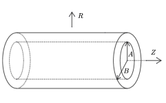
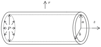
We consider a sufficiently long circular cylindrical tube that is incompressible, isotropic and hyperelastic. The tube is assumed to have inner radius $A$ and outer radius $B$ before deformation; see Fig. 1(a). When it is uniformly stretched in the axial direction by a force $N$ and inflated by an internal pressure $P$, the inner and outer radii become $a$ and $b$, respectively, as shown in Fig. 1(b). The deformation, in terms of cylindrical polar coordinates, is specified by

$\displaystyle r^{2}=\lambda_{z}^{-1}(R^{2}-A^{2})+a^{2},\quad\theta=\Theta,\quad z=\lambda_{z}Z,$

(2.1)

where $(R,\Theta,Z)$ and $(r,\theta,z)$ are the coordinates in the undeformed and deformed configurations, respectively, and $\lambda_{z}$ is the constant stretch in the axial direction. The first equation in (2.1) is a consequence of the incompressibility constraint. It follows from (2.1) that the three principal stretches are simply

$\displaystyle\lambda_{1}=\frac{r}{R},\quad\lambda_{2}=\lambda_{z},\quad\lambda_{3}=1/(\lambda_{1}\lambda_{2}),$

(2.2)

where we have identified the indices $1,2,3$ with the $\theta$-, $z$-, and $r$-directions, respectively. Throughout this paper, we shall refer to the deformed configuration corresponding to (2.1) as the uniformly inflated configuration.

We assume that the constitutive behavior of the tube is described by a strain energy function $W(\lambda_{1},\lambda_{2},\lambda_{3})$. The non-zero Cauchy stresses are given by

$\displaystyle\sigma_{ii}=\lambda_{i}\frac{\partial W}{\partial\lambda_{i}}-\overline{p},\quad i=1,2,3,$

(2.3)

where $\overline{p}$ is the Lagrange multiplier enforcing the incompressibility constraint. For the considered deformation, $W$ can be regarded as a function of $\lambda_{1}$ and $\lambda_{2}$ which we write as $w(\lambda_{1},\lambda_{2})=W(\lambda_{1},\lambda_{2},\lambda_{1}^{-1}\lambda_{2}^{-1})$. By a standard calculation using (2.3) we obtain the stress differences

$\displaystyle\sigma_{11}-\sigma_{33}=\lambda_{1}w_{1},\quad\sigma_{22}-\sigma_{33}=\lambda_{2}w_{2},$

(2.4)

where $w_{1}=\partial w/\partial\lambda_{1}$ and $w_{2}=\partial w/\partial w_{2}$.

The only equilibrium equation that is not satisfied automatically is

$\displaystyle\frac{d\sigma_{33}}{dr}+\frac{\sigma_{33}-\sigma_{11}}{r}=\frac{d\sigma_{33}}{dr}-\frac{\lambda_{1}w_{1}}{r}=0,$

(2.5)

and the associated boundary conditions are

	$\displaystyle\sigma_{33}|_{r=a}=-P,\quad\sigma_{33}|_{r=b}=0,$		(2.6)
	$\displaystyle\int_{a}^{b}r\sigma_{22}\,dr-\frac{1}{2}a^{2}P=\frac{N}{2\pi}.$		(2.7)

Integrating equation (2.5) subject to the boundary conditions (2.6) leads to

$$-\int_{a}^{b}\frac{\lambda w_{1}}{r}\,dr+P=0,$$

(2.8)

whereas eliminating $\sigma_{22}$ in (2.7) in favor of $\sigma_{33}$ with the aid of (2.4)₂, (2.5) and (2.6) yields

$$\int_{a}^{b}r\lambda_{z}w_{2}\,dr-\frac{1}{2}\int_{a}^{b}r\lambda w_{1}\,dr-\frac{N}{2\pi}=0.$$

(2.9)

Alternatively, the last two equations may be manipulated into the form [29]

	$\displaystyle P=\int_{\lambda_{b}}^{\lambda_{a}}\frac{w_{1}}{\lambda^{2}\lambda_{z}-1}\,d\lambda,$		(2.10)
	$\displaystyle N=\pi A^{2}(\lambda_{a}^{2}\lambda_{z}-1)\int_{\lambda_{b}}^{\lambda_{a}}\frac{2\lambda_{z}w_{2}-\lambda w_{1}}{(\lambda^{2}\lambda_{z}-1)^{2}}\lambda\,d\lambda,$		(2.11)

where the two limits $\lambda_{a}$ and $\lambda_{b}$ are defined by $\lambda_{a}=a/A$ and $\lambda_{b}=b/B$, and are related to each other by the incompressibility condition $(\lambda_{b}^{2}\lambda_{z}-1)B^{2}=(\lambda_{a}^{2}\lambda_{z}-1)A^{2}$.

We first summarize the linearized incremental equations for the problem formulated in the previous subsection. We consider an axisymmetric perturbation of the form

$\displaystyle\delta\bm{x}=u(r,z)\bm{e}_{r}+v(r,z)\bm{e}_{z},$

(2.12)

where $\delta\bm{x}$ stands for the increment of the position vector $\bm{x}$ and $(\bm{e}_{r},\bm{e}_{\theta},\bm{e}_{z})$ denotes the standard orthonormal basis for cylindrical polar coordinates $(r,\theta,z)$. It follows that the incremental deformation gradient $\bm{\eta}$ is

$\displaystyle\bm{\eta}=\frac{u}{r}\bm{e}_{\theta}\otimes\bm{e}_{\theta}+v_{z}\bm{e}_{z}\otimes\bm{e}_{z}+v_{r}\bm{e}_{z}\otimes\bm{e}_{r}+u_{z}\bm{e}_{r}\otimes\bm{e}_{z}+u_{r}\bm{e}_{r}\otimes\bm{e}_{r},$

(2.13)

where $v_{z}:=\partial v/\partial z$, $v_{r}:=\partial v/\partial r$, etc.

The incremental equilibrium equations that are not satisfied automatically are [15]

	$\displaystyle\frac{\partial\chi_{22}}{\partial z}+\frac{\partial\chi_{23}}{\partial r}+\frac{\chi_{23}}{r}=0,$		(2.14)
	$\displaystyle\frac{\partial\chi_{33}}{\partial r}+\frac{\partial\chi_{32}}{\partial z}+\frac{\chi_{33}-\chi_{11}}{r}=0,$		(2.15)

where the incremental stress components $\chi_{ij}$ are given by

$\displaystyle\chi_{ij}=\mathcal{B}_{jikl}\eta_{lk}+\overline{p}\eta_{ji}-p^{*}\delta_{ji}.$

(2.16)

In the above expression, $\overline{p}$ and $p^{*}$ are the Lagrange multipliers associated with the deformation (2.1) and the incremental deformation, respectively, and $\mathcal{B}_{ijkl}$ are the instantaneous elastic moduli given by [28]

$\displaystyle\begin{split}&\mathcal{B}_{iijj}=\lambda_{i}\lambda_{j}W_{ij},\\ &\mathcal{B}_{ijij}=\frac{\lambda_{i}W_{i}-\lambda_{j}W_{j}}{\lambda_{i}^{2}-\lambda_{j}^{2}}\lambda_{i}^{2},\quad\lambda_{i}\neq\lambda_{j},\\ &\mathcal{B}_{ijji}=\mathcal{B}_{ijij}-\lambda_{i}W_{i},\quad i\neq j,\end{split}$

(2.17)

where $W_{i}=\partial W/\partial\lambda_{i}$, $W_{ij}=\partial^{2}W/\partial\lambda_{i}\partial\lambda_{j}$, etc.

The equilibrium equations (2.14) and (2.15) are to be solved in conjunction with the incompressibility condition

$\displaystyle\operatorname{tr}(\bm{\eta})=u_{r}+v_{z}+\frac{u}{r}=0$

(2.18)

subject to the incremental boundary conditions

$\displaystyle(\bm{\chi}\bm{n}-P\bm{\eta}^{T}\bm{n})|_{r=a}=0,\quad\bm{\chi}\bm{n}|_{r=b}=0,$

(2.19)

where $\bm{n}$ denotes the unit normal to the surface where each of the boundary conditions is imposed. Written out explicitly, the above boundary conditions become

	$\displaystyle v_{r}+u_{z}=0,\quad r=a,b,$		(2.20)
	$\displaystyle(\mathcal{B}_{3333}-\mathcal{B}_{2233}+\lambda_{3}W_{3})u_{r}+(\mathcal{B}_{1133}-\mathcal{B}_{2233})\frac{u}{r}-p^{*}=0,\quad r=a,b.$		(2.21)

To study the bifurcation of the primary deformation determined previously, we look for an eigensolution of the form

$\displaystyle u(r,z)=f(r)e^{\alpha z},\quad v(r,z)=\frac{1}{\alpha}g(r)e^{\alpha z},\quad p^{*}(r,z)=h(r)e^{\alpha z},$

(2.22)

where $\alpha$ is a spectral parameter and the functions $f,g$ and $h$ are to be determined. On substituting these expressions into (2.14), (2.15) and (2.18)–(2.21), we obtain the differential equations

	$\displaystyle\begin{split}&\alpha^{2}(\mathcal{B}_{2233}+\mathcal{B}_{3223})f^{\prime}(r)+\alpha^{2}\frac{1}{r}(r(\mathcal{B}_{3223}^{\prime}+\overline{p}^{\prime})+\mathcal{B}_{1122}+\mathcal{B}_{3223})f(r)\\ &+\mathcal{B}_{3232}g^{\prime\prime}(r)+\frac{1}{r}(\mathcal{B}_{3232}+r\mathcal{B}_{3232}^{\prime})g^{\prime}(r)+\alpha^{2}\mathcal{B}_{2222}g(r)-\alpha^{2}h(r)=0,\end{split}$			(2.23)
	$\displaystyle\begin{split}&\mathcal{B}_{3333}f^{\prime\prime}(r)+\frac{1}{r}(r(\mathcal{B}^{\prime}_{3333}+\overline{p}^{\prime})+\mathcal{B}_{3333})f^{\prime}(r)+\frac{1}{r^{2}}(\alpha^{2}r^{2}\mathcal{B}_{2323}+r\mathcal{B}_{1133}^{\prime}-\mathcal{B}_{1111})f(r)\\ &+(\mathcal{B}_{2233}+\mathcal{B}_{2332})g^{\prime}(r)+\frac{1}{r}(r\mathcal{B}_{2233}^{\prime}+\mathcal{B}_{2233}-\mathcal{B}_{1122})g(r)-h^{\prime}(r)=0,\end{split}$			(2.24)
		$\displaystyle f^{\prime}(r)+\frac{f(r)}{r}+g(r)=0,$		(2.25)

and the associated boundary conditions

	$\displaystyle\alpha^{2}f(r)+g^{\prime}(r)=0,\quad r=a,b,$		(2.26)
	$\displaystyle(\mathcal{B}_{3333}-\mathcal{B}_{2233}+\lambda_{3}W_{3})f^{\prime}(r)+\frac{1}{r}(\mathcal{B}_{1133}-\mathcal{B}_{2233})f(r)-h(r)=0,\ r=a,b.$		(2.27)

In the above equations, $\mathcal{B}_{3223}^{\prime}=d\mathcal{B}_{3223}/dr$, $\overline{p}^{\prime}=d\overline{p}/dr$, etc. Solving the above eigenvalue problem using the numerical scheme detailed in [14] or [29], we may determine the relationship between $\lambda_{a}$ and $\alpha^{2}$. For periodic buckling modes, we replace $\alpha$ by ${\rm i}k$ with $k$ denoting the axial wavenumber. The bifurcation condition for such periodic buckling modes has been computed by Haughton & Ogden [29]. Here our attention will be focused on the condition when non-trivial solutions with an infinitesimal $\alpha$ may exist.

We thus assume that $\alpha$ is infinitesimal and write $\varepsilon=\alpha^{2}$. We aim to determine the corresponding principal stretch $\lambda_{a}$ for which such a small eigenvalue can exist (the other parameter $\lambda_{z}$ is either fixed or determined by the condition that $N$ is fixed). Since $\varepsilon$ is small, it is natural to look for a solution of the form

$$\lambda_{a}=\lambda_{a\text{cr}}+\varepsilon\lambda_{0}+O(\varepsilon^{2}).$$

(2.28)

Once we have found this asymptotic expression, it is then clear that $\alpha\to 0$ as $\lambda_{a}\to\lambda_{a\text{cr}}$. In other words, $\lambda_{a\text{cr}}$ is the value of $\lambda_{a}$ at which zero becomes a triple eigenvalue and is therefore the critical value for localized bulging to take place [30, 31, 32].

Since the eigenvalue problem (LABEL:eq:g)–(2.27) contains a small parameter ${\varepsilon}$, it is appropriate to look for an asymptotic solution of the form

$\displaystyle\begin{split}&f(r)=\varepsilon f^{(1)}(r)+{\varepsilon}^{2}f^{(2)}(r)+\cdots,\\ &g(r)=\varepsilon g^{(1)}(r)+{\varepsilon}^{2}g^{(2)}(r)+\cdots,\\ &h(r)=\varepsilon h^{(1)}(r)+{\varepsilon}^{2}h^{(2)}(r)+\cdots,\end{split}$

(2.29)

where the functions on the right-hand sides are to be determined at successive orders.

On substituting (2.29) into (LABEL:eq:g), (2.25), (2.26), and then equating the coefficients of $\varepsilon$, we obtain

	$\displaystyle\frac{1}{r}\frac{d}{dr}r\mathcal{B}_{3232}\frac{d}{dr}g^{(1)}=0,\quad g^{(1)}+\frac{1}{r}\frac{d}{dr}rf^{(1)}=0,$		(2.30)
	$\displaystyle\frac{d}{dr}g^{(1)}=0,\quad\ r=a,b.$		(2.31)

By straightforward integration, we find that

$\displaystyle g^{(1)}=-2c_{1},\quad f^{(1)}=c_{1}r+\frac{c_{2}}{r},$

(2.32)

where $c_{1}$ and $c_{2}$ are arbitrary constants.

The solution for $h^{(1)}(r)$ can be found by considering the coefficients of $\varepsilon$ in the equilibrium equation (LABEL:eq:f) and the associated boundary conditions (2.27), which take the form

	$\displaystyle c_{1}\omega_{1}(r)+c_{2}\omega_{2}(r)-\frac{d}{dr}h^{(1)}=0,$		(2.33)
	$\displaystyle c_{1}D_{1}(r)+c_{2}D_{2}(r)-h^{(1)}=0,\quad r=a,b,$		(2.34)

where the functions $\omega_{1}(r)$, $\omega_{2}(r)$, $D_{1}(r)$ and $D_{2}(r)$ are defined by

	$\displaystyle\omega_{1}(r)=\mathcal{B}^{\prime}_{1133}+\mathcal{B}^{\prime}_{3333}-2\mathcal{B}^{\prime}_{2233}+\bar{p}^{\prime}+\frac{1}{r}(2\mathcal{B}_{1122}+\mathcal{B}_{3333}-\mathcal{B}_{1111}-2\mathcal{B}_{2233}),$		(2.35)
	$\displaystyle\omega_{2}(r)=\frac{1}{r^{2}}(\mathcal{B}^{\prime}_{1133}-\mathcal{B}^{\prime}_{3333}-\bar{p}^{\prime})+\frac{1}{r^{3}}(\mathcal{B}_{3333}-\mathcal{B}_{1111}),$		(2.36)
	$\displaystyle D_{1}(r)=\mathcal{B}_{1133}+\mathcal{B}_{3333}-2\mathcal{B}_{2233}+\lambda_{3}W_{3},$		(2.37)
	$\displaystyle D_{2}(r)=\frac{1}{r^{2}}(\mathcal{B}_{1133}-\mathcal{B}_{3333}-\lambda_{3}W_{3}).$		(2.38)

Integrating (2.33) from $r=a$ to $r=b$ and making use of the boundary condition (2.34), we obtain

$\displaystyle m_{11}c_{1}+m_{12}c_{2}=0,$

(2.39)

where the coefficients $m_{11}$ and $m_{12}$ are given by

	$\displaystyle m_{11}=\int_{a}^{b}\omega_{1}(r)\,dr+D_{1}(a)-D_{1}(b),$		(2.40)
	$\displaystyle m_{12}=\int_{a}^{b}\omega_{2}(r)\,dr+D_{2}(a)-D_{2}(b).$		(2.41)

Alternatively, equation (2.39) can be obtained by integrating the equilibrium equation (2.15) from $r=a$ to $r=b$ and making use of the boundary conditions (2.19), that is from

$\displaystyle\int_{a}^{b}\frac{\partial\chi_{32}}{\partial z}\,dr+\int_{a}^{b}\frac{\chi_{33}-\chi_{11}}{r}\,dr-Pu_{r}|_{r=a}=0.$

(2.42)

A second linear equation for $c_{1}$ and $c_{2}$ can be derived from overall equilibrium in the $z$-direction:

$\displaystyle\int_{a}^{b}\chi_{22}r\,dr-Pau|_{r=a}=0.$

(2.43)

This equation follows from integration of the equilibrium equation (2.14) multiplied by $r$ from $r=a$ to $r=b$, followed by application of the boundary conditions (2.19) and the decaying conditions as $z\to\pm\infty$ appropriate for a localized solution. Equating the coefficient of $\varepsilon$ in the above equation then leads to

$\displaystyle m_{21}c_{1}+m_{22}c_{2}=0,$

(2.44)

where the coefficients $m_{21}$ and $m_{22}$ are given by

	$\displaystyle m_{21}=\int_{a}^{b}\theta_{1}(r)r\,dr-\frac{1}{2}\int_{a}^{b}\omega_{1}(r)(b^{2}-r^{2})\,dr-\frac{1}{2}D_{1}(a)(b^{2}-a^{2})-a^{2}P,$		(2.45)
	$\displaystyle m_{22}=\int_{a}^{b}\theta_{2}(r)r\,dr-\frac{1}{2}\int_{a}^{b}\omega_{2}(r)(b^{2}-r^{2})\,dr-\frac{1}{2}D_{2}(a)(b^{2}-a^{2})-P,$		(2.46)

with $\theta_{1}(r)$ and $\theta_{2}(r)$ defined by

	$\displaystyle\theta_{1}(r)=\mathcal{B}_{1122}+\mathcal{B}_{2233}-2\mathcal{B}_{2222}-2\overline{p},$		(2.47)
	$\displaystyle\theta_{2}(r)=\frac{1}{r^{2}}(\mathcal{B}_{1122}-\mathcal{B}_{2233}).$		(2.48)

The existence of a nonzero solution to (2.39) and (2.44) requires that

$\displaystyle\Omega(\lambda_{a},\lambda_{z}):=m_{11}m_{22}-m_{12}m_{21}=0,$

(2.49)

which is an equation that must be satisfied by $\lambda_{a\text{cr}}$, and so is the bifurcation condition for localized bulging. We have verified numerically that (2.49) is equivalent to its counterpart in [14]. We note that equations (2.39) and (2.44) are both obtained at leading order due to the use of two integrals of the incremental equilibrium equations, whereas their counterparts in [14] were obtained at a higher order.

Although the bifurcation condition (2.49) is simpler than its counterpart in [14], it is still too complicated to give a direct analytical proof of its equivalence to $J(P,N)=0$, where $J(P,N)$ denotes the Jacobian of $P$ and $N$ with each of them viewed as a function of $\lambda_{a}$ and $\lambda_{z}$ (see (2.10) and (2.11)). Previously, this equivalence was only shown numerically by verifying that the contour plots of $\Omega(\lambda_{a},\lambda_{z})=0$ and $J(P,N)=0$ in the $(\lambda_{a},\lambda_{z})$-plane always coincide. We now establish this equivalence analytically.

We first note that with the use of (2.29) and (2.32), the solution (2.22) takes the form

	$\displaystyle u(r,z)=\alpha^{2}(c_{1}r+\frac{c_{2}}{r}+O(\alpha^{2}))e^{\alpha z},$		(2.50)
	$\displaystyle v(r,z)=\alpha(-2c_{1}+O(\alpha^{2}))e^{\alpha z}.$		(2.51)

Thus, to order $\alpha^{2}$ we have

$\displaystyle u(r,z)=\alpha^{2}(c_{1}r+\frac{c_{2}}{r}),\quad v(r,z)=-2\alpha c_{1}-2\alpha^{2}c_{1}z.$

(2.52)

Consequently, the coordinates of a representative point in the perturbed configuration are given by

$\displaystyle\tilde{r}=r+\alpha^{2}(c_{1}r+\frac{c_{2}}{r}),\quad\tilde{z}=z-2\alpha^{2}c_{1}z-2\alpha c_{1}.$

(2.53)

To interpret these two expressions, we view the $r$ and $z$ given by (2.1) as functions of $\lambda_{a}$ and $\lambda_{z}$ and differentiate them to obtain

	$\displaystyle dr=\frac{\partial r}{\partial\lambda_{a}}d\lambda_{a}+\frac{\partial r}{\partial\lambda_{z}}d\lambda_{z}=\frac{A^{2}\lambda_{a}}{r}d\lambda_{a}-\frac{r^{2}-A^{2}\lambda_{a}^{2}}{2r\lambda_{z}}d\lambda_{z},$		(2.54)
	$\displaystyle dz=\lambda_{z}^{-1}zd\lambda_{z},$		(2.55)

where $dr$ denotes the differential of $r$ etc. It can then be verified that equation (2.53) may be rewritten as $\tilde{r}=r+dr$, $\tilde{z}=z+dz-2\alpha c_{1}$ provided

$\displaystyle d\lambda_{a}=\alpha^{2}(c_{1}\lambda_{a}+\frac{c_{2}}{\lambda_{a}A^{2}}),\quad d\lambda_{z}=-2\alpha^{2}\lambda_{z}c_{1}.$

(2.56)

Thus, the perturbed configuration given by (2.53) is due to a constant perturbation in $\lambda_{a}$ and $\lambda_{z}$. In other words, the solution (2.52) corresponds to a perturbation that takes the hyperelastic tube from one uniformly inflated configuration to another uniformly inflated configuration, plus a rigid body displacement in the axial direction (represented by the term $-2\alpha c_{1}$). Note that higher order terms are not relevant to the bifurcation condition since as pointed earlier the latter was derived at leading order. Therefore, the bifurcation condition for localized bulging is simply the condition for an adjacent uniformly inflated configuration to exist.

Let us denote by $P^{*}(\lambda_{a},\lambda_{z})$ and $N^{*}(\lambda_{a},\lambda_{z})$ the two functions resulting from viewing $P$ and $N$ as functions of $\lambda_{a}$ and $\lambda_{z}$ (i.e., the right-hand sides of (2.10) and (2.11)). Then uniformly inflated configurations are characterized by the following two equations

$\displaystyle P^{*}(\lambda_{a},\lambda_{z})=P,\quad N^{*}(\lambda_{a},\lambda_{z})=N.$

(2.57)

As argued above, the bifurcation occurs when locally the above relation cannot be inverted uniquely. By the implicit function theorem, this implies that the Jacobian determinant of the functions $P^{*}$ and $N^{*}$ is zero at the bifurcation point. We note that $P^{*}(\lambda_{a},\lambda_{z})$ and $N^{*}(\lambda_{a},\lambda_{z})$ represent the functional dependence of $P$ and $N$ on $\lambda_{a}$ and $\lambda_{z}$, respectively. Hence the bifurcation condition for localized bulging is equivalent to the vanishing of the Jacobian of $P$ and $N$ with them viewed as functions of $\lambda_{a}$ and $\lambda_{z}$.

By carefully analyzing the linearized forms of (2.57) and connecting them with equations (2.42) and (2.43), one can establish the equality

$\displaystyle\Omega(\lambda_{a},\lambda_{z})=-\frac{\lambda_{z}}{\pi\lambda_{a}A^{2}}\Big{(}\frac{\partial P^{*}}{\partial\lambda_{a}}\frac{\partial N^{*}}{\partial\lambda_{z}}-\frac{\partial P^{*}}{\partial\lambda_{z}}\frac{\partial N^{*}}{\partial\lambda_{a}}\Big{)},$

(2.58)

which proves the equivalence between the bifurcation condition and $J(P,N)=0$ explicitly in view of (2.49). For interested readers, we present the proof of equality (2.58) in Appendix A.

We consider a sufficiently large circular incompressible hyperelastic sheet that is subject to an equibiaxial tension in its plane. The thicknesses of the sheet in the undeformed and deformed configurations are denoted by $2H$ and $2h$, respectively. The equibiaxial deformation is described by

$\displaystyle r=\lambda R,\quad\theta=\Theta,\quad z=\lambda^{-2}Z,$

(3.1)

where $(R,\Theta,Z)$ and $(r,\theta,z)$ are the cylindrical polar coordinates in the undeformed and deformed configurations, respectively, and $\lambda$ is the constant stretch in the plane. It follows that the three principal stretches are given by

$\displaystyle\lambda_{1}=\lambda_{3}=\lambda,\quad\lambda_{2}=\lambda^{-2},$

(3.2)

where $1$, $2$, $3$ still correspond to the $\theta$-, $z$- and $r$-directions, respectively.

In terms of the strain energy function $W(\lambda_{1},\lambda_{2},\lambda_{3})$, the non-zero nominal stress components are given by

$\displaystyle S_{ii}=\frac{\partial W}{\partial\lambda_{i}}-\overline{p}\lambda_{i}^{-1},\quad i=1,2,3,$

(3.3)

where $\overline{p}$ is the Lagrange multiplier enforcing the incompressibility constraint. The top and bottom surfaces of the sheet are assumed to be traction-free, thus $S_{22}=0$. Eliminating $\overline{p}$ using this condition yields

$\displaystyle S_{11}(\lambda_{1},\lambda_{3})=\frac{\partial w}{\partial\lambda_{1}}(\lambda_{1},\lambda_{3}),\quad S_{33}(\lambda_{1},\lambda_{3})=\frac{\partial w}{\partial\lambda_{3}}(\lambda_{1},\lambda_{3}),$

(3.4)

where $w(\lambda_{1},\lambda_{3})=W(\lambda_{1},\lambda_{1}^{-1}\lambda_{3}^{-1},\lambda_{3})$ is the reduced strain energy function. For the homogeneous solution, we have $2S_{33}=dw(\lambda,\lambda)/d\lambda$, which allows one to determine the stretch once the traction at the circular edge is specified.

In a similar fashion to Section 2, the bifurcation condition for axisymmetric necking can be obtained by solving an eigenvalue problem. As in that section, we superpose an axisymmetric perturbation of the form $\delta\bm{x}=u(r,z)\bm{e}_{r}+v(r,z)\bm{e}_{z}$ to the homogeneous configuration. The linearized incremental governing equations can be written as

	$\displaystyle\frac{\partial\chi_{22}}{\partial z}+\frac{\partial\chi_{23}}{\partial r}+\frac{\chi_{23}}{r}=0,$		(3.5)
	$\displaystyle\frac{\partial\chi_{33}}{\partial r}+\frac{\partial\chi_{32}}{\partial z}+\frac{\chi_{33}-\chi_{11}}{r}=0,$		(3.6)
	$\displaystyle\eta_{11}+\eta_{22}+\eta_{33}=0,$		(3.7)
	$\displaystyle\chi_{22}=0,\quad\chi_{32}=0,\quad z=\pm h,$		(3.8)

where the incremental deformation gradient $\bm{\eta}$ and stress tensor $\bm{\chi}$ have been defined in (2.13) and (2.16), respectively.

We look for an eigensolution of the form

$\displaystyle u(r,z)=\frac{1}{\alpha}f(z)I_{1}(\alpha r),\quad v(r,z)=g(z)I_{0}(\alpha r),\quad p^{*}(r,z)=p(z)I_{0}(\alpha r),$

(3.9)

where $\alpha$ plays the role of the spectral parameter, $I_{n}(x)$, $n=0,1,\dots$ denote the modified Bessel functions of the first kind that obey the identities

$\displaystyle I_{n+1}(x)=I_{n-1}(x)-\frac{2n}{x}I_{n}(x),\quad I^{\prime}_{n}(x)=\frac{1}{2}(I_{n-1}(x)+I_{n+1}(x)),$

(3.10)

and the functions $f$, $g$ and $p$ are to be determined. On substituting this solution into (3.5)–(3.8) and using (3.10) to simplify the results, we obtain the differential equations

	$\displaystyle(\mathcal{B}_{1122}+\mathcal{B}_{3223})f^{\prime}(z)+\mathcal{B}_{2222}g^{\prime\prime}(z)+\alpha^{2}\mathcal{B}_{3232}g(z)-p^{\prime}(z)=0,$		(3.11)
	$\displaystyle\mathcal{B}_{2323}f^{\prime\prime}(z)+\alpha^{2}\mathcal{B}_{1111}f(z)+\alpha^{2}(\mathcal{B}_{1122}+\mathcal{B}_{2332})g^{\prime}(z)-\alpha^{2}p(z)=0,$		(3.12)
	$\displaystyle f(z)+g^{\prime}(z)=0,$		(3.13)

and the associated boundary conditions

	$\displaystyle\mathcal{B}_{1122}f(z)+(\mathcal{B}_{2222}+\lambda_{2}W_{2})g^{\prime}(z)-p(z)=0,\quad z=\pm h,$		(3.14)
	$\displaystyle f^{\prime}(z)+\alpha^{2}g(z)=0,\quad z=\pm h.$		(3.15)

We assume that the bifurcation condition for axisymmetric necking still corresponds to when a non-trivial solution with an infinitesimal $\alpha$ exist. To find this condition, we let $\varepsilon=\alpha^{2}$ and look for an asymptotic solution of the form

$\displaystyle\begin{split}&f(z)=\varepsilon f^{(1)}(z)+{\varepsilon}^{2}f^{(2)}(z)+\cdots,\\ &g(z)=\varepsilon g^{(1)}(z)+{\varepsilon}^{2}g^{(2)}(z)+\cdots,\\ &p(z)=\varepsilon p^{(1)}(z)+{\varepsilon}^{2}p^{(2)}(z)+\cdots.\end{split}$

(3.16)

On substituting (3.16) into (3.11)–$\eqref{eq:add5}$ and equating the coefficient of $\varepsilon$, we obtain a boundary value problem satisfied by $f^{(1)}$, $g^{(1)}$ and $p^{(1)}$ whose solution is given by

$\displaystyle f^{(1)}=A,\quad g^{(1)}=-Az+B,\quad p^{(1)}=A(\mathcal{B}_{1122}-\mathcal{B}_{2222}-\lambda_{2}W_{2}),$

(3.17)

where $A$ and $B$ are arbitrary constants.

By integrating $r$ times the equilibrium equation (3.6) across the thickness and making use of the boundary conditions (3.8), we obtain

$\displaystyle r\frac{d\tilde{\chi}_{33}}{dr}+\tilde{\chi}_{33}-\tilde{\chi}_{11}=0,$

(3.18)

where the stress resultants $\tilde{\chi}_{11}$ and $\tilde{\chi}_{33}$ are defined by

$\displaystyle\tilde{\chi}_{11}=\int_{-h}^{h}\chi_{11}\,dz,\quad\tilde{\chi}_{33}=\int_{-h}^{h}\chi_{33}\,dz.$

(3.19)

Substituting (3.17) into (3.18), we obtain

$\displaystyle\begin{split}r\frac{d\tilde{\chi}_{33}}{dr}+\tilde{\chi}_{33}-\tilde{\chi}_{11}&=(\varepsilon(\mathcal{B}_{1111}+\mathcal{B}_{2222}-2\mathcal{B}_{1122}+2\lambda_{2}W_{2})A+O(\varepsilon^{2}))2h\alpha rI_{1}(\alpha r)\\ &=\varepsilon^{2}(\mathcal{B}_{1111}+\mathcal{B}_{2222}-2\mathcal{B}_{1122}+2\lambda_{2}W_{2})hr^{2}A+O(\varepsilon^{3})=0,\end{split}$

(3.20)

which must hold for arbitrary $\varepsilon$. It follows that the bifurcation condition for axisymmetric necking is [27]

$\displaystyle\mathcal{B}_{1111}+\mathcal{B}_{2222}-2\mathcal{B}_{1122}+2\lambda_{2}W_{2}=0.$

(3.21)

We remark that the leading order term on the right-hand side of (3.20) is of order $\varepsilon^{2}$ and the bifurcation condition is obtained by setting this $\varepsilon^{2}$ term to zero. This is in contrast with the situation in the previous problem where the bifurcation equation was obtained by equating an $O(\varepsilon)$ term to zero.

In view of (3.13) and (3.17), the perturbation solution is of the form

		$\displaystyle u(r,z)=\alpha(A+\alpha^{2}C^{\prime}(z)+O(\alpha^{4}))I_{1}(\alpha r),$		(3.22)
		$\displaystyle v(r,z)=\alpha^{2}(-Az+B-\alpha^{2}C(z)+O(\alpha^{4}))I_{0}(\alpha r),$		(3.23)

where $C(z)=-g^{(2)}(z)$. Note that we cannot obtain the bifurcation condition by expanding $I_{0}(\alpha r)$ and $I_{1}(\alpha r)$ in terms of $\alpha$ and then considering the leading order (i.e., $O(\alpha^{2})$) terms of $u(r,z)$ and $v(r,z)$ as in Subsection 2.3, since now the bifurcation condition is obtained at $O(\alpha^{4})$. To order $\alpha^{4}$, we have

	$\displaystyle u=\frac{1}{2}\alpha^{2}Ar+\frac{1}{16}\alpha^{4}Ar^{3}+\frac{1}{2}\alpha^{4}rC^{\prime}(z),$		(3.24)
	$\displaystyle v=\alpha^{2}(-Az+B)+\frac{1}{4}\alpha^{4}(-Az+B)r^{2}-\alpha^{4}C(z).$		(3.25)

Accordingly, the non-zero components of the incremental deformation gradient to order $\alpha^{4}$ are

$\displaystyle\begin{split}&\eta_{11}=\frac{1}{2}\alpha^{2}A+\frac{1}{16}\alpha^{4}Ar^{2}+\frac{1}{2}\alpha^{4}C^{\prime}(z),\\ &\eta_{22}=-\alpha^{2}A-\frac{1}{4}\alpha^{4}Ar^{2}-\alpha^{4}C^{\prime}(z),\\ &\eta_{23}=\frac{1}{2}\alpha^{4}(-Az+B)r,\\ &\eta_{32}=\frac{1}{2}\alpha^{4}rC^{\prime\prime}(z),\\ &\eta_{33}=\frac{1}{2}\alpha^{2}A+\frac{3}{16}\alpha^{4}Ar^{2}+\frac{1}{2}\alpha^{4}C^{\prime}(z).\end{split}$

(3.26)

Let $\bm{F}$ denote the deformation gradient related to the perturbed deformation. It follows from the chain rule that

$\displaystyle\bm{F}=\begin{pmatrix}\lambda(1+\eta_{11})&0&0\\ 0&\lambda^{-2}(1+\eta_{22})&\lambda\eta_{23}\\ 0&\lambda^{-2}\eta_{32}&\lambda(1+\eta_{33})\end{pmatrix}.$

(3.27)

The corresponding principal stretches are then given by

$\displaystyle\tilde{\lambda}_{1}=\lambda(1+\eta_{11}),\quad\tilde{\lambda}_{2}=\lambda^{-2}(1+\eta_{22})+O(\alpha^{8}),\quad\tilde{\lambda}_{3}=\lambda(1+\eta_{33})+O(\alpha^{8}).$

(3.28)

Thus even to order $\alpha^{4}$, the $\theta$-, $z$- and $r$-directions are still principal directions, and the constitutive relation (3.4) still holds for the perturbed configuration. We note, however, that the deformation is homogeneous (an equibiaxial extension) to order $\alpha^{2}$, but is non-homogeneous when expanded to order $\alpha^{4}$.

References

- [1] Mallock, A.: Note on the instability of India-rubber tubes and balloons when distended by fluid pressure. Proc. Roy. Soc. A 49, 458–463 (1891). https://doi.org/10.1098/rspl.1890.0116
- [2] Yin, W.-L.: Non-uniform inflation of a cylindrical elastic membrane and direct determination of the strain energy function. J. Elast. 7, 265–282 (1977). https://doi.org/10.1007/BF00041073
- [3] Chater, E., Hutchinson, J.W.: On the propagation of bulges and buckles. J. Appl. Mech. 51, 269–277 (1984). https://doi.org/10.1115/1.3167611
- [4] Kyriakides, S., Chang, Y.-C.: On the inflation of a long elastic tube in the presence of axial load. Int. J. Solids Struct. 26(9–10), 975–991 (1990). https://doi.org/10.1016/0020-7683(90)90012-K
- [5] Kyriakides, S., Chang, Y.-C.: The initiation and propagation of a localized instability in an inflated elastic tube. Int. J. Solids Struct. 27(9), 1085–1111 (1991). https://doi.org/10.1016/0020-7683(91)90113-T
- [6] Pamplona, D. C., Goncalves, P. B., Lopes, S. R. X.: Finite deformations of cylindrical membrane under internal pressure. Int. J. Mech. Sci. 48(6), 683–696 (2006). https://doi.org/10.1016/j.ijmecsci.2005.12.007
- [7] Goncalves, P. B., Pamplona, D., Lopes, S. R. X.: Finite deformations of an initially stressed cylindrical shell under internal pressure. Int. J. Mech. Sci. 50(1), 92–103 (2008). https://doi.org/10.1016/j.ijmecsci.2007.05.001
- [8] Rodríguez, J., Merodio, J.: A new derivation of the bifurcation conditions of inflated cylindrical membranes of elastic material under axial loading. Application to aneurysm formation. Mech. Re. Commun. 38(3), 203–210, (2011). https://doi.org/10.1016/j.mechrescom.2011.02.004
- [9] Alhayani, A.A., Rodríguez, J., Merodio, J.: Competition between radial expansion and axial propagation in bulging of inflated cylinders with application to aneurysms propagation in arterial wall tissue. Int. J. Eng. Sci. 85, 74–89 (2014). https://doi.org/10.1016/j.ijengsci.2014.08.008
- [10] Alexander, H.: Tensile instability of initially spherical balloons. Int. J. Eng. Sci. 9, 151–160 (1971). https://doi.org/10.1016/0020-7225(71)90017-6
- [11] Kanner, L. M., Horgan, C.O.: Elastic instabilities for strain-stiffening rubber-like spherical and cylindrical thin shells under inflation. Int. J. Non-linear Mech. 42, 204–215 (2007). https://doi.org/10.1016/j.ijnonlinmec.2006.10.010
- [12] Horny, L., Netusil, M., Horak, Z.: Limit point instability in pressurization of anisotropic finitely extensible hyperelastic thin-walled tube. Int. J. Non-linear Mech. 77, 107–114 (2015). https://doi.org/10.1016/j.ijnonlinmec.2015.08.003
- [13] Fu, Y.B., Pearce, S.P., Liu, K.K.: Post-bifurcation analysis of a thin-walled hyperelastic tube under inflation. Int. J. Non-linear Mech. 43(8), 697–706 (2008). https://doi.org/10.1016/j.ijnonlinmec.2008.03.003
- [14] Fu, Y.B., Liu, J.L., Francisco, G.S.: Localized bulging in an inflated cylindrical tube of arbitrary thickness–the effect of bending stiffness. J. Mech. Phys. Solids, 90, 45–60 (2016). https://doi.org/10.1016/j.jmps.2016.02.027
- [15] Ye, Y., Liu, Y., Fu, Y.B.: Weakly nonlinear analysis of localized bulging of an inflated hyperelastic tube of arbitrary wall thickness. J. Mech. Phys. Solids 135, 103804 (2020). https://doi.org/10.1016/j.jmps.2019.103804
- [16] Lin, Z., Li, L., Ye, Y.: Numerical simulation of localized bulging in an inflated hyperelastic tube with fixed ends. Int. J. Appl. Mech. 12(10), 2050118 (2020). https://doi.org/10.1142/S1758825120501185
- [17] Wang, S., Guo, Z., Zhou, L., Li, L., Fu, Y.B.: An experimental study of localized bulging in inflated cylindrical tubes guided by newly emerged analytical results. J. Mech. Phys. Solids 124, 536–554 (2019). https://doi.org/10.1016/j.jmps.2018.11.011
- [18] Varatharajan, N., DasGupta, A.: Study of bifurcation in a pressurized hyperelastic membrane tube enclosed by a soft substrate. Int. J. Non-linear Mech. 95, 233–241 (2017). https://doi.org/10.1016/j.ijnonlinmec.2017.05.004
- [19] Wang, J., Althobaiti, A., Fu, Y. B.: Localized bulging of rotating elastic cylinders and tubes. J. Mech. Mater. Struct. 12(4), 545–561 (2017). http://dx.doi.org/10.2140/jomms.2017.12.545
- [20] Wang, J., Fu, Y.B. (2018).: Effect of double-fibre reinforcement on localized bulging of an inflated cylindrical tube of arbitrary thickness. J. Eng. Math. 109(1), 21–30. https://doi.org/10.1007/s10665-017-9899-5
- [21] Liu, Y., Ye, Y., Althobaiti, A., Xie, Y. X.: Prevention of localized bulging in an inflated bilayer tube. Int. J. Mech. Sci. 153, 359–368 (2019). https://doi.org/10.1016/j.ijmecsci.2019.01.028
- [22] Ye, Y., Liu, Y., Althobaiti, A., Xie, Y. X.: Localized bulging in an inflated bilayer tube of arbitrary thickness: Effects of the stiffness ratio and constitutive model. Int. J. Solids Struct. 176, 173–184 (2019). https://doi.org/10.1016/j.ijsolstr.2019.06.009
- [23] Hejazi, M., Hsiang, Y., Srikantha Phani, A.: Fate of a bulge in an inflated hyperelastic tube: theory and experiment. Proc. Roy. Soc. A 477(2247), 20200837 (2021). https://doi.org/10.1098/rspa.2020.0837
- [24] Fu, Y.B., Jin, L., Goriely, A.: Necking, beading, and bulging in soft elastic cylinders. J. Mech. Phys. Solids 147, 104250 (2021). https://doi.org/10.1016/j.jmps.2020.104250
- [25] Emery, D., Fu, Y.B.: localized bifurcation in soft cylindrical tubes under axial stretching and surface tension. Int. J. Solids Struct. 219, 23–33 (2021). https://doi.org/10.1016/j.ijsolstr.2021.02.007
- [26] Emery, D., Fu, Y.B.: Post-bifurcation behaviour of elasto-capillary necking and bulging in soft tubes. Proc. R. Soc. A 477, 20210311 (2021). https://doi.org/10.1098/rspa.2021.0311
- [27] Wang, M., Jin, L.S., Fu, Y.B.: Axi-symmetric necking versus Treloar-Kearsley instability in a hyperelastic sheet under equibiaxial stretching. Math. Mech. Solids, February 2022. doi:10.1177/10812865211072897. https://doi.org/10.1177/10812865211072897
- [28] Ogden, R.W.: Non-linear elastic deformations. Ellis Horwood, New York (1984).
- [29] Haughton, D.M., Ogden, R.W.: Bifurcation of inflated circular cylinders of elastic material under axial loading - I. Exact theory for thick-walled tubes. J. Mech. Phys. Solids 27(5-6), 489–512 (1979). https://doi.org/10.1016/0022-5096(79)90001-2
- [30] Kirchgässner, K.: Wave-solutions of reversible systems and applications. J. Diff. Eq., 45(1), 113–127 (1982). https://doi.org/10.1016/0022-0396(82)90058-4
- [31] Mielke, A.: Hamiltonian and Lagrangian flows on center manifolds, with applications to elliptic variational problems. Springer-Verlag, Berlin Lecture Notes in Mathematics (1991).
- [32] Haragus, M., Iooss, G.: Local bifurcations, center manifolds, and normal forms in infinite-dimensional dynamical systems. Springer, London (2011).
- [33] Wang, M., Fu, Y.B.: Necking of a hyperelastic solid cylinder under axial stretching: Evaluation of the infinite-length approximation. Int. J. Eng. Sci., 159, 103432 (2021). https://doi.org/10.1016/j.ijengsci.2020.103432