An adaptive wavelet method for nonlinear partial differential equations with applications to dynamic damage modeling

Cale Harnish Luke Dalessandro Karel Matouš [email protected] Daniel Livescu Department of Aerospace and Mechanical Engineering, University of Notre Dame, Notre Dame, Indiana 46556, USA Department of Intelligent Systems Engineering, Indiana University, Bloomington, Indiana 47405, USA Computer and Computational Sciences Division, Los Alamos National Laboratory, Los Alamos, New Mexico 87545, USA

Abstract

Multiscale and multiphysics problems need novel numerical methods in order for them to be solved correctly and predictively. To that end, we develop a wavelet based technique to solve a coupled system of nonlinear partial differential equations (PDEs) while resolving features on a wide range of spatial and temporal scales. The algorithm exploits the multiresolution nature of wavelet basis functions to solve initial-boundary value problems on finite domains with a sparse multiresolution spatial discretization. By leveraging wavelet theory and embedding a predictor-corrector procedure within the time advancement loop, we dynamically adapt the computational grid and maintain accuracy of the solutions of the PDEs as they evolve. Consequently, our method provides high fidelity simulations with significant data compression. We present verification of the algorithm and demonstrate its capabilities by modeling high-strain rate damage nucleation and propagation in nonlinear solids using a novel Eulerian-Lagrangian continuum framework.

keywords:

Multiresolution analysis, Wavelets, Adaptive algorithm with error control, High-strain rate damage mechanics, High-performance computing

1 Introduction

This work details a novel numerical method capable of modeling multiphysics problems while resolving features on a wide range of spatial and temporal scales. Considering that many engineering applications must incorporate failure modes into material models, the potential of our algorithm is demonstrated by modeling the dynamic damage of a nonlinear solid. The behavior of damaged material has been the subject of extensive research [1, 2, 3, 4, 5, 6, 7, 8, 9, 10, 11, 12, 13, 14, 15]. Early damage models were simple in nature and classified material failure based on comparing the state of stress or strain to empirically measured values [16, 17, 18, 19, 20, 21, 22]. Fracture mechanics provides a more theoretical approach and analytically describes the forces required to open and grow a crack [23, 24, 25]. Alternatively, this work applies thermodynamically consistent computational damage mechanics to model the effects of damage [26].

Continuum damage mechanics has been used to model several failure modes such as: fatigue [27], creep [28], ductile damage [29, 30, 31], brittle damage [32, 33, 34], isotropic damage [35], and anisotropic damage [36, 37]. This work leverages concepts from the reference map technique [38] to extend the Lagrangian constitutive theory from [39, 40, 41] into the Eulerian frame and model rate-dependent isotropic damage. Our coupling of the Eulerian-Lagrangian frames combines the advantages of resolving large deformations on an Eulerian discretization with a constitutive damage model from a Lagrangian description and is one of the novelties of this work. The derivation of the energy based damage model is thermodynamically motivated and incorporates the irreversible nature of the damage process [42, 43].

In general, material failure does not occur only between two adjacent atomic layers [10]. Instead, cracks develop with a finite thickness of a characteristic length-scale, $l_{\omega}$ , and have a process zone at the crack-tip [44, 45, 46, 47]. At the microscale one may find voids and material defects, microcracks can be observed at the mesoscale, and at the macroscale these imperfections coalesce into macrocracks [48]. These features have very small spatial and temporal scales which prove challenging for both experimental measurement [49, 50, 51, 52, 53, 54, 55] and computational modeling [39, 56]. However, computational models of damage have become increasingly important to bridge the gap between theoretical predictions and experimental design.

The computational difficulty of damage modeling has so far been addressed through a variety of numerical techniques. For example, the integral equations from peridynamics are used in [57] to better model the discontinuous nature of cracks. A mesh-free smooth particle hydrodynamic (SPH) simulation was used in [58] to model damage under compressive loading. Finite element methods (FEM) have incorporated rate dependent damage models [59] and cohesive zone models [60] to simulate fracture in brittle materials (e.g., concrete, ceramics, PMMA). The extended finite element method (XFEM) has been used [61] to model a crack with arbitrary discontinuities instead of remeshing. Alternatively, [62, 63] only resolves the damaged material on the microscale and assumes a separation of scales to model its effect on the macroscale using computational homogenization [39, 64, 40, 41]. In contrast, an adaptive space-time discontinuous Galerkin method is used in [65] to provide high resolution simulations, revealing new solution features (e.g., a quasi-singular structure in the velocity response).

In other works, the challenge of multiscale modeling has been met through adaptive mesh refinement (AMR) [66, 67], multigrid methods [68, 69, 70], Chimera overset grids [71], or remeshing/refining FEM [72, 73, 74, 75]. However, these approaches are computationally expensive in the context of damage modeling since the spatial and temporal location of interesting solution features are not known a priori. This work develops an alternative adaptive discretization strategy to resolve all relevant scales from the characteristic length scale of damage to the size of the macroscopic material. In particular, we use wavelet basis functions to approximate solutions to coupled systems of nonlinear partial differential equations (PDEs) in a monolithic multiscale solver.

Wavelet based numerical methods are particularly well suited for modeling multiscale and multiphysics problems, because they can dynamically adapt the discretization to discover spatial scales [76, 77]. Furthermore, current wavelet solvers have achieved several notable accomplishments, including: significant data compression [78, 79, 80], bounded energy conservation [81, 82], modeling stochastic systems [83], multiscale model reduction [84], and solving coupled systems of nonlinear PDEs [85, 86, 87, 88, 89]. However, some implementations only solve PDEs in infinite or periodic domains (e.g., [90, 91, 92]), some do not utilize the data compression ability of wavelets, resulting in a costly uniform grid (e.g., [82, 93, 94]), and some use finite difference methods to calculate the spatial derivatives, reducing the ability to control accuracy (e.g., [85, 86, 87, 95]).

We present a predictor-corrector algorithm designed to advance the state of wavelet-based methods by leveraging the successes of past solvers and developing strategies to mitigate their limitations. We use differentiable wavelet bases to numerically solve nonlinear initial–boundary value problems. We use second-generation wavelets near spatial boundaries to produce multiresolution spatial discretizations on finite domains. Furthermore, the lowest resolution is defined with the minimum number of collocation points required to support the basis functions, thereby improving the ability to compress data. Additionally, we compute spatial derivatives by operating directly on the wavelet bases. We use error estimates for the wavelet representation of fields, their spatial derivatives, and the aliasing errors associated with nonlinear terms to construct a sparse, dynamically adaptive computational grid for each unknown that provides the required accuracy and approaches the theoretical a priori guarantee. Moreover, we employ an embedded Runge-Kutta integration to control the temporal accuracy as the solution of the PDE evolves. Therefore our adaptive multiresolution discretization is guided directly by the wavelet operators and is one of the novelties of this work.

An overview of wavelet theory and the wavelet operations required to solve PDEs is presented in Section 2. Then, our algorithm, the Multiresolution Wavelet Toolkit (MRWT) is described and verification examples are presented in Section 3. Next, the Eulerian-Lagrangian model of dynamic damage growth in nonlinear materials is derived in Section 4. Finally, Section 5 shows results from modeling high-strain rate damage nucleation and propagation, illustrating the benefits of applying this novel numerical method to multiscale and multiphysics problems.

2 Multiresolution analysis

The proposed numerical method exploits the properties of wavelet basis functions and builds the computational grid using the wavelet operators. Therefore it is essential to provide a brief summary of wavelet theory. In particular, the following outlines the construction of wavelet basis functions and defines the operations needed to build a sparse grid and solve nonlinear PDEs.

2.1 Wavelet basis functions

A multiresolution analysis (MRA) provides the formal mathematical definition of a wavelet family of basis functions [96]. An MRA of an $N$ -dimensional domain $\Omega\subset\mathbb{R}^{N}$ consists of a sequence of nested approximation spaces $\boldsymbol{V}_{j}$ and their associated dual spaces $\widetilde{\boldsymbol{V}}_{j}$ such that the union of these spaces is the $L^{2}(\Omega)$ space [97]. The wavelet spaces $\boldsymbol{W}_{j}$ , and their associated dual spaces $\widetilde{\boldsymbol{W}}_{j}$ are then defined as the complements of the approximation spaces $\boldsymbol{V}_{j}$ in $\boldsymbol{V}_{j+1}$ [98, 82]

\displaystyle\boldsymbol{V}_{j}

\displaystyle\subset\boldsymbol{V}_{j+1},

\displaystyle\overline{\bigcup_{j=1}^{\infty}\boldsymbol{V}_{j}}

\displaystyle=L^{2}(\Omega),

\displaystyle\boldsymbol{V}_{j+1}

\displaystyle=\boldsymbol{V}_{j}\oplus\boldsymbol{W}_{j}.

(1)

Furthermore, $N$ -dimensional representations can be constructed through $N$ tensor products of the one-dimensional ( $1$ D) spaces $V_{j}$ and $W_{j}$ . For example, the approximation spaces in a three-dimensional ( $3$ D) setting become

	$\displaystyle\boldsymbol{V}_{j}$	$\displaystyle=V_{j}\otimes V_{j}\otimes V_{j},$
	$\displaystyle\boldsymbol{V}_{j}$	$\displaystyle=\left(V_{j-1}\oplus W_{j-1}\right)\otimes\left(V_{j-1}\oplus W_{j-1}\right)\otimes\left(V_{j-1}\oplus W_{j-1}\right).$		(2)

In general, this produces $2^{N}$ types of basis from each possible combination of $V_{j}$ and $W_{j}$ spaces. The scaling functions $\phi_{k}^{j}(x)$ and dual scaling functions $\widetilde{\phi}_{k}^{j}(x)$ are the $1$ D basis functions in the spaces $V_{j}$ and $\widetilde{V}_{j}$ respectively, whereas the wavelets $\psi_{k}^{j}(x)$ and dual wavelets $\widetilde{\psi}_{k}^{j}(x)$ are the $1$ D basis functions in the spaces $W_{j}$ and $\widetilde{W}_{j}$ respectively. Note that the multiresolution nature of $1$ D wavelets requires the use of two types of indices. One to define the resolution level $j\in\mathbb{Z}$ , and another to define the spatial locations $k\in\mathbb{Z}$ on a particular resolution level $j$ . Furthermore, any basis with $j$ and $k$ designation is constructed through dilations and translations such that

	$\displaystyle\phi_{2k}^{j+1}(x)$	$\displaystyle=\phi_{k}^{j}(2x-2k\Delta x_{j+1}),$	$\displaystyle\widetilde{\phi}_{2k}^{j+1}(x)$	$\displaystyle=2\ \widetilde{\phi}_{k}^{j}(2x-2k\Delta x_{j+1}),$
	$\displaystyle\psi_{2k}^{j+1}(x)$	$\displaystyle=\psi_{k}^{j}(2x-2k\Delta x_{j+1}),$	$\displaystyle\widetilde{\psi}_{2k}^{j+1}(x)$	$\displaystyle=2\ \widetilde{\psi}_{k}^{j}(2x-2k\Delta x_{j+1}),$		(3)

where $\Delta x_{j+1}$ is the grid spacing on level $j+1$ . An additional index $\lambda\in\mathbb{Z}$ is introduced for multidimensional wavelets to simplify notation and denote specific $V_{j}$ and $W_{j}$ combinations as shown in Table 1. The local index $k$ is reset for each $j$ and $\lambda$ combination.

Table 1: Notation for multidimensional basis in

\mathbb{R}^{3}

${}^{\lambda}\Psi_{\vec{k}}^{j}(\vec{x})$	Three-dimensional basis
${}^{0}\Psi_{\vec{k}}^{j}(\vec{x})$	$\phi_{k_{1}}^{j}(x_{1})\ \phi_{k_{2}}^{j}(x_{2})\ \phi_{k_{3}}^{j}(x_{3})$
${}^{1}\Psi_{\vec{k}}^{j}(\vec{x})$	$\psi_{k_{1}}^{j}(x_{1})\ \phi_{k_{2}}^{j}(x_{2})\ \phi_{k_{3}}^{j}(x_{3})$
${}^{2}\Psi_{\vec{k}}^{j}(\vec{x})$	$\phi_{k_{1}}^{j}(x_{1})\ \psi_{k_{2}}^{j}(x_{2})\ \phi_{k_{3}}^{j}(x_{3})$
${}^{3}\Psi_{\vec{k}}^{j}(\vec{x})$	$\psi_{k_{1}}^{j}(x_{1})\ \psi_{k_{2}}^{j}(x_{2})\ \phi_{k_{3}}^{j}(x_{3})$
${}^{4}\Psi_{\vec{k}}^{j}(\vec{x})$	$\phi_{k_{1}}^{j}(x_{1})\ \phi_{k_{2}}^{j}(x_{2})\ \psi_{k_{3}}^{j}(x_{3})$
${}^{5}\Psi_{\vec{k}}^{j}(\vec{x})$	$\psi_{k_{1}}^{j}(x_{1})\ \phi_{k_{2}}^{j}(x_{2})\ \psi_{k_{3}}^{j}(x_{3})$
${}^{6}\Psi_{\vec{k}}^{j}(\vec{x})$	$\phi_{k_{1}}^{j}(x_{1})\ \psi_{k_{2}}^{j}(x_{2})\ \psi_{k_{3}}^{j}(x_{3})$
${}^{7}\Psi_{\vec{k}}^{j}(\vec{x})$	$\psi_{k_{1}}^{j}(x_{1})\ \psi_{k_{2}}^{j}(x_{2})\ \psi_{k_{3}}^{j}(x_{3})$

In many cases the wavelet basis functions do not have a closed-form expression, instead they are defined in terms of four types of filter coefficients (i.e., $h_{i},\ \widetilde{h}_{i},\ g_{i},$ and $\widetilde{g}_{i}$ ) [91, 99] which satisfy orthogonality relations

	$\displaystyle h_{i}\ \widetilde{h}_{i}$	$\displaystyle=1,$	$\displaystyle g_{i}\ \widetilde{g}_{i}$	$\displaystyle=1,$
	$\displaystyle h_{i}\ \widetilde{g}_{i}$	$\displaystyle=0,$	$\displaystyle g_{i}\ \widetilde{h}_{i}$	$\displaystyle=0,$		(4)

symmetry relations

\displaystyle g_{i+1}

\displaystyle=(-1)^{i+1}\ \widetilde{h}_{-i},

\displaystyle\widetilde{g}_{i+1}

\displaystyle=(-1)^{i+1}\ h_{-i},

(5)

and refinement relations

	$\displaystyle\phi_{k}^{j}(x)$	$\displaystyle=\sum_{i=-p}^{p}h_{i}\ \phi_{2k+i}^{j+1}(x),$	$\displaystyle\widetilde{\phi}_{k}^{j}(x)$	$\displaystyle=\sum_{i=-p}^{p}\widetilde{h}_{i}\ \widetilde{\phi}_{2k+i}^{j+1}(x),$
	$\displaystyle\psi_{k}^{j}(x)$	$\displaystyle=\sum_{i=-p}^{p}g_{i}\ \phi_{2k+i}^{j+1}(x),$	$\displaystyle\widetilde{\psi}_{k}^{j}(x)$	$\displaystyle=\sum_{i=-p}^{p}\widetilde{g}_{i}\ \widetilde{\phi}_{2k+i}^{j+1}(x).$		(6)

The parameter $p$ is defined by the length of the filter coefficients and reflects the properties of the basis (e.g., the number of vanishing moments or the degree of continuity) [91]. Typically the wavelet basis are defined for infinite or periodic domains and modifications are necessary for representation on finite domains [100, 101].

There are many families of wavelet basis functions which satisfy Eqs. 1 to 2.1 and this work in particular uses the Deslauriers-Dubuc wavelets [102, 103]. These basis functions are sometimes referred to as the biorthogonal interpolating wavelet family [104], or the auto-correlation of the Daubechies wavelets [80]. Additionally, second generation wavelets are used near spatial boundaries [99].

2.2 Wavelet transformations

Space is discretized by projecting each continuous function $f(\vec{x})$ , defined on the $N-$ dimensional finite domain $\Omega\subset\mathbb{R}^{N}$ , onto the basis functions ${}^{\lambda}\Psi_{\vec{k}}^{j}(\vec{x})$ . With an infinite number of resolution levels the representation is exact and, due to the nested nature of the approximation spaces, the $\lambda=0$ basis are needed only on the lowest resolution

\displaystyle f(\vec{x})=\sum_{k_{i}\in[0,2p]}{}^{0}\mathbb{d}_{\vec{k}}^{1}\ {}^{0}\Psi_{\vec{k}}^{1}(\vec{x})+\sum_{j=1}^{\infty}\sum_{\lambda=1}^{2^{N}-1}\sum_{\vec{k}}{}^{\lambda}\mathbb{d}_{\vec{k}}^{j}\ {}^{\lambda}\Psi_{\vec{k}}^{j}(\vec{x}).

(7)

Note that in Eq. 7 the lowest resolution level (i.e., $\lambda=0$ and $j=1$ ) is defined by a uniform grid of $2p+1$ points in each direction. This choice maximizes the compression ability of wavelets since it is the minimum number of points required to support one ${}^{0}\Psi_{\vec{k}}^{1}(\vec{x})$ basis at the center of the domain (see Table 1). All other points on the lowest resolution level (coarse grid) correspond to the second generation wavelets defined for a finite domain. The coefficients ${}^{\lambda}\mathbb{d}_{\vec{k}}^{j}$ are defined by integrating the field with the dual basis

\displaystyle{}^{\lambda}\mathbb{d}_{\vec{k}}^{j}(f)=\int f(\vec{x})\ {}^{\lambda}\widetilde{\Psi}_{\vec{k}}^{j}(\vec{x})\ \mathrm{d}\Omega.

(8)

Using the Deslauriers-Dubuc wavelet family, the integrals in Eq. 8 are solved exactly and are replaced with the matrix operator $\mathbbb{F}$ , defined in terms of the filter coefficients, as described in [105, 106]. Repeated application of this operator yields all of the wavelet coefficients on each resolution level. For continuous functions $f(\vec{x})$ , the magnitude of coefficients ${}^{\lambda}\mathbb{d}_{\vec{k}}^{j}$ decreases as the resolution level increases. Therefore, the infinite sum in Eq. 7 is truncated by limiting the number of resolution levels to $j_{\mathrm{max}}\in\mathbb{Z}$ such that the magnitude of all wavelet coefficients above $j_{\mathrm{max}}$ are below a prescribed tolerance $\varepsilon$ . This truncated wavelet projection results in the discretization

\displaystyle f_{j}(\vec{x})=\sum_{k_{i}\in[0,2p]}{}^{0}\mathbb{d}_{\vec{k}}^{1}\ {}^{0}\Psi_{\vec{k}}^{1}(\vec{x})+\sum_{j=1}^{j_{\mathrm{max}}}\sum_{\lambda=1}^{2^{N}-1}\sum_{\vec{k}}{}^{\lambda}\mathbb{d}_{\vec{k}}^{j}\ {}^{\lambda}\Psi_{\vec{k}}^{j}(\vec{x}),

(9)

defined on a dense grid with uniform spacing given by $j_{\mathrm{max}}$ . However this discretization can be made sparse by leveraging the unique mapping between the wavelet indices and the $N$ -dimensional spatial coordinate of a collocation point in the domain given by $\vartheta:(j,\lambda,\vec{k})\rightarrow\vec{x}\in\mathbb{R}^{N}$

\displaystyle x_{i}

\displaystyle=a_{i}+(2k_{i}+\mathrm{bin}(\lambda)_{i})\frac{b_{i}-a_{i}}{p\ 2^{j+1}}.

(10)

In the above, $a_{i}$ and $b_{i}$ are respectively the lower and upper bounds of the $i^{\mathrm{th}}$ direction in the $N$ -dimensional finite domain. Additionally, $\mathrm{bin}(\lambda)_{i}$ corresponds to the $i^{\mathrm{th}}$ bit of the binary representation of $\lambda$ (e.g., in $\mathbb{R}^{3}$ , $\mathrm{bin}(\lambda=6)=011$ ). The inverse mapping, $\vartheta^{-1}:\vec{x}\in\mathbb{R}^{N}\rightarrow(j,\lambda,\vec{k})$ , requires first specifying $j$ , then $\lambda$ , then $\vec{k}$

$\displaystyle j$	$\displaystyle=\max\left(j_{i}\right),\qquad\mathrm{with}\qquad j_{i}=\min\left(\left\{j\in[1,j_{\mathrm{max}}]:x_{i}-a_{i}\bmod\frac{b_{i}-a_{i}}{p2^{j+1}}=0\right\}\right),$
$\displaystyle\mathrm{bin}(\lambda)_{i}$	$\displaystyle=\frac{\left(x_{i}-a_{i}\right)p2^{j+1}}{b_{i}-a_{i}}\bmod 2,$
$\displaystyle k_{i}$	$\displaystyle=\frac{\left(x_{i}-a_{i}\right)p2^{j}}{b_{i}-a_{i}}-\frac{\lambda_{i}}{2}.$	(11)

Therefore, the omission of small wavelet coefficients on resolution levels $j\in[1,j_{\mathrm{max}}]$ corresponds to the omission of collocation points in the computational domain and this procedure results in

\displaystyle f_{\varepsilon}(\vec{x})=\sum_{k_{i}\in[0,2p]}{}^{0}\mathbb{d}_{\vec{k}}^{1}\ {}^{0}\Psi_{\vec{k}}^{1}(\vec{x})+\sum_{j=1}^{j_{\mathrm{max}}}\sum_{\lambda=1}^{2^{N}-1}\sum_{\begin{subarray}{c}\vec{k}\\ |\mathbb{d}|\geq\varepsilon\end{subarray}}{}^{\lambda}\mathbb{d}_{\vec{k}}^{j}\ {}^{\lambda}\Psi_{\vec{k}}^{j}(\vec{x}),

(12)

defined on a sparse, multiresolution spatial discretization with a priori knowledge of the spatial error [85, 87, 95]

\displaystyle||f(\vec{x})-f_{\varepsilon}(\vec{x})||_{\infty}\leq\mathcal{O}(\varepsilon).

(13)

Using the Deslauriers-Dubuc wavelet family, the wavelet coefficients are mapped back to field values using the matrix operator $\mathbbb{B}=\mathbbb{F}^{-1}$ , also defined in terms of the filter coefficients as described in [105, 106]. The structure of these matrices are similar to those used in [91, 107]. Though like [108], we modify these matrices near spatial boundaries to account for a finite domain.

The use of matrix operators presents the opportunity to replace the cumbersome notation of Eq. 12 with index notation and implied summation

\displaystyle f_{\varepsilon}(\vec{x})

\displaystyle=\mathbbb{d}_{m_{1}\ldots\ m_{N}}\ \mathbf{\Psi}(\vec{x})_{m_{1}\ldots\ m_{N}},

(14)

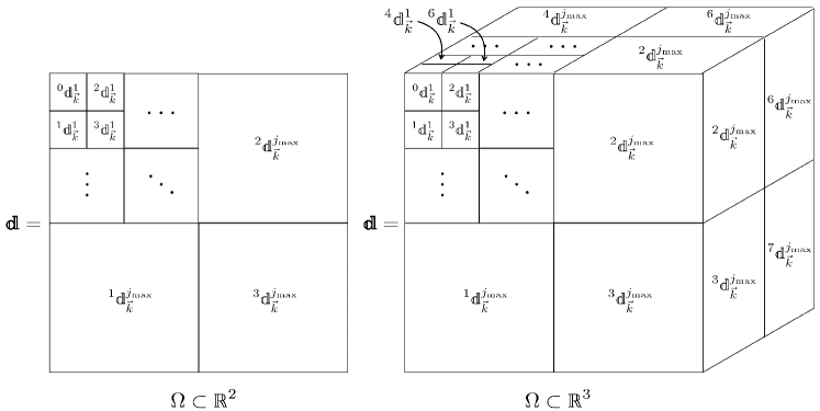
where $\mathbbb{d}$ is an $N$ -dimensional array of wavelet coefficients and $\mathbf{\Psi}(\vec{x})$ is an $N$ -dimensional array of wavelet basis functions. Figure 1 illustrates $\mathbbb{d}$ in $2$ D and $3$ D settings and shows how the notation has been simplified in Eq. 14 as these arrays have a unique index $\vec{m}$ for every $j$ , $\lambda$ , and $\vec{k}$ through the mapping

\displaystyle m_{i}(j,\lambda,\vec{k})=k_{i}+\mathrm{bin}(\lambda)_{i}\times(p\ 2^{j}+1).

(15)

Refer to caption — Figure 1: Array of $\mathbbb{d}$ in $2$ D and $3$ D settings.

With $\vec{x}\in\mathbb{R}^{3}$ , the $3$ D representation of $f(\vec{x})$ given by Eq. 8 and its inverse become

\displaystyle\mathbb{d}_{m_{1}m_{2}m_{3}}=\mathbb{F}_{m_{1}n_{1}}\ \mathbb{F}_{m_{2}n_{2}}\ \mathbb{F}_{m_{3}n_{3}}\ f_{n_{1}n_{2}n_{3}}\qquad\mathrm{and}\qquad f_{m_{1}m_{2}m_{3}}=\mathbb{B}_{m_{1}n_{1}}\ \mathbb{B}_{m_{2}n_{2}}\ \mathbb{B}_{m_{3}n_{3}}\ \mathbb{d}_{n_{1}n_{2}n_{3}},

(16)

on each level $j$ , where $\boldsymbol{f}$ is a $3$ D array of field values. The application of the $\mathbbb{F}$ operators is sometimes called a forward wavelet transform (FWT) or wavelet analysis, whereas application of the $\mathbbb{B}$ operators is sometimes called a backward wavelet transform (BWT) or wavelet synthesis [91, 109]. These matrices are sparse, banded, and constant in time. Due to these properties, the $\mathbbb{F}$ and $\mathbbb{B}$ matrices are never fully assembled, and only nonredundant nonzero entries are stored in memory. Therefore, the FWT and BWT operations have a matrix-free computational implementation.

2.3 Wavelet derivatives

Additionally, the evaluation of spatial derivatives must be defined in order to approximate the solution of PDEs. The Deslauriers-Dubuc wavelet family is continuous and differentiable, with the smoothness of the basis analyzed in [110] and summarized in [105, 106]. This continuity allows the spatial derivative operator to act directly on the basis functions

\displaystyle\frac{\partial^{\alpha}}{\partial x_{i}^{\alpha}}f(\vec{x})

\displaystyle\approx\frac{\partial^{\alpha}}{\partial x_{i}^{\alpha}}\bigg{(}\mathbbb{d}_{m_{1}\ldots\ m_{N}}\ \mathbf{\Psi}(\vec{x})_{m_{1}\ldots\ m_{N}}\bigg{)}=\mathbbb{d}_{m_{1}\ldots\ m_{N}}\frac{\partial^{\alpha}\mathbf{\Psi}(\vec{x})_{m_{1}\ldots\ m_{N}}}{\partial x_{i}^{\alpha}}.

(17)

As in [79], we project the spatial derivative of the basis back onto the wavelet basis and this combination of differentiation and projection transforms Eq. 17 into

\displaystyle\frac{\partial^{\alpha}}{\partial x_{i}^{\alpha}}f(\vec{x})

\displaystyle\approx{}^{(\alpha,i)}\mathbb{D}_{m_{1}\ldots\ m_{N}}^{n_{1}\ldots\ n_{N}}\ \mathbbb{d}_{n_{1}\ldots\ n_{N}}\ \mathbf{\Psi}(\vec{x})_{m_{1}\ldots\ m_{N}},

(18)

where the operator ${}^{(\alpha,i)}\mathbbb{D}$ is defined in terms of “connection coefficients” that result from evaluating the integral

\displaystyle{}^{(\alpha,i)}\mathbb{D}_{\lambda,j,\vec{k}}^{\beta,r,\vec{l}}

\displaystyle=\int\frac{\partial^{\alpha}}{\partial x_{i}^{\alpha}}\bigg{(}{}^{\beta}\Psi_{\vec{l}}^{r}(\vec{x})\bigg{)}\ {}^{\lambda}\widetilde{\Psi}_{\vec{k}}^{j}(\vec{x})\ \mathrm{d}\vec{x},

(19)

for all possible combinations of $\beta,\lambda,r,j\in\mathbb{Z}$ present in the multidimensional wavelet discretization. Much like the integrals in Eq. 8, leveraging the properties of wavelet basis functions allows the integrals in Eq. 19 to be solved exactly and expressed in terms of eigenvector solutions and the four types of filter coefficients (i.e., $h,\ \widetilde{h},\ g,$ and $\widetilde{g}$ ). Application of the ${}^{(\alpha,i)}\mathbbb{D}$ operator results in a discrete approximation of the $\alpha^{\mathrm{th}}$ order derivative in the $i$ -direction with the spatial error

\displaystyle\bigg{|}\bigg{|}\frac{\partial^{\alpha}f}{\partial x_{i}^{\alpha}}

\displaystyle-\frac{\partial^{\alpha}f_{j}}{\partial x_{i}^{\alpha}}\bigg{|}\bigg{|}_{\infty}\leq\mathcal{O}\left(\varepsilon^{1-\frac{\alpha}{p}}\right).

(20)

Note that Eq. 20 reflects the error of the dense $f_{j}$ discretization and not the sparse $f_{\varepsilon}$ discretization since the derivation from [105] assumes a dense grid up to level $j_{\mathrm{max}}$ . Details on how to apply the ${}^{(\alpha,i)}\mathbbb{D}$ operator can be found in A. Much like the $\mathbbb{F}$ and $\mathbbb{B}$ operators, the $\mathbbb{D}$ operator is also sparse and constant in time. Therefore it too has a mostly matrix-free computational implementation which leverages recurrence patterns to compress the memory requirements.

2.4 Nonlinear operations

In order to numerically solve nonlinear PDEs, the discrete analogs of nonlinear operations must be well defined. This would be computationally expensive to perform in the wavelet representation because it requires a convolution operation. Instead, inspired by pseudo-spectral solvers, this work performs nonlinear operations point-wise in the physical domain. Specifically, for each nonlinear operation, a BWT maps the wavelet coefficients to their corresponding field values. Then, the nonlinear operation is approximated by acting on field values at each collocation point. Finally, a FWT of the result returns each collocation point to the wavelet domain. While this approach is more computationally efficient, it introduces aliasing errors. An estimate of the magnitude of such errors is provided in [95], where it is shown that this process approximates the product of fields, $f(\vec{x})$ and $g(\vec{x})$ , with the spatial error

\displaystyle||f(\vec{x})\times g(\vec{x})-f_{\varepsilon}(\vec{x})\times g_{\varepsilon}(\vec{x})||_{\infty}\leq\mathcal{O}(\varepsilon).

(21)

3 Multiresolution wavelet toolkit

This section outlines the multiresolution wavelet toolkit (MRWT), an algorithm designed to numerically approximate the solution to systems of nonlinear PDEs using a sparse discretization with adaptivity and error control. To illustrate the process, consider a general initial-boundary value problem on a finite domain $\Omega\subset\mathbb{R}^{3}$

$\displaystyle\frac{\partial\vec{u}}{\partial t}$	$\displaystyle=\mathcal{F}\left(\vec{x},t,\vec{u},\frac{\partial^{\alpha}\vec{u}}{\partial x_{i}^{\alpha}}\right)\ \mathrm{in}\ \Omega\times[0,T],$
$\displaystyle\vec{u}$	$\displaystyle=\{u_{1}^{0},u_{2}^{0},u_{3}^{0}\}\ \mathrm{in}\ \Omega\times(t=0),$
$\displaystyle\vec{u}$	$\displaystyle=\vec{u}_{d}\ \mathrm{on}\ \partial\Omega_{d}\times[0,T],$
$\displaystyle\frac{\partial^{\alpha}\vec{u}}{\partial x_{i}^{\alpha}}$	$\displaystyle=\vec{u}_{n}\ \mathrm{on}\ \partial\Omega_{n}\times[0,T].$	(22)

The order of the PDE sets requirements on the continuity of the wavelet basis, influencing the wavelet order $p$ . Once $p$ is set, fields and their spatial derivatives are projected onto the wavelet basis functions using Eq. 14 and Eq. 18. During this initialization phase, MRWT precomputes the nonredundant entries in the $\mathbbb{F}$ , $\mathbbb{B}$ , and ${}^{(\alpha,i)}\mathbbb{D}$ operators. This process transforms the nonlinear PDE into a nonlinear ODE

\displaystyle\frac{\mathrm{d}\vec{u}_{\varepsilon}}{\mathrm{d}t}=\mathcal{F}_{\varepsilon}\left(\vec{x},t,\vec{u}_{\varepsilon}\right).

(23)

Each scalar component of the initial condition (i.e., $u_{1}^{0}$ , $u_{2}^{0}$ , and $u_{3}^{0}$ ) is projected individually onto the wavelet basis one resolution level at a time, starting from the coarsest resolution. All wavelet coefficients on $j=1$ are calculated and each point of type $\lambda=0$ or with a magnitude greater than or equal to a user-prescribed threshold $\varepsilon$ is deemed essential. The set of essential points for a particular scalar (e.g., $u_{1}$ ) is defined by

\displaystyle\mathbb{E}_{\bullet}=\left\{\vec{x}\in\Omega:\left[\left|{}^{0}\mathbb{d}_{\vec{k}}^{1}(\bullet)\right|\geq 0\;\vee\;\left|{}^{\lambda}\mathbb{d}_{\vec{k}}^{j}(\bullet)\right|\geq\varepsilon\right],\;j\in[1,j_{\mathrm{max}}],\;\lambda\in[1,7],\;\vec{k}\in\mathbb{Z}\right\},

(24)

where $\bullet$ is a marker for a particular scalar field. The set $\mathbb{E}_{\bullet}$ is populated on higher resolution levels through exploring spatial regions near the already discovered essential points. Identifying and calculating all essential points for a particular scalar creates a sparse multiresolution spatial discretization without generating dense grids of uniform spacing. This process is repeated for each scalar component of the initial condition (i.e., $\mathbb{E}_{u_{1}}$ , $\mathbb{E}_{u_{2}}$ , and $\mathbb{E}_{u_{3}}$ ). Furthermore, according to Eq. 13, the spatial accuracy of the initial condition is known a priori to be $\mathcal{O}\left(\varepsilon\right)$ .

Since the solution of the PDE may advect and evolve over time, the points which are presently essential $\mathbb{E}^{n}$ (where $n$ is the current time step) may not be same collection of points which are essential in future times (e.g., $\mathbb{E}^{n+1}$ ). Therefore, MRWT uses a predictor-corrector strategy to predict where new collocation points will be required and corrects that prediction during temporal integration until the necessary grid is obtained at each time step. A trial grid is defined for each scalar by including points in the neighborhood of that scalar’s essential points such that

\displaystyle\mathbb{T}_{\bullet}

\displaystyle=\bigcup_{\forall\vec{y}\in\mathbb{E}_{\bullet}}\left\{\vec{x}\in\Omega:\left|y_{i}-x_{i}\right|<\frac{b_{i}-a_{i}}{p\ 2^{r}},\;i\in[1,3],\;j\in[r,\min(r+1,j_{\mathrm{max}})]\right\},

(25)

where the level $r$ is obtained from the coordinate of the essential point $\vec{y}\in\mathbb{E}_{\bullet}$ using the inverse mapping from Section 2.2.

Next, the ${}^{(\alpha,i)}\mathbbb{D}$ operator is used to identify which points influence the derivative calculations at each point in the trial grid $\mathbb{T}$ . As shown in A, the wavelet derivative operator is a multiresolution weighted sum. Calculating a wavelet coefficient corresponding to a spatial derivative on resolution level $r$ will involve contractions with points below, above, and on level $r$ . However, because the grid is sparse, many of the collocation points involved in the application of the ${}^{(\alpha,i)}\mathbbb{D}$ operator, given by Eq. 19 may be absent. This affects the validity of the error estimate in Eq. 20 as its derivation assumes complete stencils on each resolution level with $f_{j}(\vec{x})$ given by Eq. 9. Since attempting to complete stencils on all levels $j\in[1,j_{\mathrm{max}}]$ for all points would lead to dense grids of uniform spacing (i.e., $f_{j}(\vec{x})$ in Eq. 9), the MRWT algorithm completes derivative stencils for each point in each scalar’s trial grid up to its own level $r$ according to

\displaystyle\mathbb{G}_{\bullet}

\displaystyle=\bigcup_{\forall\vec{y}\in\mathbb{T}_{\bullet}}\left\{\vec{x}\in\Omega:\left[\vec{x}=\vec{y}\;\vee\;\left|{}^{\lambda}_{\beta}\mathbb{D}^{j,\vec{k}}_{r,\vec{l}}\right|>0\right],\;j\leq r,\;\lambda\in[0,7],\;\vec{k}\in\mathbb{Z}\right\},

(26)

where the type $\beta$ , level $r$ , and index $\vec{l}$ are obtained from the coordinate of the point $\vec{y}\in\mathbb{T}_{\bullet}$ using the inverse mapping from Section 2.2.

For each scalar in the system of PDEs, the algorithm constructs $\mathbb{E}_{\bullet}\subset\mathbb{T}_{\bullet}\subset\mathbb{G}_{\bullet}$ and the sparse multiresolution computational grid defined by $\mathbb{G}=\mathbb{G}_{u_{1}}\cup\mathbb{G}_{u_{2}}\cup\mathbb{G}_{u_{3}}$ . The grid, $\mathbb{G}_{\bullet}$ contains all of the collocation points that are required to resolve that particular field and its derivatives at discrete times $n$ and $n+1$ , with the spatial accuracy bound by Eqs. 13 and 21 and approximated by Eq. 20. However, due to overlap between the sets from different scalars, the computational grid may contain more data than is needed for a given scalar. This is corrected by zeroing extraneous coefficient values

\displaystyle{}^{\lambda}\mathbb{d}_{\vec{k}}^{j}(\bullet)=0\;\forall\ \vec{x}\in\mathbb{G}\setminus\mathbb{G}_{\bullet},

(27)

where the type $\lambda$ , level $j$ , and index $\vec{k}$ are obtained from the coordinate of the point $\vec{x}$ using the inverse mapping from Section 2.2. Equations 24, 25, 26 and 27 completely define the spatial discretization used to solve systems of nonlinear PDEs. Leveraging wavelet theory from Section 2 to construct the sets $\mathbb{E},\mathbb{T},$ and $\mathbb{G}$ using the wavelet derivative operator $\mathbb{D}$ is one of the novelties of our work. As we show later, this grid construction is necessary to control the spatial accuracy.

An explicit, embedded, Runge-Kutta time integration scheme [111] is used to progress the solution from the time step $n$ to a trial time step $(n+1)^{*}$ . This converts the ODE in Eq. 23 into a system of algebraic equations which update $\vec{u}_{\varepsilon}^{\ n}$ to the trial time step $\vec{u}_{\varepsilon}^{\ (n+1)^{*}}$ while providing an estimate of the temporal error and adjusting the time-step size $\Delta t$ such that the temporal error is less than the user prescribed value. In this work, we set the tolerance to be an order of magnitude less than the spatial error epsilon (i.e., $\mathrm{tol}=\varepsilon/10$ ) and adapt the time-step size according to

\displaystyle\Delta t_{\mathrm{new}}=\Delta t\left(\frac{\mathrm{tol}}{\|\vec{u}^{\ n+1}_{K+1}-\vec{u}^{\ n+1}_{K}\|_{\infty}}\right)^{\frac{1}{K+1}},

(28)

where $K$ is the order of the method used to advance $n\rightarrow(n+1)^{*}$ . Furthermore, similar to the work done by [112], we prevent the time-step size from varying too abruptly by bounding the suggested $\Delta t_{\mathrm{new}}$ such that

\displaystyle\Delta t-10\%\Delta t\leq\Delta t_{\mathrm{new}}\leq\Delta t+0.1\%\Delta t.

(29)

At each intermediate stage of the Runge-Kutta integration, no boundary conditions are enforced in order to preserve high order temporal convergence [113]. At the final stage of the Runge-Kutta integration, once the PDE solution has evolved to the trial time $(n+1)^{*}$ , boundary conditions are enforced directly (i.e., for Dirichlet data) or by using the penalty formulation [114] that will modify Eq. 23 on the boundary (i.e., for Dirichlet and/or Neumann data).

The magnitudes of the wavelet coefficients at the new time will determine if the grid prediction must be corrected. A list of corrections is defined as the set difference between the essential points at the trial time step and the essential points at the current time

\displaystyle\mathbb{C}^{n}

\displaystyle=\mathbb{E}^{(n+1)^{*}}\ \setminus\ \mathbb{E}^{n},

(30)

If the list of corrections contains any points then these corrections are added to the list of existing essential points

\displaystyle\mathbb{E}^{n}=\mathbb{E}^{n}\ \cup\ \mathbb{C}^{n}.

(31)

In this case, the trial time step is discarded and the computational grid at time step $n$ is supplemented with new collocation points to obtain new $\mathbb{T}^{n}_{\bullet}$ and new $\mathbb{G}^{n}_{\bullet}$ according to Eqs. 25 and 26. The value of the wavelet coefficients stored at these new points is set to zero at time step $n$ . After correcting the grid, a new trial time step is performed and Eqs. 30 and 31 are re-evaluated. This process of predicting and correcting is repeated iteratively until the list of corrections is an empty set. This grows the sparse computational grid as it evolves with the solution of the PDE such that the spatial error is bounded by Eqs. 13 and 21 and approximated by Eq. 20 at each time step.

When the trial time step is accepted (i.e., $\mathbbb{d}^{n+1}=\mathbbb{d}^{(n+1)^{*}}$ ) some wavelet coefficients are no longer needed. Collocation points at the new time are retained only if they are deemed essential (i.e., Eq. 24), part of the trial grid (i.e., Eq. 25), or needed to complete the derivative stencil (i.e., Eq. 26). This procedure prunes the sparse computational grid as it evolves with the solution of the PDE.

MRWT has been implemented as a hybrid MPI+OpenMP framework using modern C++. The multidimensional sparse geometry is stored in sorted coordinate-object format (COO) and is replicated across ranks. Corresponding collocated scalar field data is distributed linearly across ranks and stored in struct-of-array form. This design permits temporal and spatial locality for sparse stencil contractions as well as vectorizable data parallelism for point-wise, right-hand-side kernels. The predictor-corrector algorithm performs bulk insertion and deletion of points relatively infrequently resulting in periodic merge and sort operations. Communication includes both point-to-point messaging and global collectives, and rebalancing is performed after each time step in which the geometry changes. The $\mathbbb{F}$ and $\mathbbb{B}$ stencil operators are matrix-free while ${}^{(\alpha,i)}\mathbbb{D}$ is optimally compressed (i.e., the operator is precomputed, stored sparsely, and its evaluation is carefully scheduled to amortize costs). Preliminary scaling results for the framework appear in B.

3.1 Code verification

Suppose the generic initial-boundary value problem in Section 3, is specified to be the nonlinear quasi- $2$ D Burgers’ equation

\displaystyle\frac{\partial u}{\partial t}+(u+c)\left[\frac{\partial u}{\partial x_{1}}\cos{(\theta)}+\frac{\partial u}{\partial x_{2}}\sin{(\theta)}\right]

\displaystyle=\nu\left[\frac{\partial^{2}u}{\partial x_{1}^{2}}\cos{{}^{2}(\theta)}+\frac{\partial^{2}u}{\partial x_{1}\partial x_{2}}\sin{(2\theta)}+\frac{\partial^{2}u}{\partial x_{2}^{2}}\sin{{}^{2}(\theta)}\right],

(32)

where $\theta$ is a specified constant angle of rotation, projecting the $1$ D Burgers’ equation into a second spatial dimension. Two analytical solutions exist distinguished by their initial conditions and the value of $c$ . In both cases, the boundary conditions are Dirichlet defined by the respective analytical solutions with the following parameters

\displaystyle\vec{x}

\displaystyle\in[-1,1]^{2},

\displaystyle t

\displaystyle\in[0,1/2],

\displaystyle\theta

\displaystyle\in[0,\pi/2],

\displaystyle\nu

\displaystyle=10^{-2}.

(33)

First, for $c=0$

	$\displaystyle u_{0}$	$\displaystyle=-\sin{(x_{1}\pi\cos{\theta}+x_{2}\pi\sin{\theta})},$
	$\displaystyle u(\vec{x},t)$	$\displaystyle=-\frac{\int\sin(\pi x_{1}\cos(\theta)+\pi x_{2}\sin(\theta)-\pi\eta)\ \exp\left(\frac{-\cos(\pi x_{1}\cos(\theta)+\pi x_{2}\sin(\theta)-\pi\eta)}{2\pi\nu}\right)\ \exp\left(\frac{-\eta^{2}}{4\nu t}\right)\mathrm{d}\eta}{\int\exp\left(\frac{-\cos(\pi x_{1}\cos(\theta)+\pi x_{2}\sin(\theta)-\pi\eta)}{2\pi\nu}\right)\ \exp\left(\frac{-\eta^{2}}{4\nu t}\right)\mathrm{d}\eta}.$		(34)

The MRWT solution of Section 3.1 can be obtained at early times with a coarse grid, but requires increasingly higher resolution as the gradients become more extreme over time. This formulation verifies MRWT’s ability to dynamically refine the sparse multiresolution spatial discretization.

Alternatively, for $c\neq 0$

	$\displaystyle u_{0}$	$\displaystyle=-\tanh{[((x_{1}+0.5)\cos{\theta}+(x_{2}+0.5)\sin{\theta})/2\nu]},$
	$\displaystyle u(\vec{x},t)$	$\displaystyle=-\tanh{\left(\frac{(x_{1}+0.5)\cos{(\theta)}+(x_{2}+0.5)\sin{(\theta)}-ct}{2\nu}\right)}.$		(35)

The MRWT solution of Section 3.1 requires high resolution only in the vicinity of the steep feature that advects through the spatial domain over time. This formulation verifies MRWT’s ability to insert and remove collocation points to resolve evolving features (e.g., shocks).

The MRWT algorithm has been used with the embedded $\mathcal{O}(\Delta t^{4})$ and $\mathcal{O}(\Delta t^{5})$ explicit Runge-Kutta method developed in [111] to solve Eq. 32 for a variety of angles $\theta$ . The numerical solution has been compared to the analytical solutions from Sections 3.1 and 3.1 to evaluate the error at each time step. Figure 2 shows that the error in the solution is bounded regardless of the angle $\theta$ and the error is comparable to the one-dimensional analog of Eq. 32. Note that there is no distinction in the measured errors between the $0^{\circ}$ and $90^{\circ}$ or the $30^{\circ}$ and $60^{\circ}$ rotations, since these solutions are reflections across the $x_{1}=x_{2}$ plane.

Additionally, the solution to both versions of Eq. 32 with $\theta=30^{\circ}$ , $p=6$ , and $\varepsilon=10^{-2}$ is shown at various times in Fig. 3 demonstrating that the sparse dynamically adaptive grid provides resolution only where and when it is needed to track features as they develop or move through the domain.

Furthermore, the analytical solutions of Sections 3.1 and 3.1 have been used to evaluate the error and corresponding convergence rate of the algorithm by solving Eq. 32 for a range of $\varepsilon$ and $p$ values. Figure 4 shows the convergence rates calculated half-way through the simulation time with $\theta=30^{\circ}$ , which are in agreement with the theoretical estimates from Eqs. 13, 21 and 20. In particular, the order of error for the nonlinear PDE should be between $\mathcal{O}(\varepsilon^{1-\frac{\alpha}{p}})$ and $\mathcal{O}(\varepsilon)$ . Results presented in Fig. 4 retain these properties.

In order to test MRWT’s ability to solve systems of equations, canonical Navier-Stokes examples such as the Sod shock tube and a Taylor-Sedov blast wave have been presented in [105, 106, 115]. C contains analysis of $1$ D, $2$ D, and $3$ D simulations of the Taylor-Sedov blast wave. Additional verification of the MRWT algorithm is provided by comparing the location of the simulated shock wave to the theoretical prediction from [116].

4 Nonlinear dynamic damage modeling

Having verified the mathematical correctness of the MRWT algorithm, we now demonstrate the multiscale capabilities by modeling high-strain rate damage nucleation and propagation in nonlinear solids. The following subsections will outline the continuum formulation of finite strain kinematics and the constitutive description provided by damage mechanics. Since this work leverages wavelet basis functions for the computational implementation, all governing equations will be defined in the Eulerian frame.

4.1 Governing equations

Let a body in a reference configuration $\mathcal{B}_{0}\subset\mathbb{R}^{3}$ be defined by a continuum of material points (i.e., particles $\vec{X}\in\mathcal{B}_{0}$ ). After some time $t\in[0,T]$ , the body is in a deformed configuration where $\varphi:\mathcal{B}_{0}\times[0,T]\rightarrow\mathbb{R}^{3}$ defines the motion that maps particles to their positions $\vec{x}=\varphi(\vec{X},t)$ (i.e., places) in the current configuration $\mathcal{B}(t)=\varphi(\mathcal{B}_{0},t)$ . The mechanical effects are governed by the conservation of linear momentum in the Eulerian frame $\Omega\subset\mathcal{B}(t)\subset\mathbb{R}^{3}$

$\displaystyle\rho\dot{\vec{v}}$	$\displaystyle=\nabla\cdot\boldsymbol{\sigma}+\rho\vec{b},\ \mathrm{in}\ \Omega\times[0,T],$
$\displaystyle\vec{v}$	$\displaystyle=\vec{v}_{0}\ \mathrm{in}\ \Omega\times(t=0),$
$\displaystyle\vec{v}$	$\displaystyle=\vec{v}_{d}\ \mathrm{on}\ \partial\Omega_{d}\times[0,T],$
$\displaystyle\frac{\partial^{\alpha}\vec{v}}{\partial x_{i}^{\alpha}}$	$\displaystyle=\vec{v}_{n}\ \mathrm{on}\ \partial\Omega_{n}\times[0,T],$	(36)

where $\rho(\vec{x},t)$ is the density, $\boldsymbol{\sigma}(\vec{x},t)$ is the Cauchy stress tensor, and $\vec{b}(\vec{x},t)$ is a body force per unit mass.

Inspired by the reference map technique [38], the inverse mapping $\vec{X}=\varphi^{-1}(\vec{x},t)$ is used to determine which particles occupy specified spatial coordinates (i.e., places $\vec{x}$ ). However, instead of keeping track of the reference map $\varphi^{-1}(\vec{x},t)$ directly, we model the displacement $\vec{u}(\vec{x},t)=\vec{x}-\vec{X}$ , and like in [38] we derive the associated evolution equation from $\dot{\vec{X}}=\vec{0}$

$\displaystyle\dot{\vec{u}}$	$\displaystyle=\vec{v},\ \mathrm{in}\ \Omega\times[0,T],$
$\displaystyle\vec{u}$	$\displaystyle=\vec{u}_{0}\ \mathrm{in}\ \Omega\times(t=0),$
$\displaystyle\vec{u}$	$\displaystyle=\vec{u}_{d}\ \mathrm{on}\ \partial\Omega_{d}\times[0,T],$
$\displaystyle\frac{\partial^{\alpha}\vec{u}}{\partial x_{i}^{\alpha}}$	$\displaystyle=\vec{u}_{n}\ \mathrm{on}\ \partial\Omega_{n}\times[0,T].$	(37)

To finalize the Lagrangian-Eulerian coupling of Sections 4.1 and 4.1, we use the conservation of mass in the Lagrangian frame

\displaystyle\rho

\displaystyle=\frac{\rho_{0}}{\mathrm{J}},\mathrm{in}\ \Omega_{0}\times[0,T],

(38)

where $\rho_{0}(\vec{X})$ is the density in the reference configuration, $\mathrm{J}(\vec{X},t)=1/\det{\mathbf{f}}$ is the Jacobian of the deformation, $\mathbf{f}(\vec{x},t)=\boldsymbol{1}-\nabla\vec{u}$ is the inverse deformation gradient, and $\boldsymbol{1}$ is the second order identity tensor.

4.2 Constitutive theory

The constitutive relations are derived from a thermodynamically consistent description with an energy-based isotropic damage model, applicable under finite strains. In this work, the following potentials describe the strain energy density (per reference volume) and the Helmholtz specific energy

\displaystyle W(\omega,\boldsymbol{b})

\displaystyle=(1-\omega)\left[\underbrace{\frac{\kappa}{2}\left(e^{(\mathrm{J}-1)}-\ln(\mathrm{J})-1\right)}_{\text{volumetric}}+\underbrace{\frac{\mu}{2}\left(\mathrm{J}^{-\frac{2}{3}}\mathrm{tr}(\boldsymbol{b})-3\right)}_{\text{deviatoric}}\right],

\displaystyle\psi(\omega,\boldsymbol{b})

\displaystyle=\frac{1}{\rho_{0}}W(\omega,\boldsymbol{b}),

(39)

where $\boldsymbol{b}(\vec{x},t)$ is the left Cauchy-Green strain tensor defined through its inverse $\boldsymbol{b}^{-1}(\vec{x},t)=\mathbf{f}^{T}\mathbf{f}$ , $\kappa$ is the bulk modulus, $\mu$ is the shear modulus, and $\omega\in[0,1]$ is the scalar damage variable.

Neglecting all but mechanical effects, the second Law of Thermodynamics has the form

\displaystyle\rho\dot{\psi}-\boldsymbol{\sigma}:\nabla\vec{v}\leq 0.

(40)

Combining Eq. 40 with Eq. 39 yields

\displaystyle\mathcal{D}_{\omega}=Y\ \dot{\omega}

\displaystyle\geq 0,

\displaystyle\boldsymbol{\sigma}

\displaystyle=2\rho\frac{\partial\psi}{\partial\boldsymbol{b}}\cdot\boldsymbol{b},

(41)

where $Y(\vec{x},t)=-\rho\ \partial\psi/\partial\omega$ is the damage energy release rate (thermodynamic force conjugate to the damage variable $\omega$ ) and $\mathcal{D}_{\omega}$ is the damage dissipation. From Eqs. 39 and 41 the Cauchy stress becomes

\displaystyle\boldsymbol{\sigma}

\displaystyle=(1-\omega)\ \left[\frac{\kappa}{2}\left(e^{(\mathrm{J}-1)}-\frac{1}{\mathrm{J}}\right)\boldsymbol{1}+\mu\ \mathrm{J}^{-5/3}\ \boldsymbol{b}^{\prime}\ \right],

(42)

where $\boldsymbol{b}^{\prime}(\vec{x},t)$ is the deviatoric part of $\boldsymbol{b}(\vec{x},t)$ .

The evolution of the damage variable $\omega$ is derived in a similar fashion as in plasticity, [62, 39, 64, 40, 41, 63] First, an energy-based damage criterion is defined by

\displaystyle g(Y,\chi)

\displaystyle=G(Y)-\chi\leq 0.

(43)

The internal state variable $\chi\in[0,1]$ sets the threshold for how much energy is required in order to increase the amount of damage in the material. The function $G(Y)\in[0,1]$ models the damage process. In this work, it is defined as the Weibull distribution

\displaystyle G(Y)

\displaystyle=1-\exp{\left[-\left(\frac{Y-Y_{\mathrm{in}}}{p_{1}Y_{\mathrm{in}}}\right)^{p_{2}}\right]},

(44)

though alternative definitions are admissible (e.g., [6, 117, 42, 43]). The material parameter $Y_{\mathrm{in}}$ is the energy barrier required to initiate damage and the parameters $p_{1}$ and $p_{2}$ are scale and shape parameters, which facilitate modeling a wide range of material behaviors.

The irreversible dissipative damage evolves according to two evolution equations

\displaystyle\dot{\omega}

\displaystyle=\dot{\varkappa}\frac{\mathrm{d}G(Y)}{\mathrm{d}Y},

\displaystyle\dot{\chi}

\displaystyle=\dot{\varkappa}\frac{\mathrm{d}G(Y)}{\mathrm{d}Y},

(45)

where $\dot{\varkappa}=\dot{Y}$ is a damage consistency parameter determined by enforcing the consistency condition $\dot{g}=0$ . The damage loading and unloading are described by the Kuhn-Tucker complimentary conditions

\displaystyle\dot{\varkappa}

\displaystyle\geq 0,

\displaystyle g(Y,\chi)

\displaystyle\leq 0,

\displaystyle\dot{\varkappa}\ g(Y,\chi)

\displaystyle=0.

(46)

There are well-posedness and uniqueness problems associated with Eq. 45 which lead to numerical results that do not converge with respect to the spatial discretization. In order to maintain material ellipticity, nonlocal models [9] or viscous regularization [118] can be introduced. In this work, a rate dependent viscous damage model is obtained by replacing Eq. 45 with

\displaystyle\dot{\omega}

\displaystyle=\mu_{\omega}\ \langle\phi(g)\rangle,

\displaystyle\dot{\chi}

\displaystyle=\mu_{\omega}\ \langle\phi(g)\rangle,

(47)

where $\mu_{\omega}$ is the damage viscosity, $\phi(g)$ is the damage flow function, and $\langle\bullet\rangle$ are McAuley brackets. Assuming a linear flow function (i.e., $\phi(g)=g$ ), the Eulerian description for the damage evolution equations becomes

\displaystyle\frac{\partial\omega}{\partial t}

\displaystyle=-\nabla\omega\cdot\vec{v}+\mu_{\omega}\ \langle G(Y)-\chi\rangle,

\displaystyle\frac{\partial\chi}{\partial t}

\displaystyle=-\nabla\chi\cdot\vec{v}+\mu_{\omega}\ \langle G(Y)-\chi\rangle.

(48)

This Eulerian-Lagrangian continuum model for the high-strain rate damage and its numerical implementation using the wavelet solver described in Section 3 is one of the novelties of this work.

5 Numerical results

This section presents results from modeling high-strain rate damage under finite strains using equations from Section 4 and the numerical method from Section 3. Specifically Sections 4.1 and 4.1 model the motion of material in the Eulerian frame, Eq. 38 provides a kinematically consistent density, and is closed by the stress description in Eq. 42 and the damage evolution in Eq. 48. Table 2 lists the parameters used to model PMMA [119] with a peak stress $\sigma_{\mathrm{max}}\approx 100$ MPa and an energy release rate $G_{I}\approx 350$ J/m². These values are consistent with experimental measurements provided in [120]. We note that the viscous damage model introduces the characteristic damage length scale $l_{\omega}\propto c_{l}/\mu_{\omega}$ , where $c_{l}=\sqrt{E/\rho_{0}}$ is the longitudinal wave speed and $E$ is Young’s modulus [41, 63]. In this work, we set the damage viscosity $\mu_{\omega}$ such that the damage length scale is consistent with material data (i.e., $l_{\omega}\approx\mathcal{O}(100\mu$ m)) [121].

Table 2: Model parameters for dynamic damage of PMMA.

Variable	Name	Value
$\rho_{0}$	Density	$1183\ \mathrm{kg/m}^{3}$
$\kappa$	Bulk modulus	$5.86\ \mathrm{GPa}$
$\mu$	Shear modulus	$2.29\ \mathrm{GPa}$
$\mu_{\omega}$	Damage viscosity	$10^{7}\ \mathrm{1/s}$
$Y_{\mathrm{in}}$	Initiation threshold	$6\times 10^{4}\ \mathrm{J/m}^{3}$
$p_{1}$	Scale parameter	$30$
$p_{2}$	Shape parameter	$1.01$

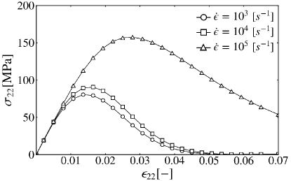
Figure 5 shows the rate-dependant stress-strain response using material parameters from Table 2 in a uniaxial tension setting. These results are consistent with experimental measurements of PMMA exhibiting higher peak tensile strength under dynamic loading [122] with strain rate effects [123].

A model of mode-I fracture under plane-strain deformation is defined through the initial conditions

\displaystyle\vec{v}(\vec{x},0)

\displaystyle=\{0,\dot{\epsilon}\ x_{2},0\},

\displaystyle\vec{u}(\vec{x},0)

\displaystyle=\vec{0},

\displaystyle\rho(\vec{x},0)

\displaystyle=\rho_{0},

(49)

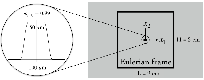
with a high strain rate of $\dot{\epsilon}=5,000$ s^-1. Figure 6 depicts the Eulerian domain, defined by a $2$ cm square, containing an initial flaw proportional to the characteristic length of viscous damage (i.e., $\mathcal{O}(100\ \mu$ m)).

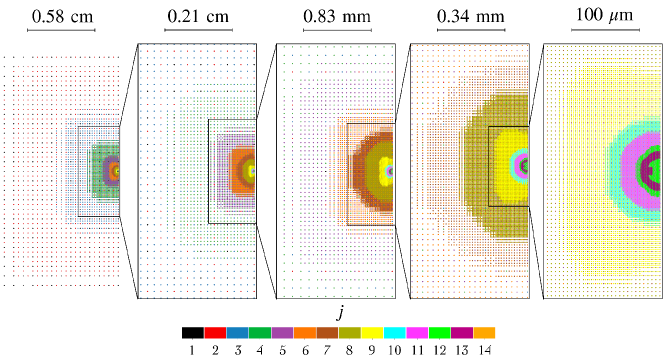
In this example, the sparse multiresolution spatial discretization was restricted to no more than $J=14$ resolution levels which provides continuous resolution between $\mathcal{O}(100\ \mathrm{nm})$ on the finest level and $\mathcal{O}(1\ \mathrm{cm})$ on the overall domain (i.e., $\mathcal{O}(10^{5})$ range of length-scales). This range of spatial resolution is impressive in the context of damage simulations as many other solution strategies are either limited to small domains or discretize on a scale that is unable to resolve the characteristic crack thickness (e.g., typical simulations have a range of length-scales around $\mathcal{O}(10^{1})$ [124, 125] or $\mathcal{O}(10^{2})$ [126, 41, 63]).

The remaining figures in this section display simulation results only on the half-domain, obtained from running on $960$ cores. While the embedded Runge-Kutta temporal integration provides a dynamic time-step size according to Eqs. 28 and 29, in general $\Delta t\approx\mathcal{O}(10^{-11}\ \mathrm{s})$ requiring approximately $200$ thousand time steps was used to reach $2\ \mu$ s. As shown in Fig. 7, our algorithm adaptively provides resolution only where it is needed as defined by the user-prescribed $\varepsilon$ threshold parameters, which for all results in this section are

\displaystyle\varepsilon_{\omega}

\displaystyle=\varepsilon_{\chi}=10^{-3},

\displaystyle\varepsilon_{\vec{u}}

\displaystyle=10^{-7}\ \mu\mathrm{m},

\displaystyle\varepsilon_{\vec{v}}

\displaystyle=10^{-2}\ \mathrm{m/s}.

(50)

The MRWT discretization provides dynamic compression of the solution to the PDE. For example, with $p=6$ the initial condition is discretized on a sparse grid of $35,689$ collocation points on the full domain, whereas a uniform grid with $J=14$ resolution levels would have $38,655,098,881$ points. Furthermore, this extreme compression continues throughout the simulation where after $2\ \mu$ s of deformation, our sparse multiresolution discretization contains only $810,633$ collocation points on the full domain.

The deformation around the initial flaw induces strain localization as exhibited by the concentrated displacement in Fig. 8. Note that the background displacement of mode-I opening (i.e., $u_{2}^{\mathrm{bg}}\approx v_{2}^{0}\times t$ ) is subtracted from the $u_{2}$ component of displacement to reveal solution features (e.g., pronounced displacement of material points in the vicinity of the flaw).

Figure 9 illustrates the dynamics of this process with significant spikes in the velocity field (e.g., $\mathcal{O}(1)\ \mathrm{m/s}$ ) over a very small region (e.g., $\mathcal{O}(10^{-5})\ \mathrm{m}$ ). Again, the background velocity of mode-I opening (i.e. $v_{2}^{\mathrm{bg}}\approx v_{2}^{0}$ ) is subtracted from the $v_{2}$ component of velocity to reveal solution features (e.g., symmetric local maxima/minima above/below the damage profile).

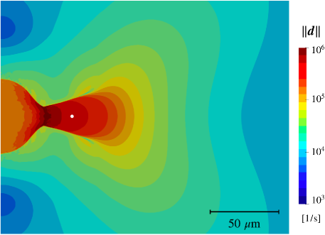
Figure 10 reveals the extreme nature of the rate of the deformation tensor (i.e., $\boldsymbol{d}=(\ \nabla\vec{v}\ )^{\mathrm{sym}}$ ). Since this quantity is proportional to the strain rate, the MRWT simulation suggests that in the damaged regions the material experiences strain rates multiple orders of magnitude higher than the imposed loading rate of $\dot{\epsilon}=5,000\ \mathrm{s}^{-1}$ . This observation is consistent with the model depicted in Fig. 5.

This consideration is made more clear by observing the temporal evolution of stress and strain at a particular coordinate outside the region of the initial flaw (i.e., $\vec{x}=[52\nicefrac{{1}}{{12}},0,0]\ \mu$ m). Figure 11 plots the stress and strain at this location over time. In this figure, the precipitous decline in the stress reflects the brittle nature of PMMA. Furthermore, there are $2$ distinct strain rates separated by the limit point in the stress-strain curve around $t\approx 1.6\ \mu$ s (i.e., $\dot{\epsilon}\approx 10^{4}\ \mathrm{s}^{-1}$ during hardening and $\dot{\epsilon}\approx 3\times 10^{5}\ \mathrm{s}^{-1}$ during softening).

This strain localization around the initial flaw provides the energy to initiate and grow damage in a process zone. Figure 12 shows the damage profile as it evolves and illustrates the dynamic adaptivity of the MRWT spatial discretization. A stress concentration develops in front of the process zone which propagates in a direction orthogonal to the applied deformation. Figures 13 and 11 demonstrate that the damaged material in the wake of the stress concentration has a reduced capacity to support a load and experiences significantly higher strains, reaching approximately $20\%$ .

According to linear fracture mechanics [25], material deformed in this configuration will generate a crack of length $a(t)$ that grows with a speed $\dot{a}(t)$ which accelerates until reaching the Rayleigh speed $c_{R}$ . For the material parameters in Table 2, $c_{R}\approx 1,295$ m/s. An estimate for the length of the crack from the MRWT simulation is provided by measuring the distance from the origin to the peak stress (e.g., Fig. 13). From the initial condition, the crack starts with a nonzero length $a_{0}\approx 46.4\ \mu$ m. After $2.2\ \mu$ s the crack has grown to a length of $a\approx 135.1\ \mu$ m. The corresponding speed of the crack from the MRWT simulation is $\dot{a}\approx 280$ m/s, indicating the early stage of the damage process. The crack speed was computed from the slopes of quadratic functions locally fit to the crack length over time.

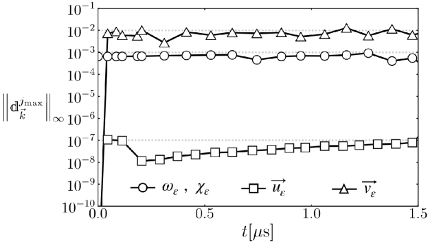
Lastly, our novel numerical method can provide assessment of the quality of the solution (i.e., the solution verification). Whereas traditional numerical techniques require a sequence of solutions on multiple grids, this work provides self-verification from a single simulation. Specifically, with $J=14$ resolution levels available to our algorithm, the error of the solution of the PDEs is bound by Eqs. 13 and 21 and approximated by Eq. 20 as long as $j_{\mathrm{max}}<J$ . Beyond this limit (i.e., $j_{\mathrm{max}}\geq J$ ), our algorithm provides automatic estimates of the error through the magnitude of the wavelet coefficients on the highest resolution level,

\displaystyle\mathrm{error}(\bullet)\propto\left\|{}^{\lambda}\mathbb{d}_{\vec{k}}^{J}(\bullet)\right\|_{\infty}.

(51)

Figure 14 shows the error estimates from the damage simulation for the first $1.5\ \mu$ s with $j_{\mathrm{max}}<J$ . In this time interval, each field has an error proportional to their respective epsilons according to Eq. 50. After $2\ \mu$ s of deformation when $j_{\mathrm{max}}$ was no longer guaranteed, the relative percent error for each field was: $2.7\%$ for the damage variables, $0.027\%$ for the displacement, and $9.7\%$ for the velocity.

6 Conclusions

Our proposed wavelet based algorithm is well suited for computational science and engineering applications requiring dynamic resolution across multiple spatial and temporal scales. Whereas traditional numerical methods require a posteriori remeshing/refining procedures, the wavelet basis functions provide intrinsic adaptivity with resolution only where and when it is needed according to the user-prescribed accuracy. Although other wavelet based solvers have been developed in the past, our novel algorithm is the first to the best of our knowledge which uses the wavelet operators (e.g., the direct differentiation of the wavelet basis) to inform the grid adaption strategy. In this work, the spatial discretization is guided by the wavelet error estimates for fields, derivatives, and nonlinear operations. The error of the solution of the PDE is controlled in space and time by combining the predictor/corrector grid adaption procedure with embedded Runge-Kutta time integration. Furthermore, the matrix formulation of the wavelet operators allows the MRWT algorithm to be trivially applied to $N$ spatial dimensions and data compression is enhanced by using the minimum number of points on the coarse grid, thereby maximizing the number of collocation points which have the potential to be omitted from the discretization. MRWT has been verified by showing spatial convergence of the solution of nonlinear PDEs at rates that are consistent with the aforementioned error estimates. Additionally, the capabilities of MRWT have been demonstrated by simulating multiscale applications, such as the Navier-Stokes equations.

Finally, we have demonstrated our wavelet numerical method on a difficult high-strain rate dynamic damage problem. The sparse multiresolution discretization provides continuous resolution between $O(100\ \mathrm{nm})$ on the finest level and $O(1\ \mathrm{cm})$ on the overall domain. As shown, the simulation of damage nucleation and propagation is well resolved on this discretization spanning $5$ orders of magnitude without imposing significant computational overhead. By providing highly resolved kinematic quantities and associated constitutive response, our algorithm can inform material scientists of the extreme dynamics involved in material failure, thereby facilitating the design of robust materials. Furthermore, since the wavelet algorithm provides accurate simulations of nonlinear dynamic damage it is a convenient tool for the development of more accurate macroscopic damage models (e.g., anisotropic). This work illustrates that our wavelet solver is capable of simulating complex systems with the resolution required to validate material models against experimental results.

Acknowledgments

This work was supported by Los Alamos National Laboratory (LANL) under award numbers $369229$ and $370985$ and by the Department of Energy, National Nuclear Security Administration, under award number DENA $0002377$ as part of the Predictive Science Academic Alliance Program II.

This research was also supported in part by Lilly Endowment, Inc., through its support for the Indiana University Pervasive Technology Institute. The authors acknowledge the Indiana University Pervasive Technology Institute for providing supercomputing resources that have contributed to the research results reported within this paper.

Appendix A Wavelet derivatives

This section provides additional details on differentiation in Eq. 17 and Eq. 18. For sufficiently differentiable basis, the derivatives of the basis are also continuous functions and are projected onto the original basis using Eq. 16 with global index vectors $\vec{m}$ and $\vec{n}$

$\displaystyle\frac{\partial^{\alpha}}{\partial x_{i}^{\alpha}}f(\vec{x})$	$\displaystyle\approx\mathbb{d}_{m_{1}\ldots\ m_{N}}\frac{\partial^{\alpha}\ \Psi(\vec{x})_{m_{1}\ldots\ m_{N}}}{\partial x_{i}^{\alpha}},$
$\displaystyle\frac{\partial^{\alpha}}{\partial x_{i}^{\alpha}}f(\vec{x})$	$\displaystyle\approx\mathbb{d}_{m_{1}\ldots\ m_{N}}\left(\mathbb{D}_{n_{1}\ldots\ n_{N}}\ \Psi(\vec{x})_{n_{1}\ldots\ n_{N}}\right)_{m_{1}\ldots\ m_{N}},$
$\displaystyle\frac{\partial^{\alpha}}{\partial x_{i}^{\alpha}}f(\vec{x})$	$\displaystyle\approx\mathbb{d}_{n_{1}\ldots\ n_{N}}\left(\mathbb{D}_{m_{1}\ldots\ m_{N}}\ \Psi(\vec{x})_{m_{1}\ldots\ m_{N}}\right)_{n_{1}\ldots\ n_{N}}.$	(52)

Note that in Appendix A the containers $\mathbbb{D}$ and $\boldsymbol{\Psi}(\vec{x})$ exist for each collocation point indexed by $\vec{n}$ . While the entries in $\mathbbb{D}$ may vary for each $\vec{n}$ , the basis $\boldsymbol{\Psi}(\vec{x})$ are identical, therefore combining like terms yields

$\displaystyle\frac{\partial^{\alpha}}{\partial x_{i}^{\alpha}}f(\vec{x})$	$\displaystyle\approx\mathbb{d}_{n_{1}\ldots\ n_{N}}\mathbb{D}_{m_{1}\ldots\ m_{N}}^{n_{1}\ldots\ n_{N}}\ \Psi(\vec{x})_{m_{1}\ldots\ m_{N}},$
$\displaystyle\frac{\partial^{\alpha}}{\partial x_{i}^{\alpha}}f(\vec{x})$	$\displaystyle\approx\mathbb{D}_{m_{1}\ldots\ m_{N}}^{n_{1}\ldots\ n_{N}}\ \mathbb{d}_{n_{1}\ldots\ n_{N}}\ \Psi(\vec{x})_{m_{1}\ldots\ m_{N}},$
$\displaystyle\frac{\partial^{\alpha}}{\partial x_{i}^{\alpha}}f(\vec{x})$	$\displaystyle\approx\widetilde{\mathbb{d}}_{m_{1}\ldots\ m_{N}}\ \Psi(\vec{x})_{m_{1}\ldots\ m_{N}}.$	(53)

Where the $\widetilde{\mathbbb{d}}$ values are wavelet coefficients for the derivative of the field, obtained by contracting wavelet coefficients of the field with connection coefficients (i.e., wavelet coefficients of the derivatives of the basis)

\displaystyle\widetilde{\mathbb{d}}_{m_{1}\ldots\ m_{N}}

\displaystyle=\mathbb{D}_{m_{1}\ldots\ m_{N}}^{n_{1}\ldots\ n_{N}}\ \mathbb{d}_{n_{1}\ldots\ n_{N}}.

(54)

It is helpful to express Eq. 54 for just one entry in $\widetilde{\mathbbb{d}}$ (i.e., specifying the index $\vec{m}$ identifies a particular ${}^{\lambda}\widetilde{\mathbb{d}}_{\vec{k}}^{\ j}$ ). This corresponds to the value of the $\lambda$ -type wavelet coefficient for the derivative of the field on resolution level $j$ at spatial index $\vec{k}$

$\displaystyle{}^{\lambda}\widetilde{\mathbb{d}}_{\vec{k}}^{\ j}$	$\displaystyle=\sum_{r=1}^{j_{\mathrm{max}}}\sum_{\beta=0}^{2^{N}-1}{}_{\lambda}^{\beta}\mathbb{D}_{j,\vec{k}}^{r,\vec{l}}\;\;{}^{\beta}\mathbb{d}_{\vec{l}}^{r}$
$\displaystyle{}^{\lambda}\widetilde{\mathbb{d}}_{\vec{k}}^{\ j}$	$\displaystyle=\sum_{r=1}^{j_{\mathrm{max}}}\sum_{\beta=0}^{2^{N}-1}\int\frac{\partial^{\alpha}}{\partial x_{i}^{\alpha}}\bigg{(}{}^{\beta}\Psi_{\vec{l}}^{r}(\vec{x})\bigg{)}\ {}^{\lambda}\widetilde{\Psi}_{\vec{k}}^{j}(\vec{x})\ \mathrm{d}\vec{x}\;\;{}^{\beta}\mathbb{d}_{\vec{l}}^{r}$
$\displaystyle{}^{\lambda}\widetilde{\mathbb{d}}_{\vec{k}}^{\ j}$	$\displaystyle=\sum_{r=1}^{j-1}\sum_{\beta=0}^{2^{N}-1}\int\frac{\partial^{\alpha}}{\partial x_{i}^{\alpha}}\bigg{(}{}^{\beta}\Psi_{\vec{l}}^{r}(\vec{x})\bigg{)}\ {}^{\lambda}\widetilde{\Psi}_{\vec{k}}^{j}(\vec{x})\ \mathrm{d}\vec{x}\;\;{}^{\beta}\mathbb{d}_{\vec{l}}^{r}\ \ldots$
	$\displaystyle+\sum_{\beta=0}^{2^{N}-1}\int\frac{\partial^{\alpha}}{\partial x_{i}^{\alpha}}\bigg{(}{}^{\beta}\Psi_{\vec{l}}^{j}(\vec{x})\bigg{)}\ {}^{\lambda}\widetilde{\Psi}_{\vec{k}}^{j}(\vec{x})\ \mathrm{d}\vec{x}\;\;{}^{\beta}\mathbb{d}_{\vec{l}}^{j}\ \ldots$
	$\displaystyle+\sum_{r=j+1}^{j_{\mathrm{max}}}\sum_{\beta=1}^{2^{N}-1}\int\frac{\partial^{\alpha}}{\partial x_{i}^{\alpha}}\bigg{(}{}^{\beta}\Psi_{\vec{l}}^{r}(\vec{x})\bigg{)}\ {}^{\lambda}\widetilde{\Psi}_{\vec{k}}^{j}(\vec{x})\ \mathrm{d}\vec{x}\;\;{}^{\beta}\mathbb{d}_{\vec{l}}^{r}\ .$	(55)

The integrals of Appendix A are solved exactly by leveraging the properties of the wavelet basis functions, and will vary depending on the types of wavelet coefficients $\lambda$ and $\beta$ as well as the comparison between levels $j$ and $r$ . For example, consider calculating the derivative coefficients of a $\lambda=1$ type of $\mathbb{d}$ coefficient at a specified level $j$ for the case of the mixed derivative (i.e., $\partial^{\alpha_{1}+\alpha_{2}}/\partial x_{1}^{\alpha_{1}}\partial x_{2}^{\alpha_{2}}$ ) in $3$ spatial dimensions

$\displaystyle{}^{1}\widetilde{\mathbb{d}}_{k_{1}k_{2}k_{3}}^{\ j}$	$\displaystyle=\big{(}\widetilde{\boldsymbol{g}}\cdot{}^{\alpha_{1}}\boldsymbol{\chi}\cdot\boldsymbol{h}^{j}\big{)}_{k_{1}l_{1}}\ \big{(}{}^{\alpha_{2}}\boldsymbol{\chi}\cdot\boldsymbol{h}^{j-1}\big{)}_{k_{2}l_{2}}\ \big{(}\boldsymbol{\delta}\cdot\boldsymbol{h}^{j-1}\big{)}_{k_{3}l_{3}}\ {}^{0}\mathbb{d}_{l_{1}l_{2}l_{3}}^{\ 1}\ldots$
	$\displaystyle+\sum_{r=1}^{j-1}\bigg{[}\big{(}\widetilde{\boldsymbol{g}}\cdot{}^{\alpha_{1}}\boldsymbol{\chi}\cdot\boldsymbol{h}^{j-r}\cdot\boldsymbol{g}\big{)}_{k_{1}l_{1}}\ \big{(}{}^{\alpha_{2}}\boldsymbol{\chi}\cdot\boldsymbol{h}^{j-r}\big{)}_{k_{2}l_{2}}\ \big{(}\boldsymbol{\delta}\cdot\boldsymbol{h}^{j-r}\big{)}_{k_{3}l_{3}}\ {}^{1}\mathbb{d}_{l_{1}l_{2}l_{3}}^{\ r}\ldots$
	$\displaystyle+\big{(}\widetilde{\boldsymbol{g}}\cdot{}^{\alpha_{1}}\boldsymbol{\chi}\cdot\boldsymbol{h}^{j-r+1}\big{)}_{k_{1}l_{1}}\ \big{(}{}^{\alpha_{2}}\boldsymbol{\chi}\cdot\boldsymbol{h}^{j-r-1}\cdot\boldsymbol{g}\big{)}_{k_{2}l_{2}}\ \big{(}\boldsymbol{\delta}\cdot\boldsymbol{h}^{j-r}\big{)}_{k_{3}l_{3}}\ {}^{2}\mathbb{d}_{l_{1}l_{2}l_{3}}^{\ r}\ldots$
	$\displaystyle+\big{(}\widetilde{\boldsymbol{g}}\cdot{}^{\alpha_{1}}\boldsymbol{\chi}\cdot\boldsymbol{h}^{j-r}\cdot\boldsymbol{g}\big{)}_{k_{1}l_{1}}\ \big{(}{}^{\alpha_{2}}\boldsymbol{\chi}\cdot\boldsymbol{h}^{j-r-1}\cdot\boldsymbol{g}\big{)}_{k_{2}l_{2}}\ \big{(}\boldsymbol{\delta}\cdot\boldsymbol{h}^{j-r}\big{)}_{k_{3}l_{3}}\ {}^{3}\mathbb{d}_{l_{1}l_{2}l_{3}}^{\ r}\ldots$
	$\displaystyle+\big{(}\widetilde{\boldsymbol{g}}\cdot{}^{\alpha_{1}}\boldsymbol{\chi}\cdot\boldsymbol{h}^{j-r+1}\big{)}_{k_{1}l_{1}}\ \big{(}{}^{\alpha_{2}}\boldsymbol{\chi}\cdot\boldsymbol{h}^{j-r}\big{)}_{k_{2}l_{2}}\ \big{(}\boldsymbol{\delta}\cdot\boldsymbol{h}^{j-r-1}\cdot\boldsymbol{g}\big{)}_{k_{3}l_{3}}\ {}^{4}\mathbb{d}_{l_{1}l_{2}l_{3}}^{\ r}\ldots$
	$\displaystyle+\big{(}\widetilde{\boldsymbol{g}}\cdot{}^{\alpha_{1}}\boldsymbol{\chi}\cdot\boldsymbol{h}^{j-r}\cdot\boldsymbol{g}\big{)}_{k_{1}l_{1}}\ \big{(}{}^{\alpha_{2}}\boldsymbol{\chi}\cdot\boldsymbol{h}^{j-r}\big{)}_{k_{2}l_{2}}\ \big{(}\boldsymbol{\delta}\cdot\boldsymbol{h}^{j-r-1}\cdot\boldsymbol{g}\big{)}_{k_{3}l_{3}}\ {}^{5}\mathbb{d}_{l_{1}l_{2}l_{3}}^{\ r}\ldots$
	$\displaystyle+\big{(}\widetilde{\boldsymbol{g}}\cdot{}^{\alpha_{1}}\boldsymbol{\chi}\cdot\boldsymbol{h}^{j-r+1}\big{)}_{k_{1}l_{1}}\ \big{(}{}^{\alpha_{2}}\boldsymbol{\chi}\cdot\boldsymbol{h}^{j-r-1}\cdot\boldsymbol{g}\big{)}_{k_{2}l_{2}}\ \big{(}\boldsymbol{\delta}\cdot\boldsymbol{h}^{j-r-1}\cdot\boldsymbol{g}\big{)}_{k_{3}l_{3}}\ {}^{6}\mathbb{d}_{l_{1}l_{2}l_{3}}^{\ r}\ldots$
	$\displaystyle+\big{(}\widetilde{\boldsymbol{g}}\cdot{}^{\alpha_{1}}\boldsymbol{\chi}\cdot\boldsymbol{h}^{j-r}\cdot\boldsymbol{g}\big{)}_{k_{1}l_{1}}\ \big{(}{}^{\alpha_{2}}\boldsymbol{\chi}\cdot\boldsymbol{h}^{j-r-1}\cdot\boldsymbol{g}\big{)}_{k_{2}l_{2}}\ \big{(}\boldsymbol{\delta}\cdot\boldsymbol{h}^{j-r-1}\cdot\boldsymbol{g}\big{)}_{k_{3}l_{3}}\ {}^{7}\mathbb{d}_{l_{1}l_{2}l_{3}}^{\ r}\bigg{]}\ldots$
	$\displaystyle+\big{(}\widetilde{\boldsymbol{g}}\cdot{}^{\alpha_{1}}\boldsymbol{\chi}\cdot\boldsymbol{g}\big{)}_{k_{1}l_{1}}\ \big{(}{}^{\alpha_{2}}\boldsymbol{\chi}\big{)}_{k_{2}l_{2}}\ \big{(}\boldsymbol{\delta}\big{)}_{k_{3}l_{3}}\ {}^{1}\mathbb{d}_{l_{1}l_{2}l_{3}}^{\ j}\ldots$
	$\displaystyle+\big{(}\widetilde{\boldsymbol{g}}\cdot{}^{\alpha_{1}}\boldsymbol{\chi}\cdot\boldsymbol{h}\big{)}_{k_{1}l_{1}}\ \big{(}\widetilde{\boldsymbol{h}}\cdot{}^{\alpha_{2}}\boldsymbol{\chi}\cdot\boldsymbol{g}\big{)}_{k_{2}l_{2}}\ \big{(}\boldsymbol{\delta}\big{)}_{k_{3}l_{3}}\ {}^{2}\mathbb{d}_{l_{1}l_{2}l_{3}}^{\ j}\ldots$
	$\displaystyle+\big{(}\widetilde{\boldsymbol{g}}\cdot{}^{\alpha_{1}}\boldsymbol{\chi}\cdot\boldsymbol{g}\big{)}_{k_{1}l_{1}}\ \big{(}\widetilde{\boldsymbol{h}}\cdot{}^{\alpha_{2}}\boldsymbol{\chi}\cdot\boldsymbol{g}\big{)}_{k_{2}l_{2}}\ \big{(}\boldsymbol{\delta}\big{)}_{k_{3}l_{3}}\ {}^{3}\mathbb{d}_{l_{1}l_{2}l_{3}}^{\ j}\ldots$
	$\displaystyle+\sum_{r=j+1}^{j_{\mathrm{max}}}\bigg{[}\big{(}\widetilde{\boldsymbol{g}}\cdot\widetilde{\boldsymbol{h}}^{r-j}\cdot{}^{\alpha_{1}}\boldsymbol{\chi}\cdot\boldsymbol{g}\big{)}_{k_{1}l_{1}}\ \big{(}\widetilde{\boldsymbol{h}}^{r-j}\cdot{}^{\alpha_{2}}\boldsymbol{\chi}\big{)}_{k_{2}l_{2}}\ \big{(}\widetilde{\boldsymbol{h}}^{r-j}\cdot\boldsymbol{\delta}\big{)}_{k_{3}l_{3}}\ {}^{1}\mathbb{d}_{l_{1}l_{2}l_{3}}^{\ r}\ldots$
	$\displaystyle+\big{(}\widetilde{\boldsymbol{g}}\cdot\widetilde{\boldsymbol{h}}^{r-j-1}\cdot{}^{\alpha_{1}}\boldsymbol{\chi}\big{)}_{k_{1}l_{1}}\ \big{(}\widetilde{\boldsymbol{h}}^{r-j+1}\cdot{}^{\alpha_{2}}\boldsymbol{\chi}\cdot\boldsymbol{g}\big{)}_{k_{2}l_{2}}\ \big{(}\widetilde{\boldsymbol{h}}^{r-j}\cdot\boldsymbol{\delta}\big{)}_{k_{3}l_{3}}\ {}^{2}\mathbb{d}_{l_{1}l_{2}l_{3}}^{\ r}\ldots$
	$\displaystyle+\big{(}\widetilde{\boldsymbol{g}}\cdot\widetilde{\boldsymbol{h}}^{r-j}\cdot{}^{\alpha_{1}}\boldsymbol{\chi}\cdot\boldsymbol{g}\big{)}_{k_{1}l_{1}}\ \big{(}\widetilde{\boldsymbol{h}}^{r-j+1}\cdot{}^{\alpha_{2}}\boldsymbol{\chi}\cdot\boldsymbol{g}\big{)}_{k_{2}l_{2}}\ \big{(}\widetilde{\boldsymbol{h}}^{r-j}\cdot\boldsymbol{\delta}\big{)}_{k_{3}l_{3}}\ {}^{3}\mathbb{d}_{l_{1}l_{2}l_{3}}^{\ r}\bigg{]}.$	(56)

In Appendix A, $\boldsymbol{\delta}$ is the identity matrix, the $\boldsymbol{h},\boldsymbol{g},\widetilde{\boldsymbol{h}},\widetilde{\boldsymbol{g}}$ matrices are defined by the wavelet filter coefficients (also shown in [105] to be subsets of the the $\mathbbb{F}$ and $\mathbbb{B}$ operators). The exponent notation implies repeated matrix multiplication, and the $\boldsymbol{\chi}$ matrix is defined by solving an eigenvector problem as described in [105, 106].

Appendix B MRWT scaling performance

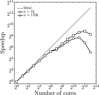
Strong scaling of the MRWT has been evaluated at both early and late times in the simulation of damage nucleation and propagation from Section 5. The time required to complete an embedded $\mathcal{O}(\Delta t^{4})$ and $\mathcal{O}(\Delta t^{5})$ explicit Runge-Kutta integration step (i.e., $n\rightarrow n+1$ ) was measured using Indiana University’s BigRed200, an HPE Cray EX supercomputer where each node is equipped with $256$ GB of memory and two $64$ -core AMD EPYC $7742$ processors [127]. Results bind one MPI process to each socket and continue to use OpenMP within each process. Simultaneous multithreading is not evaluated. The associated speedup is defined with respect to the run-time using only a single core. As shown in Fig. 15, the early time-step (i.e., $n=1,000$ time-steps, $t\approx 0.03\ \mu$ s, and $\mathcal{O}(100$ k) points) strong scales from $225$ s to $1.03$ s per step at $2,048$ cores, at which point communication dominates. The later time-step (i.e., $n=170,000$ time-steps, $t\approx 1.75\ \mu$ s, and $\mathcal{O}(840$ k) points) scales from $2,542$ s to $5.4$ s per step at $4,096$ cores.

Appendix C Taylor-Sedov blast wave

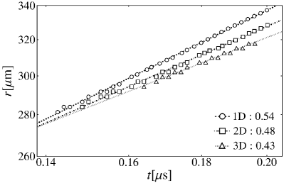
Details of the Taylor-Sedov problem can be found in previous publications [106, 115]. In summary, the Navier-Stokes equations are solved with Fourier’s law of heat conduction and model of a Newtonian fluid as a calorically perfect ideal gas with constant material properties matching those of dry air. The initial condition is a pressure spike in an otherwise undisturbed medium and over time this potential energy is converted into kinetic energy forming a shock wave at a radius $r(t)$ theoretically propagating outward such that [116]

\displaystyle r(t)\propto t^{\frac{2}{2+N}},

(57)

where $N$ is the number of spatial dimensions. In our simulations, the radius of the shock wave is defined as the location of the most extreme pressure gradient. Figure 16 plots the pressure field from the $3$ D simulation using MRWT along with the radius calculations from $1$ D, $2$ D, and $3$ D (see Eq. 57). The slopes match well the theoretical predictions indicating that our wavelet method provides accurate solutions to systems of nonlinear PDEs in multiple dimensions. Note that Figure 16(a) was obtained with $p=6$ and threshold parameters

\displaystyle\varepsilon_{\rho}

\displaystyle=10^{-2}\ \|\ \rho\ \|_{\infty},

\displaystyle\varepsilon_{v_{i}}

\displaystyle=10^{-2}\ \|\ v_{i}\ \|_{\infty},

\displaystyle\varepsilon_{e}

\displaystyle=10^{-2}\ \|\ e\ \|_{\infty},

(58)

where $\rho$ is the density, $v_{i}$ is the $i^{\mathrm{th}}$ component of the velocity, and $e$ is the specific internal energy.

References

Irwin [1957] G. R. Irwin, Analysis of stresses and strains near the end of a crack traversing a plate, Journal of Applied Mechanics 24 (1957) 361–364.
Dugdale [1960] D. S. Dugdale, Yielding of steel sheets containing slits, Journal of the Mechanics and Physics of Solids 8 (1960) 100–104.
Willis [1967] J. R. Willis, A comparison of the fracture criteria of Griffith and Barenblatt, Journal of the Mechanics and Physics of Solids 15 (1967) 151–162.
Spanoudakis and Young [1984] J. Spanoudakis, R. J. Young, Crack propagation in a glass particle-filled epoxy resin part 1. effect of particle volume fraction and size, Journal of Materials Science 19 (1984) 473–486.
Bažant [1986] Z. P. Bažant, Mechanics of distributed cracking, Applied Mechanics Reviews 39 (1986) 675–705.
Ju [1989] J. W. Ju, Energy-based coupled elastoplastic damage models at finite strains, Journal of Engineering Mechanics 115 (1989) 2507–2525.
Needleman [1990] A. Needleman, An analysis of tensile decohesion along an interface, Journal of the Mechanics and Physics of Solids 38 (1990) 289–324.
Fish and Yu [2001] J. Fish, Q. Yu, Multiscale damage modelling for composite materials: Theory and computational framework, International Journal for Numerical Methods in Engineering 52 (2001) 161–191.
Bažant and Jirásek [2002] Z. P. Bažant, M. Jirásek, Nonlocal integral formulations of plasticity and damage: survey of progress, Journal of Engineering Mechanics 128 (2002) 1119–1149.
Buehler et al. [2003] M. J. Buehler, F. F. Abraham, H. Gao, Hyperelasticity governs dynamic fracture at a critical length scale, Nature 426 (2003) 141–146.
Voyiadjis et al. [2004] G. Z. Voyiadjis, R. K. Abu Al-Rub, A. N. Palazotto, Thermodynamic framework for coupling of non-local viscoplasticity and non-local anisotropic viscodamage for dynamic localization problems using gradient theory, International Journal of Plasticity 20 (2004) 981–1038.
Kitey and Tippur [2005] R. Kitey, H. V. Tippur, Role of particle size and filler-matrix adhesion on dynamic fracture of glass-filled epoxy part I. Macromeasurements, Acta Materialia 53 (2005) 1153–1165.
Park et al. [2009] K. Park, G. H. Paulino, J. R. Roesler, A unified potential-based cohesive model of mixed-mode fracture, Journal of the Mechanics and Physics of Solids 57 (2009) 891–908.
Huynh and Belytschko [2009] D. B. P. Huynh, T. Belytschko, The extended finite element method for fracture in composite materials, International Journal for Numerical Methods in Engineering 77 (2009) 214–239.
Kim et al. [2010] D. J. Kim, J. P. Pereira, C. A. Duarte, Analysis of three-dimensional fracture mechanics problems: A two-scale approach using coarse-generalized FEM meshes, International Journal for Numerical Methods in Engineering 81 (2010) 335–365.
Hankinson [1921] R. Hankinson, Investigation of Crushing Strength of Spruce at Varying Angles of Grain, Technical Report, Air Service Information Circular, 1921.
Hill [1948] R. Hill, A theory of the yielding and plastic flow of anisotropic metals, Proceedings of the Royal Society of London 193 (1948) 281–297.
Drucker and Prager [1952] D. C. Drucker, W. Prager, Soil mechanics and plastic analysis or limit design, Quarterly of Applied Mathematics 10 (1952) 157–165.
Tsai and Wu [1971] S. W. Tsai, E. M. Wu, A general theory of strength for anisotropic materials, Journal of Composite Materials 5 (1971) 58–80.
Hoek and Brown [1980] E. Hoek, E. Brown, Empirical strength criterion for rock masses, Journal of the Geotechnical Engineering Division 106 (1980) 1013–1035.
Johnson and Holmquist [1994] G. R. Johnson, T. J. Holmquist, An improved computational constitutive model for brittle materials, in: AIP Conference Proceedings, 1994, pp. 981–984. doi:10.1063/1.46199.
Staat [2021] M. Staat, An extension strain type Mohr–Coulomb criterion, Rock Mechanics and Rock Engineering 54 (2021) 6207–6233.
Griffith [1921] A. A. Griffith, The phenomena of rupture and flow in solids, Philosophical Transactions of the Royal Society of London 221 (1921) 163–198.
Barenblatt [1961] G. I. Barenblatt, The mathematical theory of equilibrium cracks formed in brittle fracture, Zhurnal Prikladnoy Mekhaniki i Tekhnicheskoy Fiziki 4 (1961) 3–56.
Freund [1990] L. B. Freund, Dynamic Fracture Mechanics, Cambridge University Press, Cambridge, 1990. doi:10.1017/CBO9780511546761.
Krajcinovic [1995] D. Krajcinovic, Continuum damage mechanics: when and how?, International Journal of Damage Mechanics 4 (1995) 217–229.
Lemaitre [1971] J. Lemaitre, Evaluation of dissipation and damage in metals submitted to dynamic loading, in: International Conference on the Mechanical Behavior of Materials, 1971, pp. 1–8.
Leckie and Hayhurst [1974] F. A. Leckie, D. R. Hayhurst, Creep rupture of structures, Proceedings of the Royal Society of London. Series A, Mathematical and Physical Sciences 340 (1974) 323–347.
Lemaitre [1985] J. Lemaitre, A continuous damage mechanics model for ductile fracture, Journal of Engineering Materials and Technology 107 (1985) 83–89.
Dragon and Chihab [1985] A. Dragon, A. Chihab, On finite damage: ductile fracture-damage evolution, Mechanics of Materials 4 (1985) 95–106.
Dragon [1985] A. Dragon, Plasticity and ductile fracture damage: study of void growth in metals, Engineering Fracture Mechanics 21 (1985) 875–885.
Krajcinovic and Fonseka [1981] D. Krajcinovic, G. U. Fonseka, The continuous damage theory of brittle materials, Journal of Applied Mechanics 48 (1981) 809–815.
Krajcinovic [1983] D. Krajcinovic, Constitutive equations for damaging materials, Journal of Applied Mechanics 50 (1983) 355–360.
Marigo [1985] J. J. Marigo, Modelling of brittle and fatigue damage for elastic material by growth of microvoids, Engineering Fracture Mechanics 21 (1985) 861–874.
Lemaitre [1984] J. Lemaitre, How to use damage mechanics, Nuclear Engineering and Design 80 (1984) 233–245.
Kachanov [1980] M. Kachanov, Continuum model of medium with cracks, Journal of the Engineering Mechanics Division 106 (1980) 1039–1051.
Chaboche [1981] J.-L. Chaboche, Continuous damage mechanics – a tool to describe phenomena before crack initiation, Nuclear Engineering and Design 64 (1981) 233–247.
Kamrin et al. [2012] K. Kamrin, C. H. Rycroft, J. C. Nave, Reference map technique for finite-strain elasticity and fluid-solid interaction, Journal of the Mechanics and Physics of Solids 60 (2012) 1952–1969.
Matouš et al. [2008] K. Matouš, M. G. Kulkarni, P. H. Geubelle, Multiscale cohesive failure modeling of heterogeneous adhesives, Journal of the Mechanics and Physics of Solids 56 (2008) 1511–1533.
Kulkarni et al. [2010] M. G. Kulkarni, K. Matouš, P. H. Geubelle, Coupled multi-scale cohesive modeling of failure in heterogeneous adhesives, International Journal for Numerical Methods in Engineering 84 (2010) 916–946.
Mosby and Matouš [2015] M. Mosby, K. Matouš, On mechanics and material length scales of failure in heterogeneous interfaces using a finite strain high performance solver, Modelling and Simulation in Materials Science and Engineering 23 (2015).
Simo and Ju [1987a] J. C. Simo, J. W. Ju, Strain- and stress-based continuum damage models – I. Formulation, Int. J. Solids Structures 23 (1987a) 821–840.
Simo and Ju [1987b] J. C. Simo, J. W. Ju, Strain- and stress-based continuum damage models – II. Computational aspects, Int. J. Solids Structures 23 (1987b) 841–869.
Xue et al. [2010] Z. Xue, M. G. Pontin, F. W. Zok, J. W. Hutchinson, Calibration procedures for a computational model of ductile fracture, Engineering Fracture Mechanics 77 (2010) 492–509.
Volokh [2012] K. Y. Volokh, Characteristic length of damage localization in steel, Engineering Fracture Mechanics 94 (2012) 85–86.
Volokh [2013] K. Y. Volokh, Characteristic length of damage localization in concrete, Mechanics Research Communications 51 (2013) 29–31.
Volokh [2011] K. Y. Volokh, Characteristic length of damage localization in rubber, International Journal of Fracture 168 (2011) 113–116.
Krajcinovic and Fanella [1986] D. Krajcinovic, D. Fanella, A micromechanical damage model for concrete, Engineering Fracture Mechanics 25 (1986) 585–596.
Pearson and Yee [1991] R. A. Pearson, A. F. Yee, Influence of particle size and particle size distribution on toughening mechanisms in rubber-modified epoxies, Journal of Materials Science 26 (1991) 3828–3844.
Dekkers and Heikens [1983] M. E. J. Dekkers, D. Heikens, The effect of interfacial adhesion on the tensile behavior of polystyrene-glass-bead composites, Journal of Applied Polymer Science 28 (1983) 3809–3815.
Huang et al. [2004] L. Huang, Q. Yuan, W. Jiang, L. An, S. Jiang, R. K. Li, Mechanical and thermal properties of glass bead-filled nylon-6, Journal of Applied Polymer Science 94 (2004) 1885–1890.
Kinlock and Hunston [1987] A. J. Kinlock, D. L. Hunston, Effect of volume fraction of dispersed rubbery phase on the toughness of rubber-toughened epoxy polymers, Journal of Materials Science Letters 6 (1987) 131–139.
Radford [1971] K. C. Radford, The mechanical properties of an epoxy resin with a second phase dispersion, Journal of Materials Science 6 (1971) 1286–1291.
Nakamura et al. [1992] Y. Nakamura, M. Yamaguchi, Masayoshi Okubo, T. Matsumoto, Effects of particle size on mechanical and impact properties of epoxy resin filled with spherical silica, Journal of Applied Polymer Science 45 (1992) 1281–1289.
Singh et al. [2002] R. P. Singh, M. Zhang, D. Chan, Toughening of a brittle thermosetting polymer: Effects of reinforcement particle size and volume fraction, Journal of Materials Science 37 (2002) 781–788.
Aragón et al. [2013] A. M. Aragón, S. Soghrati, P. H. Geubelle, Effect of in-plane deformation on the cohesive failure of heterogeneous adhesives, Journal of the Mechanics and Physics of Solids 61 (2013) 1600–1611.
Ha and Bobaru [2011] Y. D. Ha, F. Bobaru, Characteristics of dynamic brittle fracture captured with peridynamics, Engineering Fracture Mechanics 78 (2011) 1156–1168.
Ma et al. [2010] G. W. Ma, X. J. Wang, Q. M. Li, Modeling strain rate effect of heterogeneous materials using SPH method, Rock Mechanics and Rock Engineering 43 (2010) 763–776.
Pedersen et al. [2008] R. R. Pedersen, A. Simone, L. J. Sluys, An analysis of dynamic fracture in concrete with a continuum visco-elastic visco-plastic damage model, Engineering Fracture Mechanics 75 (2008) 3782–3805.
Zhou and Molinari [2004] F. Zhou, J. F. Molinari, Dynamic crack propagation with cohesive elements: A methodology to address mesh dependency, International Journal for Numerical Methods in Engineering 59 (2004) 1–24.
Belytschko et al. [2003] T. Belytschko, H. Chen, J. Xu, G. Zi, Dynamic crack propagation based on loss of hyperbolicity and a new discontinuous enrichment, International Journal for Numerical Methods in Engineering 58 (2003) 1873–1905.
Matouš [2003] K. Matouš, Damage evolution in particulate composite materials, International Journal of Solids and Structures 40 (2003) 1489–1503.
Lee et al. [2021] S. Lee, K. Ramos, K. Matouš, Numerical study of damage in particulate composites during high-strain rate loading using novel damage model, Mechanics of Materials 160 (2021).
Kulkarni et al. [2009] M. G. Kulkarni, P. H. Geubelle, K. Matouš, Multi-scale modeling of heterogeneous adhesives: Effect of particle decohesion, Mechanics of Materials 41 (2009) 573–583.
Abedi et al. [2010] R. Abedi, M. A. Hawker, R. B. Haber, K. Matouš, An adaptive spacetime discontinuous Galerkin method for cohesive models of elastodynamic fracture, International Journal for Numerical Methods in Engineering 81 (2010) 1207–1241.
Berger and Oliger [1984] M. J. Berger, J. Oliger, Adaptive mesh refinement for hyperbolic partial differential equations, Journal of Computational Physics 53 (1984) 484–512.
Fatkullin and Hesthaven [2001] I. Fatkullin, J. S. Hesthaven, Adaptive high-order finite-difference method for nonlinear wave problems, Journal of Scientific Computing 16 (2001) 47–67.
Brandt [1977] A. Brandt, Multi-level adaptive solutions to boundary-value problems, Mathematics of Computation 31 (1977) 333–390.
Hackbusch [1978] W. Hackbusch, On the multi-grid method applied to difference equations, Computing 20 (1978) 291–306.
Yushu and Matouš [2020] D. Yushu, K. Matouš, The image-based multiscale multigrid solver, preconditioner, and reduced order model, Journal of Computational Physics 406 (2020).
Benek et al. [1986] J. A. Benek, J. L. Steger, F. C. Dougherty, P. G. Buning, Chimera: A Grid-Embedding Technique, Technical Report, AEDC-TR-85-64, 1986.
Dong and Karniadakis [2003] S. S. Dong, G. E. Karniadakis, P-refinement and P-threads, Computer Methods in Applied Mechanics and Engineering 192 (2003) 2191–2201.
Gui and Babuška [1986a] W. Gui, I. Babuška, The h, p and h-p versions of the finite element method in 1 dimension part I. the error analysis of the p-version, Numerische Mathematik 49 (1986a) 577–612.
Gui and Babuška [1986b] W. Gui, I. Babuška, The h, p and h-p versions of the finite element method in 1 dimension part II. the error analysis of the h-and h-p versions, Numerische Mathematik 49 (1986b) 613–657.
Rajagopal and Sivakumar [2007] A. Rajagopal, S. M. Sivakumar, A combined r-h adaptive strategy based on material forces and error assessment for plane problems and bimaterial interfaces, Computational Mechanics 41 (2007) 49–72.
Jawerth and Sweldens [1994] B. Jawerth, W. Sweldens, An overview of wavlet based multiresolution analyses, SIAM Review 36 (1994) 377–412.
Schneider and Vasilyev [2010] K. Schneider, O. V. Vasilyev, Wavelet methods in computational fluid dynamics, Annual Review of Fluid Mechanics 42 (2010) 473–503.
Liandrat and Tchamitchian [1990] J. Liandrat, P. Tchamitchian, Resolution of the 1D Regularized Burgers Equation Using a Spatial Wavelet Approximation, Technical Report, ICASE 90-83, 1990.
Beylkin and Keiser [1997] G. Beylkin, J. M. Keiser, On the adaptive numerical solution of nonlinear partial differential equations in wavelet bases, Journal of Computational Physics 132 (1997) 233–259.
Bertoluzza [1996] S. Bertoluzza, Adaptive wavelet collocation method for the solution of Burgers equation, Transport Theory and Statistical Physics 25 (1996) 339–352.
Ueno et al. [2003] T. Ueno, T. Ide, M. Okada, A wavelet collocation method for evolution equations with energy conservation property, Bulletin des Sciences Mathematiques 127 (2003) 569–583.
Quian and Weiss [1993] S. Quian, J. Weiss, Wavelets and the numerical solution of partial differential equations, Journal of Computational Physics 106 (1993) 155–175.
Kong et al. [2016] F. Kong, I. A. Kougioumtzoglou, P. D. Spanos, S. Li, Nonlinear systemresponse evolutionary power spectral density determination via a harmonicwavelets based galerkin technique, International Journal for Multiscale Computational Engineering 14 (2016) 255–272.
van Tuijl et al. [2019] R. van Tuijl, C. Harnish, K. Matouš, J. Remmers, M. Geers, Wavelet based reduced order models for microstructural analyses, Computational Mechanics 63 (2019).
Paolucci et al. [2014a] S. Paolucci, Z. J. Zikoski, D. Wirasaet, WAMR: An adaptive wavelet method for the simulation of compressible reacting flow part I. accuracy and efficiency of algorithm, Journal of Computational Physics 272 (2014a) 814–841.
Paolucci et al. [2014b] S. Paolucci, Z. J. Zikoski, T. Grenga, WAMR: An adaptive wavelet method for the simulation of compressible reacting flow part II. the parallel algorithm, Journal of Computational Physics 272 (2014b) 842–864.
Nejadmalayeri et al. [2015] A. Nejadmalayeri, A. Vezolainen, E. Brown-Dymkoski, O. V. Vasilyev, Parallel adaptive wavelet collocation method for PDEs, Journal of Computational Physics 298 (2015) 237–253.
Dubos and Kevlahan [2013] T. Dubos, N. K. Kevlahan, A conservative adaptive wavelet method for the shallow-water equations on staggered grids, Quarterly Journal of the Royal Meteorological Society 139 (2013) 1997–2020.
Sakurai et al. [2017] T. Sakurai, K. Yoshimatsu, K. Schneider, M. Farge, K. Morishita, T. Ishihara, Coherent structure extraction in turbulent channel flow using boundary adapted wavelets, Journal of Turbulence 18 (2017) 352–372.
Fröhlich and Schneider [1994] J. Fröhlich, K. Schneider, An Adaptive Wavelet Galerkin Algorithm for One-Dimensional and 2-Dimensional Flame Computations, European Journal of Mechanics B-Fluids 13 (1994) 439–471.
Goedecker [2009] S. Goedecker, Wavelets and their application for the solution of partial differential equations in physics, Technical Report, Max-Planck Institute for Solid State Research, 2009.
Iqbal and Jeoti [2014] A. Iqbal, V. Jeoti, An Improved Split-Step Wavelet Transform Method for Anomalous Radio Wave Propagation Modeling, Radioengineering 23 (2014) 987–996.
Le and Caracoglia [2015] T. H. Le, L. Caracoglia, Reduced-order wavelet-Galerkin solution for the coupled, nonlinear stochastic response of slender buildings in transient winds, Journal of Sound and Vibration 344 (2015) 179–208.
Lin and Zhou [2001] E. B. Lin, X. Zhou, Connection coefficients on an interval and wavelet solutions of Burgers equation, Journal of Computational and Applied Mathematics 135 (2001) 63–78.
Holmström [1999] M. Holmström, Solving hyperbolic PDEs using interpolating wavelets, SIAM Journal on Scientific Computing 21 (1999) 405–420.
Daubechies [1992] I. Daubechies, Ten Lectures on Wavelets, SIAM, 1992. doi:10.1137/1.9781611970104.
Cohen et al. [2000] A. Cohen, W. Dahmen, R. Devore, Multiscale decompositions on bounded domains, Transactions of the American Mathematical Society 352 (2000) 3651–3685.
Bacry et al. [1992] E. Bacry, S. Mallat, G. Papanicolaou, A Wavelet Based Space-Time Adaptive Numerical Method for Partial Differential Equations, Mathematical Modelling and Numerical Analysis 26 (1992) 793–834.
De Villiers et al. [2004] J. M. De Villiers, K. M. Goosen, B. M. Herbst, Dubuc-Deslauriers subdivision for finite sequences and interpolation wavelets on an interval, SIAM Journal on Mathematical Analysis 35 (2004) 423–452.
Beylkin [1992] G. Beylkin, On the representation of operators in bases of compactly supported wavelets, SIAM Journal on Numerical Analysis 6 (1992) 1716–1740.
Sweldens [1998] W. Sweldens, The lifting scheme: a construction of second generation wavelets, SIAM Journal on Mathematical Analysis 29 (1998) 511–546.
Burgos et al. [2013] R. B. Burgos, M. A. Cetale Santos, R. R. E. Silva, Deslauriers-Dubuc interpolating wavelet beam finite element, Finite Elements in Analysis and Design 75 (2013) 71–77.
Fujii and Hoefer [2003] M. Fujii, W. J. Hoefer, Interpolating wavelet collocation method of time dependent Maxwell’s equations: Characterization of electrically large optical waveguide discontinuities, Journal of Computational Physics 186 (2003) 666–689.
Donoho [1992] D. L. Donoho, Interpolating Wavelet Transforms, Technical Report, Stanford University, 1992.
Harnish et al. [2018] C. Harnish, K. Matouš, D. Livescu, Adaptive wavelet algorithm for solving nonlinear initial–boundary value problems with error control, International Journal for Multiscale Computational Engineering 16 (2018).
Harnish et al. [2021] C. Harnish, L. Dalessandro, K. Matouš, D. Livescu, A multiresolution adaptive wavelet method for nonlinear partial differential equations, International Journal for Multiscale Computational Engineering 19 (2021) 29–37.
Jameson [1993] L. Jameson, On the Daubechies-based wavelet differentiation matrix, Technical Report, ICASE 93-95, 1993.
Dahmen et al. [1999] W. Dahmen, A. Kunoth, K. Urban, Biorthogonal spline wavelets on the interval - stability and moment conditions, Applied and Computational Harmonic Analysis 6 (1999) 132–196.
Farge [1992] M. Farge, Wavelet transforms and their applications to turbulence, Annual Review of Fluid Mechanics 24 (1992) 395–457.
Rioul [1992] O. Rioul, Simple regularity criteria for subdivision schemes, SIAM Journal on Mathematical Analysis 23 (1992) 1544–1576.
Fehlberg [1970] E. Fehlberg, Classical fourth- and lower order Runge-Kutta formulas with stepsize control and their application to heat transfer problems, Computing 6 (1970) 61–71.
Domingues et al. [2009] M. O. Domingues, S. M. Gomes, O. Roussel, K. Schneider, Space-time adaptive multiresolution methods for hyperbolic conservation laws: Applications to compressible Euler equations, Applied Numerical Mathematics 59 (2009) 2303–2321.
Pathria [1997] D. Pathria, The correct formulation of intermediate boundary conditions for Runge-Kutta time integration of initial boundary value problems, SIAM Journal on Scientific Computing 18 (1997) 1255–1266.
Hesthaven and Gottlieb [1996] J. S. Hesthaven, D. Gottlieb, A stable penalty method for the compressible Navier-Stokes equations: I. Open boundary conditions, SIAM Journal on Scientific Computing 17 (1996) 579–612.
Schlick et al. [2021] T. Schlick, S. Portillo-Ledesma, M. Blaszczyk, L. Dalessandro, S. Ghosh, K. Hackl, C. Harnish, S. Kotha, D. Livescu, A. Masud, K. Matouš, A. Moyeda, C. Oskay, J. Fish, A multiscale vision – illustrative applications from biology to engineering, International Journal for Multiscale Computational Engineering 19 (2021) 39–73.
Sedov [1946] L. I. Sedov, Propagation of strong shock waves, Journal of Applied Mathematics and Mechanics 10 (1946) 241–250.
Ju J [1989] Ju J, On energy-based coupled elastoplastic damage theories: constitutive modeling and compuational aspects, International Journal of Solids and Structures 25 (1989) 803–833.
Ahmed and Khan [2021] A. Ahmed, R. Khan, A phase field model for damage in asphalt concrete, International Journal of Pavement Engineering (2021).
Christman [1972] D. R. Christman, Dynamic properties of poly (methylmethacrylate) (PMMA) (Plexiglas), Technical Report, GM Technical Center, Warren, Michigan, 1972.
Cheng et al. [1990] W. M. Cheng, G. A. Miller, J. A. Manson, R. W. Hertzberg, L. H. Sperling, Mechanical behaviour of poly(methyl methacrylate) – Part 1 Tensile strength and fracture toughness, Journal of Materials Science 25 (1990) 1917–1923.
Pluvinage and Capelle [2014] G. Pluvinage, J. Capelle, On characteristic lengths used in notch fracture mechanics, International Journal of Fracture 187 (2014) 187–197.
Wu et al. [2004] H. Wu, G. Ma, Y. Xia, Experimental study of tensile properties of PMMA at intermediate strain rate, Materials Letters 58 (2004) 3681–3685.
Chen et al. [2002] W. Chen, F. Lu, M. Cheng, Tension and compression tests of two polymers under quasi-static and dynamic loading, Polymer Testing 21 (2002) 113–121.
Miller et al. [1999] O. Miller, L. B. Freund, A. Needleman, Energy dissipation in dynamic fracture of brittle materials, Modelling and Simulation in Materials Science and Engineering 7 (1999) 573–586.
Zhang et al. [2007] Z. J. Zhang, G. H. Paulino, W. Celes, Extrinsic cohesive modelling of dynamic fracture and microbranching instability in brittle materials, International Journal for Numerical Methods in Engineering 72 (2007) 893–923.
Xu and Needleman [1994] X.-P. Xu, A. Needleman, Numerical simulations of fast crack growth in brittle solids, Journal of the Mechanics and Physics of Solids 42 (1994) 1397–1434.
Stewart et al. [2017] C. Stewart, V. Welch, B. Plale, G. Fox, M. Pierce, T. Sterling, Indiana University Pervasive Technology Institute, 2017. URL: https://pti.iu.edu/. doi:10.5967/K8G44NGB.


(a)	(b)

(c)	(d)


(a)	(b)

(c)	(d)


(a)	(b)

(c)	(d)