An Adaptive State Aggregation Algorithm for Markov Decision Processes
Abstract
Value iteration is a well-known method of solving Markov Decision Processes (MDPs) that is simple to implement and boasts strong theoretical convergence guarantees. However, the computational cost of value iteration quickly becomes infeasible as the size of the state space increases. Various methods have been proposed to overcome this issue for value iteration in large state and action space MDPs, often at the price, however, of generalizability and algorithmic simplicity. In this paper, we propose an intuitive algorithm for solving MDPs that reduces the cost of value iteration updates by dynamically grouping together states with similar cost-to-go values. We also prove that our algorithm converges almost surely to within of the true optimal value in the norm, where is the discount factor and aggregated states differ by at most . Numerical experiments on a variety of simulated environments confirm the robustness of our algorithm and its ability to solve MDPs with much cheaper updates especially as the scale of the MDP problem increases.
1 Introduction
State aggregation is a long-standard approach to solving large-scale Markov decision processes (MDPs). The main idea of state aggregation is to define the similarity between states, and work with a system of reduced complexity size by grouping similar states into aggregate, or “mega-”, states. Although there has been a variety of results on the performance of the policy using state aggregation li2006 ; van2006 ; abel2016 , a common assumption is that states are aggregated according to the similarity of their optimal cost-to-go values. Such a scheme, which we term pre-specified aggregation, is generally infeasible unless the MDP is already solved. To address the difficulties inherent in pre-specified aggregation, algorithms that learn how to effectively aggregate states have been proposed ortner2013 ; duan2018 ; sinclair2019 .
This paper aims to provide new insights into adaptive online learning of the correct state aggregates. We propose a simple and efficient state aggregation algorithm for calculating the optimal value and policy of an infinite-horizon discounted MDP that can be applied in planning problems baras2000 and generative MDP problems sidford2018near . The algorithm alternates between two distinct phases. During the first phase (“global updates”), the algorithm updates the cost-to-go values as in the standard value iteration, trading off some efficiency to more accurately guide the cost-to-go values in the right direction; in the second phase (“aggregate updates”), the algorithm groups together states with similar cost-to-go values based on the last sequence of global updates then efficiently updates the states in each mega-state in tandem as it optimizes over the reduced space of aggregate states.
The algorithm is simple: the inputs needed for state aggregation are the current cost-to-go values and the parameter , which bounds the difference between (current) cost to go values of states within a given mega-state. Compared to prior works on state aggregation that use information on the state-action value (-value) sinclair2019 , transition density ortner2013 , and methods such as upper confidence intervals, our method does not require strong assumptions or extra information, and only performs updates in a manner similar to standard value iteration.
Our contribution is a feasible online algorithm for learning aggregate states and cost-to-go values that requires no extra information beyond that required for standard value iteration. We showcase in our experimental results that our method provides significantly faster convergence than standard value iteration especially for problems with larger state and action spaces. We also provide theoretical guarantees for the convergence, accuracy, and convergence rate of our algorithm.
The simplicity and robustness of our novel state aggregation algorithm demonstrates its utility and general applicability in comparison to existing approaches for solving large MDPs.
1.1 Related literature
When a pre-spcified aggregation is given, tsitsiklis1996 ; van2006 give performance bounds on the aggregated system and propose variants of value iteration. There are also a variety of ways to perform state aggregation based on different criteria. ferns2012 ; dean1997 analyze partitioning the state space by grouping states whose transition model and reward function are close. mccallum1997 proposes aggregate states that have the same optimal action and similar -values for these actions. jong2005 develops aggregation techniques such that states are aggregated if they have the same optimal action. We refer the readers to li2006 ; abel2016 ; abel2020 for a more comprehensive survey on this topic.
On the dynamical learning side, our adaptive state-aggregated value iteration algorithm is also related to the aggregation-disaggregation method used to accelerate the convergence of value iterations (bertsekas1988 ; schweitzer1985 ; mendelssohn1982 ; bertsekas2018 ) in policy evaluation, i.e., to evaluate the value function of a policy. Among those works, that of bertsekas1988 is closest to our approach. Assuming the underlying Markov processes to be ergodic, the authors propose to group states based on Bellman residuals in between runs of value iteration. They also allow states to be aggregated or disaggregated at every abstraction step. However, the value iteration step in our setting is different from the value iteration in bertsekas1988 for the reason that value iteration in policy evaluation will not involve the Bellman operator. Aside from state aggregation, a variety of other methods have been studied to accelerate value iteration. herzberg1994 proposes iterative algorithms based on a one-step look-ahead approach. shlakhter2010 combines the so called “projective operator” with value iteration and achieve better efficiency. anderson1965 ; fang2009 ; zhang2020 analyze the Anderson mixing approach to speed up the convergence of fixed-point problems.
Dynamic learning of the aggregate states has also been studied more generally in MDP and reinforcement learning (RL) settings. hostetler2014 proposes a class of -value–based state aggregations and applies them to Monte Carlo tree search. slivkins2011 uses data-driven discretization to adaptively discretize state and action space in a contextual bandit setting. ortner2013 develops an algorithm for learning state aggregation in an online setting by leveraging confidence intervals. sinclair2019 designs a -learning algorithm based on data-driven adaptive discretization of the state-action space. For more state abstraction techniques see baras2000 ; dean1997 ; jiang2014 ; abel2019 .
2 Preliminaries
2.1 Markov decision process
We consider an infinite-horizon Markov Decision Process , consisting of: a finite state space ; a finite action space ; the probability transition model , where denotes the probability of transitioning to state conditioned on the state-action pair ; the immediate cost function , which denotes the immediate cost—or reward—obtained from a particular state-action pair; the discount factor ; and the initial distribution over states in , which we denote by .
A policy specifies the agent’s action based on the current state, either deterministically or stochastically. A policy induces a distribution over the trajectories , where , and and for .
A value function assigns a value to each state; as , can also be represented by a finite-length vector . (In this paper, we view all vector as vector functions mapping from the index to the corresponding entry.) Moreover, each policy is associated with a value function , which is defined to be the discounted sum of future rewards starting at and with policy :
As noted above, we represent both the value function corresponding to the policy and the value vector as .
For each state and action belonging to state , let denote the vector of transition probabilities resulting from taking the action in state . We call a policy greedy with respect to a given value if
We define to be the dynamic programming operator such that where
The optimal value function is the unique solution of the equation . A common approach to find is value iteration, which, given an initial guess , generates a sequence of value functions such that . The sequence converges to as goes to Bel .
2.2 State aggregation
The state space of MDPs can be very large. State aggregation divides the state space into subsets and views each collection of states as a mega-state. Then, the value function generated by the mega-states can be used to approximate the optimal value .
To represent a state aggregation, we define the matrix . We set if state is in the -th mega-state, and let otherwise; i.e., column of indicates whether each state belongs to mega-state . The state-reduction matrix also induces a partition on , i.e., and for . Denote by the cost-to-go value function for the aggregated state, and note that the current value of induces a value function on the original state space, where
3 Algorithm design
In this section, we first introduce a state aggregation algorithm which assumes knowledge of the optimal value function. The algorithm is proposed in tsitsiklis1996 which also provides the corresponding convergence result. Based on existing theory, we design our adaptive algorithm and discuss its convergence properties.
3.1 A pre-speficied aggregation algorithm
Given a pre-specified aggregation, we seek the value function for the aggregated states such that
| (1) |
where and for . Intuitively, Eq. justifies our approach of aggregating states that have similar optimal cost-to-go values. We then state the algorithm that will converge to the correct cost-to-go values while satisfying Eq. .
Algorithm 1 takes a similar form in Stochastic Approximation robbins1951 ; wasan2004 , and will converge almost surely to a unique cost-to-go value. Here is the step size of the learning algorithm; by taking, e.g., , we recover the formula of value iteration. The following convergence result is proved in tsitsiklis1996 .
Proposition 1 (Theorem 1, tsitsiklis1996 ).
When and , in Line 6 of Algorithm 1 will converge almost surely to entry-wise, where is the solution of
| (2) |
Define to be the greedy policy with respect to . Then, we have, morevoer, that
| (3) | ||||
where is the value function associated with policy .
Proposition 1 states that if we are able to partition the state space such that the maximum difference of the optimal value function within each mega-state is small, the value function produced by Algorithm 1 can approximate the optimal value up to , and the policy associated with the approximated value function will also be close to the optimal policy.
3.2 Value iteration with state aggregation
In order to generate an efficient approximation, Proposition 1 requires a pre-specified aggregation scheme such that is small for every to guarantee the appropriate level of convergence for Algorithm 1. Without knowing , is it still possible to control the approximation error? In this section we answer in the affirmative by introducing an adaptive state aggregation scheme that learns the correct state aggregations online as it learns the true cost-to-go values.
Given the current cost-to-go value vector , let , let . Group the cost-to-go values among disjoint subintervals of the form . Next, let , and let to be the -th mega-state, which contains all the states whose current estimated cost-to-go value falls in the interval . Grouping the states in this way reduces the state size from states to at most mega-states. See Algorithm 2 for further details.
Without the knowledge of in advance, one must periodically perform value iteration on to learn the correct aggregation to help with adapting the aggregation scheme. As a result, our algorithm alternates between two phases: in the global update phase the algorithm performs value iteration on ; in the aggregated update phase, the algorithm starts to group together states with similar cost-to-go values based on the result of the last global update, and then performs aggregated updates as in Algorithm 1.
We denote by the intervals of iterations in which the algorithm performs state-aggregated updates, and we denote by the intervals of iterations in which the algorithm performs global update. As a consequence, for any and ; likewise, for any and .
We then present our adaptive algorithm. For a pre-speficied number of iterations , the time horizon is divided into intervals of the form . Every time the algorithm exits an interval of global updates , it runs Algorithm 2 based on the current cost-to-go value and the parameter , using the output of Algorithm 2 for the current state aggregation and cost-to-go values for . Similarly, every time the algorithm exits an interval of state-aggregated updates , it sets , where is the current cost-to-go value for the aggregated space, as the initial cost-to-go value for the subsequent interval of global iterations.
| (4) |
3.3 Convergence
From Proposition 1, if we fix the state-aggregation parameter , even with perfect information, state aggregated value iteration will generate an approximation of the cost-to-go values with error bounded by . This bound is sharp, as shown in tsitsiklis1996 . Such error is negligible in the early phase of the algorithm, but the error would accumulate in the later phase of the algorithm and prevent the algorithm from converging to the optimal value. As a result, it is not desirable for .111 By setting adaptively, one might achieve better complexity and error bound by setting ; however, adaptively choosing lies beyond the scope of this work.
We state asymptotic convergence results for Algorithm 3; proofs can be found in the supplementary materials. For the remainder of the paper, by a slight abuse of notation, we denote by the current cost-to-go value at iteration . More specifically, if the current algorithm is in phase , is the updated cost-to-go value for global value iteration. If the algorithm is in phase , represents .
Theorem 1.
If , and , we have
Notice that the result of Theorem 1 is consistent with Proposition 1: due to state aggregation we suffer from the same for the error bound. However, our algorithm maintains the same order of error bound without knowing the optimal value function .
We also identify the existence of “stable field” for our algorithm, and we prove that under some specific choice of the learning rate , with probability one the value function will stay within the stable field.
Proposition 2.
If for all , we have that after iterations, with probability one the estimated approximation satisfies
for any choice of initialization .
Proposition 3.
For , if , after iterations, with probability one the estimated approximation satisfies
for any choice of initialization .
Such results provide guidance for choice of parameters. Indeed, the experimental results are consistent with the theory presented above.


4 Experiments
To test the theory developed in Sections 3, we perform a number of numerical experiments.222All experiments were performed in parallel using forty Xeon E5-2698 v3 @ 2.30GHz CPUs. Total compute time was approximately 60 hours. Code and replication materials are available in the Supplementary Materials. We test our methods on a variety of MDPs of different sizes and complexity. Our results show that state aggregation can achieve faster convergence than standard value iteration; that state aggregation scales appropriately as the size and dimensionality of the underlying MDP increases; and that state aggregation is reasonably robust to measurement error (simulated by adding noise to the action costs) and varying levels of stochasticity in the transition matrix.


4.1 MDP problems
We consider two problems in testing our algorithm. The first, which we term the “standard maze problem” consists of a grid of positions. Each position is connected to one or more adjacent positions. Moving from position to position incurs a constant cost, except for moving to the terminal state of the maze (the position ) which incurs a constant reward.333 We rescale action costs in both the standard and terrain mazes to ensure that the maximum cost-to-go is exactly 100. There is a unique path from each position to the terminal state. A two-dimensional standard maze, in which the player can move, depending on their position, up, down left, or right is illustrated in Figure 1(a).
The second problem is the “terrain maze problem.” As in a standard maze, each state in the terrain maze represents a position in a grid. As before, we imagine that the player can move from state to state only by travelling a single unit in any direction. (The player is only constrained from moving out of the grid entirely.) The player receives a reward for reaching the final square of the maze, which again we place at position . However, in contrast to the standard maze game, the player’s movements incur different costs at different positions. In particular, the maze is determined by a “height function” . The cost of movement is set to be the difference in heights between the player’s destination position and their current position, normalized appropriately.
In both problems, we also allow for stochasticity controlled by a parameter which gives the probability that a player moves in their intended direction. For , the MDP is deterministic; otherwise, with probability , the player moves in a different direction chosen uniformly at random.
In both problems, the actions available at any state correspond to a very sparse transition probability vectors, since players are constrained to move along cardinal directions at a rate of a single unit. However, in the standard maze game, the cost-to-go at any position is extremely sensitive to the costs-to-go at states that are very distant. In a standard maze, the initial tile (i.e., position (1, 1)) is often between 25 and 30 units away from the destination tile (i.e., position (10, 10)). In contrast, in the terrain maze game, the cost-to-go is much less sensitive to far away positions, because local immediate costs, dictated by the slopes one must climb or go down to move locally, are more significant.
4.1.1 Benchmarks and parameters
We measure convergence by the -distance (hereafter “error”) between the current cost-to-go vector and the true cost-to-go vector, and we evaluate the speed based on the size of error and the number of updates performed. Notice that for global value iteration, an update for state has the form
and an update for mega-state (represented by ) has the form
Because the transition matrix is not dense in our examples, the computational resources required for global value iteration update and aggregated update are roughly the same. For each iteration, the value iteration will always perform updates, and for Algorithm 3, only updates, one for each mega-state, will be performed if in the aggregation phase.
All experiments are performed with a discount factor . We set and for every , and for learning rate we set . The cost function is normalized such that , and we choose aggregation constant to be (unless otherwise indicated). We set the initial cost vector to be the zero vector .
4.1.2 Results
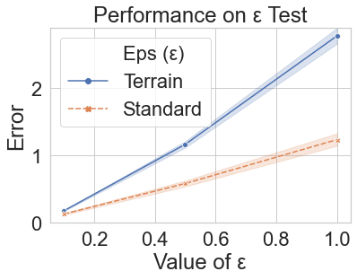
Influence of .
We test the effect of on the error Algorithm 3 produces. We run experiments with aggregation constant , and for standard and terrain mazes. For each , we run 1,000 iterations of Algorithm 3, and each experiment is repeated 20 times; the results, shown in Figure 2(a), indicate that the approximation error scales in proportion to , which is consistent with Proposition 1 and Theorem 1.
Efficiency.
We test the convergence rate of Algorithm 3 against value iteration on standard and terrain mazes, repeating each experiment 20 times. From Figure 2(b) and 2(c), we see that state-aggregated value iteration is very efficient at the beginning phase, converging in fewer updates than value iteration.
| Type | Dims. | Error | 95% CI |
|---|---|---|---|
| Trn. | 4.41 | ||
| Trn. | 4.34 | ||
| Trn. | 4.65 | ||
| Trn. | 4.27 | ||
| Trn. | 4.27 | ||
| Std. | 1.43 | ||
| Std. | 1.39 | ||
| Std. | 1.42 | ||
| Std. | 1.11 | ||
| Std. | 1.40 |
| Type | Dims. | Error | 95% CI |
|---|---|---|---|
| Trn. | 1.91 | ||
| Trn. | 3.02 | ||
| Trn. | 3.59 | ||
| Trn. | 3.85 | ||
| Std. | 1.36 | ||
| Std. | 1.36 | ||
| Std. | 1.23 | ||
| Std. | 1.31 |
| Type | Error | 95% CI | ||
|---|---|---|---|---|
| Terrain | 0.92 | 0.00 | 4.44 | |
| Terrain | 0.92 | 0.01 | 4.41 | |
| Terrain | 0.92 | 0.05 | 4.97 | |
| Terrain | 0.92 | 0.10 | 6.36 | |
| Terrain | 0.95 | 0.00 | 4.43 | |
| Terrain | 0.95 | 0.01 | 4.32 | |
| Terrain | 0.95 | 0.05 | 4.93 | |
| Terrain | 0.95 | 0.10 | 6.39 | |
| Terrain | 0.98 | 0.00 | 4.37 | |
| Terrain | 0.98 | 0.01 | 4.31 | |
| Terrain | 0.98 | 0.05 | 5.01 | |
| Terrain | 0.98 | 0.10 | 6.52 |
| Type | Error | 95% CI | ||
|---|---|---|---|---|
| Standard | 0.92 | 0.00 | 1.39 | |
| Standard | 0.92 | 0.01 | 1.61 | |
| Standard | 0.92 | 0.05 | 2.62 | |
| Standard | 0.92 | 0.10 | 5.56 | |
| Standard | 0.95 | 0.00 | 1.49 | |
| Standard | 0.95 | 0.01 | 1.57 | |
| Standard | 0.95 | 0.05 | 2.86 | |
| Standard | 0.95 | 0.10 | 5.72 | |
| Standard | 0.98 | 0.00 | 1.43 | |
| Standard | 0.98 | 0.01 | 1.88 | |
| Standard | 0.98 | 0.05 | 3.48 | |
| Standard | 0.98 | 0.10 | 5.86 |
Scalibility of state aggregation.
We run state-abstracted value iteration on standard and terrain mazes of size , , , , and for 1000 iterations. We repeat each experiment 20 times, displaying the results in Table 1. Next, we run state-aggregated value iteration on terrain mazes of increasingly large underlying dimension, as shown in the right side of Table 1, likewise for 20 repetitions for each size. The difference with the previous experiment is that not only does the state space increase, the action space also increases exponentially. Our results show that the added complexity of the high-dimensional problems does not appear to substantially affect the convergence of state-aggregated value iteration and our method is able to scale with very large MDP problems.
Robustness.
We examine the robustness of state-aggregated value iteration to two sources of noise. We generate standard and terrain mazes, varying the level of stochasiticity by setting . We also vary the amount of noise in the cost vector by adding a mean 0, standard deviation normal vector to the action costs. The results, shown in Table 2, indicate that state-aggregated value iteration is reasonably robust to stochasiticity and measurement error.
4.2 Continuous Control Problems
We conclude the experiments section by showing the performance of our method on a real-world use case in continuous control. These problems often involve solving complex tasks with high-dimensional sensory input. The idea typically involves teaching an autonomous agent, usually a robot, to successfully complete some task or achieve some goal state. These problems are often very tough as they reside in the continuous state space (and many times action space) domain.
We already showcased the significant reduction in algorithm update costs during learning on grid-world problems in comparison with value iteration. Our goal for this section is to showcase real world examples of how our method may be practically applied in the field of continuous control. This is important not only to emphasize that our idea has a practical use case, but also to further showcase its ability to scale into extremely large (and continuous) dimensional problems.
4.2.1 Environment
We choose to use the common baseline control problem in the "CartPole" system. The CartPole system is a typical physics control problem where a pole is attached to a central joint of a cart, which moves along an endless friction-less track. The system is controlled by applying a force to either move to the right or left with the goal to balance the pole, which starts upright. The system terminates if (1) the pole angle is more than degrees from the vertical axis, or (2) the cart position is more than cm from the center, or (3) the episode length is greater than time-steps.
During each episode, the agent will receive constant reward for each step it takes. The state-space is the continuous position and angle of the pole for the cartpole pendulum system and the action-space involves two actions - applying a force to move the cart left or right. A more in-depth explanation of the problem can be found in DBLP:journals/corr/abs-2006-04938 .
4.2.2 Results
Since the CartPole problem is a multi-dimensional continuous control problem, there is no ground truth -values so we choose to utilize the dense reward nature of this problem and rely on the accumulated reward to quantify algorithm performance as opposed to error. In addition, since value iteration requires discrete states, we discretize all continuous dimensions of the state space into bins and generate policies on the discretized environment. More specifically, we discretize the continuous state space into bins by dividing each dimension of the domain into equidistant intervals.
For our aggregation algorithm, we use following what is commonly used in this problem in past works. We set the initial cost vector to be the zero vector. We fix and set . We note that given the symmetric nature of this continuous control problem, we do not need to alternate between global and aggregate updates. The adaptive aggregation of states already groups states effectively together for strong performance and significant speedups in the number of updates required. We first do a sweep of number of bins to discretize the problem space to determine the number that best maximizes the performance of value iteration in terms of both update number and reward and found this to be around 2000 bins. We then compare the performances of state aggregation and value iteration on this setting in figure 3. To also further showcase the adaptive advantage of our method, we choose a larger bin (10000) number that likely would have been chosen if no bin sweeping had occurred and show that our method acts as an "automatic bin adjuster" and offers the significant speedups without any prior tuning in figure 3. Interestingly in both situations, the experimental results show that the speedup offered by our method seem significant across different bin settings of the CartPole problem. These results may prove to have strong theoretical directions in future works.


5 Discussion
Value iteration is an effective tool for solving Markov decision processes but can quickly become infeasible in problems with large state and action spaces. To address this difficulty, we develop adaptive state-aggregated value iteration, a novel method of solving Markov decision processes by aggregating states with similar cost-to-go values and updating them in tandem. Unlike previous methods of reducing the dimensions of state and action spaces, our method is general and does not require prior knowledge of the true cost-to-go values to form aggregate states. Instead our algorithm learns the cost-to-go values online and uses them to form aggregate states in an adaptive manner. We prove theoretical guarantees for the accuracy, convergence, and convergence rate of our state-aggregated value iteration algorithm, and demonstrate its applicability through a variety of numerical experiments.
State- and action-space reduction techniques are an area of active research. Our contribution in the dynamic state-aggregated value iteration algorithm provides a general framework for approaching large MDPs with strong numerical performances justifying our method. We believe our algorithm can serve as a foundational ground for both future empirical and theoretical work.
We conclude by discussing promising directions for future work on adaptive state aggregation. First, we believe that reducing the number of updates per state by dynamically aggregating states can also be extended more generally in RL settings with model-free methods. Second, our proposed algorithm’s complexity is of the same order as value iteration. Future work may seek to eliminate the dependence on in the error bound. Lastly, by adaptively choosing , it may be possible to achieve better complexity bounds not only for planning problems but also for generative MDP models sidford2018 ; sidford2018near .
References
- [1] D. Abel, D. Arumugam, K. Asadi, Y. Jinnai, M. L. Littman, and L. L. Wong. State abstraction as compression in apprenticeship learning. In Proceedings of the AAAI Conference on Artificial Intelligence, volume 33, pages 3134–3142, 2019.
- [2] D. Abel, D. Hershkowitz, and M. Littman. Near optimal behavior via approximate state abstraction. In International Conference on Machine Learning, pages 2915–2923. PMLR, 2016.
- [3] D. Abel, N. Umbanhowar, K. Khetarpal, D. Arumugam, D. Precup, and M. Littman. Value preserving state-action abstractions. In International Conference on Artificial Intelligence and Statistics, pages 1639–1650. PMLR, 2020.
- [4] D. G. Anderson. Iterative procedures for nonlinear integral equations. Journal of the ACM (JACM), 12(4):547–560, 1965.
- [5] J. Baras and V. Borkar. A learning algorithm for markov decision processes with adaptive state aggregation. In Proceedings of the 39th IEEE Conference on Decision and Control (Cat. No. 00CH37187), volume 4, pages 3351–3356. IEEE, 2000.
- [6] R. Bellman. A markovian decision process. Indiana Univ. Math. J., 6:679–684, 1957.
- [7] D. P. Bertsekas. Feature-based aggregation and deep reinforcement learning: A survey and some new implementations. IEEE/CAA Journal of Automatica Sinica, 6(1):1–31, 2018.
- [8] D. P. Bertsekas, D. A. Castanon, et al. Adaptive aggregation methods for infinite horizon dynamic programming. 1988.
- [9] T. Dean, R. Givan, and S. Leach. Model reduction techniques for computing approximately optimal solutions for markov decision processes. In Proceedings of the Thirteenth Conference on Uncertainty in Artificial Intelligence, UAI’97, page 124–131, San Francisco, CA, USA, 1997. Morgan Kaufmann Publishers Inc.
- [10] Y. Duan, Z. T. Ke, and M. Wang. State aggregation learning from markov transition data. arXiv preprint arXiv:1811.02619, 2018.
- [11] H.-r. Fang and Y. Saad. Two classes of multisecant methods for nonlinear acceleration. Numerical Linear Algebra with Applications, 16(3):197–221, 2009.
- [12] N. Ferns, P. Panangaden, and D. Precup. Metrics for markov decision processes with infinite state spaces. arXiv preprint arXiv:1207.1386, 2012.
- [13] M. Herzberg and U. Yechiali. Accelerating procedures of the value iteration algorithm for discounted markov decision processes, based on a one-step lookahead analysis. Operations Research, 42(5):940–946, 1994.
- [14] J. Hostetler, A. Fern, and T. Dietterich. State aggregation in monte carlo tree search. In Proceedings of the AAAI Conference on Artificial Intelligence, volume 28, 2014.
- [15] N. Jiang, S. Singh, and R. Lewis. Improving uct planning via approximate homomorphisms. In Proceedings of the 2014 international conference on Autonomous agents and multi-agent systems, pages 1289–1296, 2014.
- [16] N. K. Jong and P. Stone. State abstraction discovery from irrelevant state variables. In IJCAI, volume 8, pages 752–757. Citeseer, 2005.
- [17] S. Kumar. Balancing a cartpole system with reinforcement learning - A tutorial. CoRR, abs/2006.04938, 2020.
- [18] L. Li, T. J. Walsh, and M. L. Littman. Towards a unified theory of state abstraction for mdps. ISAIM, 4:5, 2006.
- [19] R. McCallum. Reinforcement learning with selective perception and hidden state. 1997.
- [20] R. Mendelssohn. An iterative aggregation procedure for markov decision processes. Operations Research, 30(1):62–73, 1982.
- [21] R. Ortner. Adaptive aggregation for reinforcement learning in average reward markov decision processes. Annals of Operations Research, 208(1):321–336, 2013.
- [22] H. Robbins and S. Monro. A stochastic approximation method. The annals of mathematical statistics, pages 400–407, 1951.
- [23] P. J. Schweitzer, M. L. Puterman, and K. W. Kindle. Iterative aggregation-disaggregation procedures for discounted semi-markov reward processes. Operations Research, 33(3):589–605, 1985.
- [24] O. Shlakhter, C.-G. Lee, D. Khmelev, and N. Jaber. Acceleration operators in the value iteration algorithms for markov decision processes. Operations research, 58(1):193–202, 2010.
- [25] A. Sidford, M. Wang, X. Wu, L. F. Yang, and Y. Ye. Near-optimal time and sample complexities for solving markov decision processes with a generative model. In Proceedings of the 32nd International Conference on Neural Information Processing Systems, pages 5192–5202, 2018.
- [26] A. Sidford, M. Wang, X. Wu, and Y. Ye. Variance reduced value iteration and faster algorithms for solving markov decision processes. In Proceedings of the Twenty-Ninth Annual ACM-SIAM Symposium on Discrete Algorithms, pages 770–787. SIAM, 2018.
- [27] S. R. Sinclair, S. Banerjee, and C. L. Yu. Adaptive discretization for episodic reinforcement learning in metric spaces. Proceedings of the ACM on Measurement and Analysis of Computing Systems, 3(3):1–44, 2019.
- [28] A. Slivkins. Contextual bandits with similarity information. In Proceedings of the 24th annual Conference On Learning Theory, pages 679–702. JMLR Workshop and Conference Proceedings, 2011.
- [29] J. N. Tsitsiklis and B. Van Roy. Feature-based methods for large scale dynamic programming. Machine Learning, 22(1):59–94, 1996.
- [30] B. Van Roy. Performance loss bounds for approximate value iteration with state aggregation. Mathematics of Operations Research, 31(2):234–244, 2006.
- [31] M. T. Wasan. Stochastic approximation. Number 58. Cambridge University Press, 2004.
- [32] J. Zhang, B. O’Donoghue, and S. Boyd. Globally convergent type-i anderson acceleration for nonsmooth fixed-point iterations. SIAM Journal on Optimization, 30(4):3170–3197, 2020.
Appendix A Appendix
A.1 Preliminaries
Since the number state-action pairs is finite, without loss of generality we can assume that the cost function is bounded by . By a slight abuse of notation, we denote by the current cost-to-go value at iteration generated by Algorithm 3. More specifically, if the current algorithm is in global value iteration phase , is the updated cost-to-go value for global value iteration. If the algorithm is in state aggregation phase , represents . Also, denote by the error between the current estimate and the optimal value function. We first state results on the norm of and .
Lemma 1.
For any we have and .
Lemma 1 states that both of the optimal cost-to-go value and the value obtained by Algorithm 3 is uniformly bounded by entry-wisely at all aggregated and global iterations.
Next, it is well known that can only decrease in the global value iteration phase due to the fact that the Bellman operator is a contraction mapping. However, can potentially grown when we switch into a state aggregation phase. To evaluate the fluctuation of during the state aggregation phase, we firstly notice that the step 4 in Algorithm 2 (which is the initialization step for state aggregation) will generate a tight bound: if we denote to be the initialization result in step 4 Algorithm 2, we will have
| (5) |
The inequality above is tight because by construction there exists a scenario such that and for some .
After the error introduced in the initialization stage of stage aggregation, the value updates process may also accumulate error. Recall that during each state aggregation phase , for we have the following updates for mega-state
Hence by combining Lemma 1, we know that for every SA iteration we have
We then state a general condition that will control the error bound of the state aggregation value update, and we will show that all of our theorem and propositions satisfy such condition.
Condition 1.
There exists such that for any state aggregation phase coming after state aggregation iterations, we have
| (6) |
During state aggregation phase, from we know that the if we switch from to , can increase by , and from Condition 1 we know that after steps of value iteration, can increase by another .
More specifically, after iterations suggested by Condition 1, if we take and , from our discussion above we have
| (7) |
Moreover, the above equation also holds for all , as the Bellman operator is a contraction.
Then, for notational convenience, we re-index the first global iteration phase after SA iterations to be , the following time interval to be . We also denote and ; see Figure 4.
Since , there exists such that for any and we have
| (8) | ||||
where the first inequality comes from the fact that during the global value iteration is performed. The second inequality comes from combining and .
The intuition of is that from to , our approximation will only get better because we are using global value iteration only. From time to , the approximation within the entire SA value iteration phase will stay within the previous error up to another . By balancing those bounds we are able to get a “stable field” for all phases.
We then state the bounds for the error at for
Lemma 2.
For all , we have
| (9) |
From Lemma 2 and , we can generate bounds for all that is large.

A.2 Proof of Theorem 1
Since
there exists such that we have that when , will be bounded from above and will be bounded from below. We denotes those two constants for the bound as and , respectively. Then, since the sequence goes to zero as goes to infinity, there exists a constant such that for we have . Thus, we have
Therefore, we have shown that Condition 1 has been satisfied.
Next, we show that grows nearer to as increases. To see this, by directly applying Lemma 2, we have
and, thus,
Then, in order to prove the final statement of the theorem, we aim to show that for any positive constant , there exists a constant so that for any , the following inequality holds
| (10) |
Since , we can find such that for any , we have
| (11) |
Then, by defining , it suffices to show Eq. (10) for and separately. If for some , from inequality we have
Thus,
where the first line is obtained by the triangle inequality and Eq. (11). If for some , based on the contraction property of Value-Iteration method, we have . Hence, we have shown that Eq. (10) holds for all and any , which is equivalent to
Moreover, if we set and the step size satisfies for all , we have and . Then, we also can obtain Proposition 2 using a similar argument.
A.3 Proof of Proposition 3
Without loss of generality, assume and for all . By taking , after state aggregated iterations (which correspond to iterations in Algorithm 3), during any state aggregation phase we have that .
Therefore, after the state aggregation phase , if we let , we have
| (12) |
Hence Condition 1 is also satisfied. From Lemma 2, we know that if we run more than global iteration phases (corresponds to iterations in Algorithm 3), for the following we have
| (13) |
Then, it suffices to prove that for all , we have . We first check that the bound hold for state aggregated iterations. For any and any , from and we know that
Lastly, for any and any , from contraction property we know that
Therefore, the process will stay stable for , where .
A.4 Proof of Lemma 1
First, we show that the optimal cost-to-go value is bounded by . For any fixed policy , we have
where the last inequality is obtained by the assumption that the reward function is bounded by 1. The inequality also holds for the optimal policy, which implies .
Then, we show that the estimated cost-to-go value obtained by our algorithm is bounded by by contradiction. Let be the smallest index such that
| (14) |
if indexes a global iteration, or
| (15) |
if it indexes an aggregated iteration. If the -th iteration is a global iteration, we have and so
for all . Here, the first line is obtained by the definition of value iteration process; the second line is obtained by the triangle inequality; the third line holds because and because Holder’s inequality gives that for all and ; the fourth line follows from and the condition that ; and the last line is obtained by direct calculation. However, this inequality contradicts Eq. (14).
Alternatively, if the -th iteration is a aggregated iteration, we find the contradiction in two cases. On the one hand, if the -th iteration is the first iteration in a aggregated process or for some , we have . Then, for any aggregated state , from Algorithm 2 we have
which also contradicts Eq. (15). On the other hand, if is such that the -th iteration is also a aggregated iteration, we can use a similar method as in the global iteration case to derive a contradiction. Thus, we have that the estimated cost-to-go value obtained by our algorithm is bounded by .
A.5 Proof of Lemma 2
The proof of lemma 2 follows an induction argument on a similar inequality: For all , we have
| (16) |
For the initial case, we have that
For , by assuming , we have that