An adaptive BDF2 implicit time-stepping method
for the phase field crystal model

Hong-lin Liao Bingquan Ji Luming Zhang ORCID 0000-0003-0777-6832; Department of Mathematics, Nanjing University of Aeronautics and Astronautics, Nanjing 211106, P. R. China. Hong-lin Liao ([email protected], [email protected]) is supported by a grant 1008-56SYAH18037 from NUAA Scientific Research Starting Fund of Introduced Talent.Department of Mathematics, Nanjing University of Aeronautics and Astronautics, 211101, P. R. China. Bingquan Ji ([email protected]).Department of Mathematics, Nanjing University of Aeronautics and Astronautics, 211101, P. R. China. Luming Zhang ([email protected]) is supported by the NSFC grant No. 11571181.

Abstract

An adaptive BDF2 implicit time-stepping method is analyzed for the phase field crystal model. The suggested method is proved to preserve a modified energy dissipation law at the discrete levels if the time-step ratios $r_{k}:=\tau_{k}/\tau_{k-1}<3.561$ , a recent zero-stability restriction of variable-step BDF2 scheme for ordinary differential problems. By using the discrete orthogonal convolution kernels and the corresponding convolution inequalities, an optimal $L^{2}$ norm error estimate is established under the weak step-ratio restriction $0<r_{k}<3.561$ ensuring the energy stability. This is the first time such error estimate is theoretically proved for a nonlinear parabolic equation. On the basis of ample tests on random time meshes, a useful adaptive time-stepping strategy is suggested to efficiently capture the multi-scale behaviors and to accelerate the numerical simulations.
Keywords: phase field crystal model; adaptive BDF2 method; discrete energy dissipation law; discrete orthogonal convolution kernels; $L^{2}$ norm error estimate
AMS subject classiffications. 35Q99, 65M06, 65M12, 74A50

1 Introduction

The phase field crystal (PFC) growth model [1] is an efficient approach to simulate crystal dynamics at the atomic scale in space while on diffusive scales in time. This model has been successfully applied to a wide variety of simulations in the microstructure evolution [1], epitaxial thin film growth [2] and materials science across different time scales [3, 4]. The phase variable of PFC model describes a coarse-grained temporal average of the number density of atoms, and the model is thermodynamically consistent in that the free energy of the thermodynamic model is dissipative. Consider a free energy functional of Swift-Hohenberg type [1, 2],

\displaystyle E[\Phi]=\int_{\Omega}\left(\frac{1}{4}\Phi^{4}+\frac{1}{2}\Phi\left(-\epsilon+(1+\Delta)^{2}\right)\Phi\right)\,\mathrm{d}\mathbf{x},

(1.1)

where $\mathbf{x}\in\Omega\subseteq\mathbb{R}^{d}$ ( $d=1,2,3$ ), $\Phi$ represents the atomistic density field and $\epsilon\in(0,1)$ is a parameter related to the temperature. Then the phase field crystal equation is given by the $H^{-1}$ gradient flow associated with the free energy functional $E[\phi]$ ,

\displaystyle\partial_{t}\Phi=\Delta\mu\quad\text{with}\quad\mu=\tfrac{\delta E}{\delta\Phi}=\Phi^{3}-\epsilon\Phi+(1+\Delta)^{2}\Phi,

(1.2)

where $\mu$ is called the chemical potential. We assume that $\Phi$ is periodic over the domain $\Omega$ . By applying the integration by parts, one can find the volume conservation, $\big{(}\Phi(t),1\big{)}=\big{(}\Phi(t_{0}),1\big{)}$ , and the following energy dissipation law,

\displaystyle\frac{\,\mathrm{d}{E}}{\,\mathrm{d}{t}}=\big{(}\tfrac{\delta E}{\delta\Phi},\partial_{t}\Phi\big{)}=\left(\mu,\Delta\mu\right)=-\left\|\nabla\mu\right\|^{2}\leq 0,

(1.3)

where the $L^{2}$ inner product $\left(f,g\right):=\int_{\Omega}fg\,\mathrm{d}{\mathbf{x}}$ , and the associated $L^{2}$ norm $\left\|f\right\|:=\sqrt{\left(f,f\right)}$ for all $f,g\in L^{2}(\Omega)$ .

The PFC equation is a sixth-order nonlinear partial differential equation and it may be challenging to design efficient and stable numerical algorithms. As for the time integration approaches, Crank-Nicolson (CN) schemes [5, 6, 7, 8, 9, 10, 11] and backward differentiation formulas (BDF) [12, 13, 7, 8, 14, 11, 15, 16, 17] are wide-spread in the literatures. Due to the energy dissipation property (1.3), BDF1 and BDF2 methods seem to be more suitable than CN type schemes in resolving this stiff problem. Actually, the BDF1 and BDF2 methods both are A-stable and L-stable, while the trapezoidal formula is only A-stable. Moreover, the preservation of (1.3) at the discrete time levels, called energy stability, has been regarded as a basic requirement of numerical methods to be effective in simulating the long-time coarsening dynamics.

The main goal of the existing techniques is to guarantee the energy stability, including linearized treatments [18, 19, 20, 21, 7, 8] and the nonlinear progressing [12, 13, 5, 10, 14]. The linearized treatments always lead to a linear system of algebraic equations, which improve the computational efficiency since they avoid an inner iteration. There are many linearized strategies, such as the stabilized methods [18, 19, 20], the invariant energy quadratization (IEQ) method [21, 7, 8], and the scalar auxiliary variable (SAV) approach [21, 7, 8]. Precisely, the stabilized semi-implicit methods use some appropriate high-order linear terms to construct linearly energy stable schemes. The common goal of IEQ and SAV methods is to transform the original system into a new equivalent system with a quadratic energy functional preserving the corresponding modified energy dissipation property. We note that SAV approach usually leads to numerical schemes involving only the decoupled equations with constant coefficients. As is known to all, the linearized treatments require small time steps to control the linearization error or ensure the stability. However, large time steps are necessary to accelerate the numerical simulations, especially in the coarsening process of phase field models.

In recent years, the nonlinear treatments, mainly involving the convex splitting techniques [12, 6, 13, 5] and fully implicit methods [10, 14], have also received extensive attentions. In the framework of convex splitting strategy, the convex and concave parts of chemical potential are treated implicity and explicitly, respectively. It results in a nonlinear scheme having the unique solvability and unconditionally energy stability. As pointed out by Xu et al. [22], a major advantage of convex splitting implicit schemes is that a relatively large time-step size can be used; but such schemes with large time-step sizes may have time delays and hence may be inaccurate. Actually, the convex splitting scheme can be mathematically interpreted as a full implicit scheme of a convexified model with a time-delay regularized term of the original equation, see more details in [22]. Numerical evidences indicate that the convex splitting techniques usually lead to approximation of the solution of the original model at a delayed time, especially when large time-steps are used. So the fully implicit schemes are recommended by Xu et al. [22] since they are workable for large time-step sizes, and avoid the potential time-delays in the long-time numerical simulations.

As a remarkable feature of phase field problems including the PFC equation, they always permit multiple time scales in approaching the steady state. Therefore, the adaptive time-stepping strategy would be much more preferred to resolve varying time scales efficiently and to reduce the computational cost significantly. In the literature, some commonly used adaptive time-stepping strategies consist of utilizing the accuracy criterion [23] and the time derivative of the total energy [24, 10]. More precisely, the adaptive time step method reported in [23] permits large time steps when the solution is smooth, and uses small time steps when the solution is less regular. The adaptive technique used in [24] produces small time steps when the energy decays rapidly, and permits large time steps when the energy decays slowly. Considerable numerical evidences showed that both of them can greatly save the computational cost.

This paper considers an adaptive BDF2 implicit time-stepping method for the PFC equation. Consider the nonuniform time levels $0=t_{0}<t_{1}<\cdots<t_{N}=T$ with the time-step sizes $\tau_{k}:=t_{k}-t_{k-1}$ for $1\leq k\leq N$ , and denote the maximum time-step size $\tau:=\max_{1\leq k\leq N}\tau_{k}$ . Let the local time-step ratio $r_{k}:=\tau_{k}/\tau_{k-1}$ for $2\leq k\leq N$ , and let $r_{1}\equiv 0$ when it appears. Given a grid function $\{v^{k}\}_{k=0}^{N}$ , put $\triangledown_{\tau}v^{k}:=v^{k}-v^{k-1}$ , $\partial_{\tau}v^{k}:=\triangledown_{\tau}v^{k}/\tau_{k}$ for $k\geq{1}$ . Taking $v^{n}=v(t_{n})$ , we always view the variable-step BDF2 formula as a discrete convolution summation

\displaystyle D_{2}v^{n}:=\sum_{k=1}^{n}b_{n-k}^{(n)}\triangledown_{\tau}v^{k}\quad\text{for $n\geq 1$},

(1.4)

in which the discrete convolution kernels $b_{n-k}^{(n)}$ are defined by, for $n\geq 2$ ,

\displaystyle b_{0}^{(n)}:=\frac{1+2r_{n}}{\tau_{n}(1+r_{n})},\quad b_{1}^{(n)}:=-\frac{r_{n}^{2}}{\tau_{n}(1+r_{n})}\quad\text{and}\quad b_{j}^{(n)}:=0,\quad\mathrm{for}\quad 2\leq j\leq n-1,

(1.5)

and $b_{0}^{(1)}:=1/\tau_{1}$ when $n=1$ . Obviously, by taking $r_{1}=0$ , the BDF2 scheme (1.4) reduces to the BDF1 method for $n=1$ . Here we will use the BDF1 scheme to compute the first-level numerical solution having the second-order temporal accuracy.

It is known that the rigorous numerical analysis of nonuniform one-step approaches might be relatively easy since they contain only one degree of freedom, i.e., the current time step size. By contrast, the numerical analysis of multi-step methods involving multiple degrees of freedom (the current and previous time step sizes) seems rather difficult, especially on a general class of time meshes. For the underlaying variable-step BDF2 method for ordinary initial-value problems, Grigorieff [25] proved almost forty years ago that it is zero-stable only if the adjacent time-step ratios $r_{k}<1+\sqrt{2}$ . Twenty years ago, Becker [26] applied the variable-step BDF2 formula to a linear parabolic equation and established a second-order temporal convergence only if $r_{k}\leq(2+\sqrt{13})/3\approx 1.868$ . However, the resulting error estimate is far from sharp because it involves an undesired prefactor $\exp(C\Gamma_{n})$ where $\Gamma_{n}$ may be unbounded as the time step sizes vanish. Recently, Chen et al. [27] analyzed a variable-step stabilized BDF2 scheme for the Cahn-Hilliard equation. This work replaced the undesirable prefactor $\exp(C\Gamma_{n})$ by a bounded exponential prefactor $\exp(Ct_{n})$ with the help of a generalized Grönwall inequality. Nonetheless, it seems that the somewhat rigid restriction $r_{k}\leq 1.53$ in [27] may be hard to weaken due to the combined technique using the $H^{1}$ norm error to control the $L^{2}$ norm error.

Recently, the variable-step BDF2 method was revisited in our previous report [28] from a new point of view by making use of the positive semi-definiteness of BDF2 kernels $b_{n-k}^{(n)}$ . As a result, a concise $L^{2}$ norm convergence theory of adaptive BDF2 scheme for linear diffusion equation was established provided the adjacent time-step ratios $r_{k}\leq(3+\sqrt{17})/2\approx 3.561$ . The main discrete tool used in [28] is the discrete orthogonal convolution (DOC) kernels, that is,

\displaystyle\theta_{0}^{(n)}:=\frac{1}{b_{0}^{(n)}}\quad\mathrm{and}\quad\theta_{n-k}^{(n)}:=-\frac{1}{b_{0}^{(k)}}\sum_{j=k+1}^{n}\theta_{n-j}^{(n)}b_{j-k}^{(j)}\quad\text{for $1\leq k\leq n-1$}.

(1.6)

One has the following discrete orthogonal identity

\displaystyle\sum_{j=k}^{n}\theta_{n-j}^{(n)}b_{j-k}^{(j)}\equiv\delta_{nk}\quad\text{for $1\leq k\leq n$,}

(1.7)

where $\delta_{nk}$ is the Kronecker delta symbol. By exchanging the summation order and using the identity (1.7), it is not difficult to check that

\displaystyle\sum_{j=1}^{n}\theta_{n-j}^{(n)}D_{2}v^{j}=\triangledown_{\tau}v^{n}\quad\text{for any sequence $\{v^{j}\,|\,0\leq j\leq n\}$.}

(1.8)

The equality (1.8) will play an important role in the subsequent analysis. More properties of the DOC kernels $\theta_{n-k}^{(n)}$ are referred to Lemma 3.1 below.

In this paper, we continue to develop the recent technique in [28] and derive some novel discrete convolution inequalities with respect to the DOC kernels $\theta_{n-k}^{(n)}$ . An optimal $L^{2}$ error estimate of the fully implicit BDF2 scheme with unequal time-step sizes is achieved for solving the PFC equation (1.2),

\displaystyle D_{2}\phi^{n}=\Delta_{h}\mu^{n}\quad\text{with}\quad\mu^{n}=(1+\Delta_{h})^{2}\phi^{n}+(\phi^{n})^{3}-\epsilon\phi^{n}\quad\text{for $1\leq n\leq N$,}

(1.9)

subject to the periodic boundary conditions and a proper initial data $\phi^{0}\approx\Phi^{0}$ . The spatial operators are approximated by the Fourier pseudo-spectral method, as described in the next section. Firstly, the unique solvability is established in Theorem 2.1 by using the fact that the solution of nonlinear scheme (1.9) is equivalent to the minimization of a convex functional. Lemma 2.2 shows that the BDF2 convolution kernels $b_{n-k}^{(n)}$ are positive definite provided the adjacent time-step ratios $r_{k}$ satisfy a sufficient condition

S1.

$0<r_{k}<r_{\mathrm{sup}}:=\left(3+\sqrt{17}\right)/2\approx 3.561$ for $2\leq k\leq N$ .

We then verify in Theorem 2.2 that the adaptive BDF2 time-stepping method (1.9) preserves a modified energy dissipation law at the discrete time levels under a proper step-size restriction. The maximum norm bound of solution is obtained in Lemma 2.3 so that the subsequent error estimate can be derived without assuming the Lipschitz continuity of nonlinear bulk force.

Section 3 focuses on the $L^{2}$ norm convergence of the suggested adaptive BDF2 method (1.9). The main tools are the above DOC kernels $\theta_{n-k}^{(n)}$ defined in (1.6) and the corresponding discrete convolution inequalities, see Lemmas 3.2 and 3.3. Although the condition S1 permits us to use a series of increasing time-steps with the amplification factors up to 3.561, very large time-steps always result in a loss of numerical accuracy. So large amplification factors would be rarely appeared continuously in practice and it is reasonable to assume that

S2.

The time-step ratios $r_{k}$ are contained in S1, but almost all of them less than $1+\sqrt{2}$ , or $\left|\mathfrak{R}\right|=N_{0}\ll N$ , where $\mathfrak{R}$ is an index set $\mathfrak{R}:=\{k\,|\,1+\sqrt{2}\leq r_{k}<(3+\sqrt{17})/2\}.$

Potential users would be recommended to take $r_{k}\in(0,1+\sqrt{2})$ with $N_{0}=0$ in practical numerical simulations. Also, as shown in Theorem 3.1 and Remark 2, this restriction S2 ensures the second-order convergence in time. Several numerical examples are presented in Section 4 to validate the accuracy and effectiveness of our method (1.9).

In summary, our contributions in this paper are three folds:

1.

An energy dissipation law at the discrete time level with a modified energy form is established for the BDF2 implicit method (1.9) if the adjacent step ratios $r_{k}$ satisfy S1. It leads to the stability in the maximum norm.
2.

The BDF2 implicit method (1.9) is shown to be convergent in the $L^{2}$ norm under the condition S1, and the second-order accuracy is achieved if S2 holds. To the best of our knowledge, this is the first time such an optimal $L^{2}$ norm error estimate of variable-step BDF2 method is proved for a nonlinear sixth-order parabolic problem.
3.

Extensive numerical experiments and comparisons to the Crank-Nicolson scheme are performed to show the effectiveness of BDF2 time-stepping approach, especially when coupled with an adaptive time-stepping strategy.

Throughout this paper, any subscripted $C$ , such as $C_{u}$ and $C_{\phi}$ , denotes a generic positive constant, not necessarily the same at different occurrences; while, any subscripted $c$ , such as $c_{\Omega},c_{0},c_{1}$ and $c_{2}$ , denotes a fixed constant. Always, the appeared constants are dependent on the given data and the solution but independent of the time steps and spatial lengths.

2 Energy dissipation law and solvability

2.1 Spatial discretization and preliminary results

For simplicity of presentation, set the spatial domain $\Omega=(0,L)^{3}$ and consider the uniform length $h_{x}=h_{y}=h_{z}=h:=L/M$ in three spatial directions for an even positive integer $M$ . We define the discrete grid $\Omega_{h}:=\big{\{}\mathbf{x}_{h}=(ih,jh,kh)\,|\,1\leq i,j,k\leq M\big{\}}$ and put $\bar{\Omega}_{h}:=\Omega_{h}\cup\partial\Omega$ . Denote the space of $L$ -periodic grid functions $\mathbb{V}_{h}:=\{v\,|\,v=\left(v_{h}\right)\;\text{is $L$-periodic for}\;\mathbf{x}_{h}\in\bar{\Omega}_{h}\}.$ For any grid functions $v,w\in\mathbb{V}_{h}$ , define the discrete inner product $\left\langle v,w\right\rangle:=h^{3}\sum_{\mathbf{x}_{h}\in\Omega_{h}}v_{h}w_{h}$ , the associated $L^{2}$ norm $\left\|v\right\|:=\sqrt{\left\langle v,v\right\rangle}$ . Also, we will use the discrete $L^{4}$ norm $\left\|v\right\|_{l^{4}}=\sqrt[4]{h^{3}\sum_{\mathbf{x}_{h}\in\Omega_{h}}|v_{h}|^{4}}$ and the maximum norm $\left\|v\right\|_{\infty}:=\max_{\mathbf{x}_{h}\in\Omega_{h}}|v_{h}|$ .

For a periodic function $v(\mathbf{x})$ on $\bar{\Omega}$ , let $P_{M}:L^{2}(\Omega)\rightarrow\mathscr{F}_{M}$ be the standard $L^{2}$ projection operator onto the space $\mathscr{F}_{M}$ , consisting of all trigonometric polynomials of degree up to $M/2$ , and $I_{M}:L^{2}(\Omega)\rightarrow\mathscr{F}_{M}$ be the trigonometric interpolation operator [29], that is,

\left(P_{M}v\right)(\mathbf{x})=\sum_{\ell,m,n=-M/2}^{M/2-1}\widehat{v}_{\ell,m,n}e_{\ell,m,n}(\mathbf{x}),\quad\left(I_{M}v\right)(\mathbf{x})=\sum_{\ell,m,n=-M/2}^{M/2-1}\widetilde{v}_{\ell,m,n}e_{\ell,m,n}(\mathbf{x}),

where the complex exponential basis functions $e_{\ell,m,n}(\mathbf{x}):=e^{\mathrm{i}\nu\left(\ell x+my+nz\right)}$ with $\nu=2\pi/L$ . The coefficients $\widehat{v}_{\ell,m,n}$ refer to the standard Fourier coefficients of function $v(\mathbf{x})$ , and the pseudo-spectral coefficients $\widetilde{v}_{\ell,m,n}$ are determined such that $\left(I_{M}v\right)(\mathbf{x}_{h})=v_{h}$ .

The Fourier pseudo-spectral first and second order derivatives of $v_{h}$ are given by

\mathcal{D}_{x}v_{h}:=\sum_{\ell,m,n=-M/2}^{M/2-1}\left(\mathrm{i}\nu\ell\right)\widetilde{v}_{\ell,m,n}e_{\ell,m,n}(\mathbf{x}_{h}),\quad\mathcal{D}_{x}^{2}v_{h}:=\sum_{\ell,m,n=-M/2}^{M/2-1}\left(\mathrm{i}\nu\ell\right)^{2}\widetilde{v}_{\ell,m,n}e_{\ell,m,n}(\mathbf{x}_{h}).

The differentiation operators $\mathcal{D}_{y},\mathcal{D}_{y}^{2},\mathcal{D}_{z}$ and $\mathcal{D}_{z}^{2}$ can be defined in the similar fashion. In turn, we can define the discrete gradient $\nabla_{h}$ and Laplacian $\Delta_{h}$ in the point-wise sense, by

\nabla_{h}v_{h}:=\left(\mathcal{D}_{x}v_{h},\mathcal{D}_{y}v_{h},\mathcal{D}_{z}v_{h}\right)^{T}\quad\text{and}\quad\Delta_{h}v_{h}:=\nabla_{h}\cdot\left(\nabla_{h}v_{h}\right)=\left(\mathcal{D}_{x}^{2}+\mathcal{D}_{y}^{2}+\mathcal{D}_{z}^{2}\right)v_{h}.

For any periodic grid functions $v,w\in\mathbb{V}_{h}$ , it is easy to check the following discrete Green’s formulas, see [30, 31] for more details, $\left\langle-\Delta_{h}v,w\right\rangle=\left\langle\nabla_{h}v,\nabla_{h}w\right\rangle$ , $\left\langle\Delta_{h}^{2}v,w\right\rangle=\left\langle\Delta_{h}v,\Delta_{h}w\right\rangle$ , and $\left\langle\Delta_{h}^{3}v,w\right\rangle=-\left\langle\nabla_{h}\Delta_{h}v,\nabla_{h}\Delta_{h}w\right\rangle$ . Also we have the following embedding inequality

\displaystyle\big{\|}v\big{\|}_{\infty}\leq c_{\Omega}\left(\big{\|}v\big{\|}+\big{\|}\Delta_{h}v\big{\|}\right)\quad\text{for any $v\in\mathbb{V}_{h}$.}

(2.1)

For the underlying volume-conservative problem, it is convenient to define a mean-zero space

\mathbb{\mathring{V}}_{h}:=\big{\{}v\in\mathbb{V}_{h}\,|\,\left\langle v,1\right\rangle=0\big{\}}\subset\mathbb{V}_{h}.

As usual, one can introduce a discrete version of inverse Laplacian operator $\left(-\Delta_{h}\right)^{-\gamma}$ by following the arguments in [31]. For a grid function $v\in\mathbb{\mathring{V}}_{h}$ , define

\left(-\Delta_{h}\right)^{-\gamma}v_{h}:=\sum_{\mbox{\tiny$\begin{array}[]{c}\ell,m,n=-M/2\\ \left(\ell,m,n\right)\neq\mathbf{0}\end{array}$}}^{M/2-1}\left(\nu^{2}\left(\ell^{2}+m^{2}+n^{2}\right)\right)^{-\gamma}\widetilde{v}_{\ell,m,n}e_{\ell,m,n}(\mathbf{x}_{h}),

and an $H^{-1}$ inner product

\left\langle v,w\right\rangle_{-1}:=\big{\langle}\left(-\Delta_{h}\right)^{-1}v,w\big{\rangle}.

The associated $H^{-1}$ norm $\left\|\cdot\right\|_{-1}$ can be defined by $\left\|v\right\|_{-1}:=\sqrt{\left\langle v,v\right\rangle_{-1}}\,.$ We have the following generalized Hölder inequality,

\displaystyle\big{\|}v\big{\|}^{2}\leq\big{\|}\nabla_{h}v\big{\|}\big{\|}v\big{\|}_{-1}\quad\text{for any $v\in\mathbb{\mathring{V}}_{h}$.}

(2.2)

2.2 Unique solvability

Lemma 2.1

For any $v\in\mathbb{\mathring{V}}_{h}$ , it holds that $\big{\|}v\big{\|}^{2}\leq\frac{1}{3}\big{\|}(1+\Delta_{h})v\big{\|}^{2}+\frac{3}{2}\big{\|}v\big{\|}_{-1}^{2}$ .

Proof The generalized Hölder inequality (2.2) and the Young’s inequality lead to

\big{\|}v\big{\|}^{2}\leq\big{\|}\nabla_{h}v\big{\|}\big{\|}v\big{\|}_{-1}\leq\frac{\varepsilon_{1}}{2}\big{\|}\nabla_{h}v\big{\|}^{2}+\frac{1}{2\varepsilon_{1}}\big{\|}v\big{\|}_{-1}^{2}\quad\text{for $\varepsilon_{1}>0$}.

Also, by using the discrete Green’s formula and Cauchy-Schwarz inequality, one has

\displaystyle\big{\|}\nabla_{h}v\big{\|}^{2}=\big{\|}v\big{\|}^{2}-\big{\langle}(1+\Delta_{h})v,v\big{\rangle}\leq\left(1+\frac{\varepsilon_{2}}{2}\right)\big{\|}v\big{\|}^{2}+\frac{1}{2\varepsilon_{2}}\big{\|}(1+\Delta_{h})v\big{\|}^{2}\quad\text{for $\varepsilon_{2}>0$}.

The above two inequalities with $\varepsilon_{1}=\frac{2}{3}$ and $\varepsilon_{2}=1$ yields the claimed result.

Note that, the solution $\phi^{n}$ of BDF2 scheme (1.9) preserves the volume, $\big{\langle}\phi^{n},1\big{\rangle}=\big{\langle}\phi^{0},1\big{\rangle}$ , for $n\geq 1$ . Actually, taking the inner product of (1.9) by 1 and applying the summation by parts, one has $\big{\langle}D_{2}\phi^{j},1\big{\rangle}=\big{\langle}\Delta_{h}\mu^{j},1\big{\rangle}=0$ for $j\geq 1$ . Multiplying both sides of this equality by the DOC kernels $\theta_{n-j}^{(n)}$ and summing the index $j$ from $j=1$ to $n$ , we get

\sum_{j=1}^{n}\theta_{n-j}^{(n)}\big{\langle}D_{2}\phi^{j},1\big{\rangle}=0\quad\text{for $n\geq 1$}.

It leads to $\big{\langle}\triangledown_{\tau}\phi^{n},1\big{\rangle}=0$ directly by taking $v^{j}=\phi^{j}$ in the equality (1.8). Simple induction yields the volume conversation law, $\big{\langle}\phi^{n},1\big{\rangle}=\big{\langle}\phi^{n-1},1\big{\rangle}=\cdots=\big{\langle}\phi^{0},1\big{\rangle}$ for $n\geq 1$ .

Theorem 2.1

If the step size $\tau_{n}\leq\frac{2+4r_{n}}{3\epsilon(1+r_{n})}$ , the BDF2 scheme (1.9) is uniquely solvable.

Proof For any fixed time-level indexes $n\geq 1$ , we consider the following energy functional $G$ on the space $\mathbb{V}_{h}^{*}:=\big{\{}z\in\mathbb{V}_{h}\,|\,\big{\langle}z,1\big{\rangle}=\big{\langle}\phi^{n-1},1\big{\rangle}\big{\}},$

\displaystyle G[z]:=\frac{1}{2}b_{0}^{(n)}\big{\|}z-\phi^{n-1}\big{\|}_{-1}^{2}+b_{1}^{(n)}\big{\langle}\triangledown_{\tau}\phi^{n-1},z\big{\rangle}_{-1}+\frac{1}{2}\big{\|}(1+\Delta_{h})z\big{\|}^{2}+\frac{1}{4}\big{\|}z\big{\|}_{l^{4}}^{4}-\frac{\epsilon}{2}\big{\|}z\big{\|}^{2}.

Under the time-step size condition $\tau_{n}\leq\frac{2+4r_{n}}{3\epsilon(1+r_{n})}$ or $b_{0}^{(n)}\geq 3\epsilon/2$ , the functional $G$ is strictly convex since, for any $\lambda\in\mathbb{R}$ and any $\psi\in\mathbb{\mathring{V}}_{h}$ ,

	$\displaystyle\frac{\,\mathrm{d}^{2}G}{\,\mathrm{d}\lambda^{2}}[z+\lambda\psi]\Big{\|}_{\lambda=0}=$	$\displaystyle\,b_{0}^{(n)}\big{\\|}\psi\big{\\|}_{-1}^{2}+\big{\\|}(1+\Delta_{h})\psi\big{\\|}^{2}+3\big{\\|}z\psi\big{\\|}^{2}-\epsilon\big{\\|}\psi\big{\\|}^{2}$
	$\displaystyle\geq$	$\displaystyle\,\big{(}b_{0}^{(n)}-\frac{3\epsilon}{2}\big{)}\big{\\|}\psi\big{\\|}_{-1}^{2}+\frac{2}{3}\big{\\|}(1+\Delta_{h})\psi\big{\\|}^{2}+3\big{\\|}z\psi\big{\\|}^{2}>0,$

where Lemma 2.1 has been applied with the setting $0<\epsilon<1$ . Thus the functional $G$ has a unique minimizer, denoted by $\phi^{n}$ , if and only if it solves the equation

	$\displaystyle 0=\frac{\,\mathrm{d}G}{\,\mathrm{d}\lambda}[z+\lambda\psi]\Big{\|}_{\lambda=0}=$	$\displaystyle\,\big{\langle}b_{0}^{(n)}(z-\phi^{n-1})+b_{1}^{(n)}\triangledown_{\tau}\phi^{n-1},\psi\big{\rangle}_{-1}+\big{\langle}(1+\Delta_{h})^{2}z+z^{3}-\epsilon z,\psi\big{\rangle}$
	$\displaystyle=$	$\displaystyle\,\Big{\langle}b_{0}^{(n)}(z-\phi^{n-1})+b_{1}^{(n)}\triangledown_{\tau}\phi^{n-1}-\Delta_{h}\left((1+\Delta_{h})^{2}z+z^{3}-\epsilon z\right),\psi\Big{\rangle}_{-1}.$

This equation holds for any $\psi\in\mathbb{\mathring{V}}_{h}$ if and only if the unique minimizer $\phi^{n}\in\mathbb{V}_{h}^{*}$ solves

\displaystyle b_{0}^{(n)}(\phi^{n}-\phi^{n-1})+b_{1}^{(n)}\triangledown_{\tau}\phi^{n-1}-\Delta_{h}\left((1+\Delta_{h})^{2}\phi^{n}+(\phi^{n})^{3}-\epsilon\phi^{n}\right)=0,

which is just the BDF2 scheme (1.9). It verifies the claimed result and completes the proof.

The proof of Theorem 2.1 also says that the BDF2 scheme (1.9) is equivalent to the minimization of a convex functional $G[z]$ under the condition $\tau_{n}\leq\frac{2+4r_{n}}{3\epsilon(1+r_{n})}$ . We see that the BDF2 implicit time-stepping scheme is also convex according to Xu et al. [22].

2.3 Energy dissipation law

The following result, cf. [28, Lemma 2.1], shows that the BDF2 convolution kernels $b_{n-k}^{(n)}$ are positive definite provided the adjacent time-step ratios $r_{k}$ satisfy S1, or $0<r_{k}<r_{\mathrm{sup}}$ , where $r_{\mathrm{sup}}=\frac{3+\sqrt{17}}{2}$ is the positive root of the equation $2+3r_{\mathrm{sup}}-r_{\mathrm{sup}}^{2}=0$ . Consider the function

\displaystyle R(z,s):=\frac{2+4z-z^{2}}{1+z}-\frac{s}{1+s}\quad\text{for $0\leq z,s<r_{\mathrm{sup}}.$}

(2.3)

It is easy to check that $R(z,s)$ is increasing in $(0,\sqrt{3}-1)$ and decreasing in $(\sqrt{3}-1,r_{\mathrm{sup}})$ with respect to $z$ , and decreasing with respect to $s$ . So the condition S1 ensures

\displaystyle\frac{2+4r_{k}-r_{k}^{2}}{1+r_{k}}-\frac{r_{k+1}}{1+r_{k+1}}=R(r_{k},r_{k+1})>R(r_{k},r_{\mathrm{sup}})>0\quad\text{for $k\geq 1$.}

Lemma 2.2

Let S1 holds. For any real sequence $\{w_{k}\}_{k=1}^{n}$ with n entries, it holds that

\displaystyle 2w_{k}\sum_{j=1}^{k}b_{k-j}^{(k)}w_{j}

\displaystyle\geq\frac{r_{k+1}}{1+r_{k+1}}\frac{w_{k}^{2}}{\tau_{k}}-\frac{r_{k}}{1+r_{k}}\frac{w_{k-1}^{2}}{\tau_{k-1}}+R(r_{k},r_{k+1})\frac{w_{k}^{2}}{\tau_{k}}

for $k\geq 2$ . So the discrete convolution kernels $b_{n-k}^{(n)}$ are positive definite,

\sum_{k=1}^{n}w_{k}\sum_{j=1}^{k}b_{k-j}^{(k)}w_{j}\geq\frac{1}{2}\sum_{k=1}^{n}R(r_{k},r_{k+1})\frac{w_{k}^{2}}{\tau_{k}}\quad\text{for $n\geq 1$}.

Now we prove the energy stability of BDF2 scheme (1.9). Let $E[\phi^{k}]$ be the discrete version of free energy functional (1.1), given by

\displaystyle E[\phi^{k}]:=\frac{1}{2}\big{\|}(1+\Delta_{h})\phi^{k}\big{\|}^{2}+\frac{1}{4}\big{\|}(\phi^{k})^{2}-\epsilon\big{\|}^{2}-\frac{1}{4}\big{\|}\epsilon\big{\|}^{2}\quad\text{for $k\geq 0$.}

(2.4)

Since the BDF2 formula (1.4) is naturally self-dissipative, we define a modified discrete energy,

\displaystyle\mathcal{E}[\phi^{k}]:=E[\phi^{k}]+\frac{r_{k+1}}{2(1+r_{k+1})\tau_{k}}\big{\|}\triangledown_{\tau}\phi^{k}\big{\|}_{-1}^{2}\quad\text{for $k\geq 0$}

where $\mathcal{E}[\phi^{0}]=E[\phi^{0}]$ due to the setting $r_{1}\equiv 0$ .

Theorem 2.2

Assume that S1 holds and the time-step sizes are properly small such that

\displaystyle\tau_{n}\leq\frac{2}{3\epsilon}\min\Big{\{}\frac{1+2r_{n}}{1+r_{n}},R(r_{n},r_{n+1})\Big{\}}\quad\text{for $n\geq 1$,}

(2.5)

the variable-step BDF2 scheme (1.9) preserves the following energy dissipation law

\displaystyle\mathcal{E}[\phi^{n}]\leq\mathcal{E}[\phi^{n-1}]\leq\mathcal{E}[\phi^{0}]=E[\phi^{0}]\quad\text{for $n\geq 1$.}

Proof The first condition of (2.5) ensures the unique solvability in Theorem 2.1. We will establish the energy dissipation law under the second condition of (2.5). The volume conversation law implies $\triangledown_{\tau}\phi^{n}\in\mathbb{\mathring{V}}_{h}$ for $n\geq 1$ . Then we make the inner product of (1.9) by $(-\Delta_{h})^{-1}\triangledown_{\tau}\phi^{n}$ and obtain

\displaystyle\big{\langle}D_{2}\phi^{n},(-\Delta_{h})^{-1}\triangledown_{\tau}\phi^{n}\big{\rangle}+\big{\langle}(1+\Delta_{h})^{2}\phi^{n},\triangledown_{\tau}\phi^{n}\big{\rangle}+\big{\langle}(\phi^{n})^{3}-\epsilon\phi^{n},\triangledown_{\tau}\phi^{n}\big{\rangle}=0.

(2.6)

With the help of the summation by parts and $2a(a-b)=a^{2}-b^{2}+(a-b)^{2}$ , the second term at the left hand side of (2.6) gives

\displaystyle\big{\langle}(1+\Delta_{h})^{2}\phi^{n},\triangledown_{\tau}\phi^{n}\big{\rangle}=\frac{1}{2}\big{\|}(1+\Delta_{h})\phi^{n}\big{\|}^{2}-\frac{1}{2}\big{\|}(1+\Delta_{h})\phi^{n-1}\big{\|}^{2}+\frac{1}{2}\big{\|}(1+\Delta_{h})\triangledown_{\tau}\phi^{n}\big{\|}^{2}.

It is easy to check the following identity

\displaystyle 4\big{(}a^{3}-\epsilon a\big{)}\left(a-b\right)=\left(a^{2}-\epsilon\right)^{2}-\left(b^{2}-\epsilon\right)^{2}-2\left(\epsilon-a^{2}\right)\left(a-b\right)^{2}+\left(a^{2}-b^{2}\right)^{2}.

Then the third term in (2.6) can be bounded by

	$\displaystyle\big{\langle}(\phi^{n})^{3}-\epsilon\phi^{n},\triangledown_{\tau}\phi^{n}\big{\rangle}$	$\displaystyle\geq\frac{1}{4}\big{\\|}(\phi^{n})^{2}-\epsilon\big{\\|}^{2}-\frac{1}{4}\big{\\|}(\phi^{n-1})^{2}-\epsilon\big{\\|}^{2}-\frac{1}{2}\big{\langle}(\epsilon-(\phi^{n})^{2})\left(\triangledown_{\tau}\phi^{n}\right)^{2},1\big{\rangle}$
		$\displaystyle\geq\frac{1}{4}\big{\\|}(\phi^{n})^{2}-\epsilon\big{\\|}^{2}-\frac{1}{4}\big{\\|}(\phi^{n-1})^{2}-\epsilon\big{\\|}^{2}-\frac{\epsilon}{2}\big{\\|}\triangledown_{\tau}\phi^{n}\big{\\|}^{2}.$

Thus it follows from (2.6) that

\displaystyle\big{\langle}D_{2}\phi^{n},(-\Delta_{h})^{-1}\triangledown_{\tau}\phi^{n}\big{\rangle}+\frac{1}{2}\big{\|}(1+\Delta_{h})\triangledown_{\tau}\phi^{n}\big{\|}^{2}-\frac{\epsilon}{2}\big{\|}\triangledown_{\tau}\phi^{n}\big{\|}^{2}+E[\phi^{n}]\leq E[\phi^{n-1}].

Applying Lemma 2.1, one has

\frac{\epsilon}{2}\big{\|}\triangledown_{\tau}\phi^{n}\big{\|}^{2}\leq\frac{1}{6}\big{\|}(1+\Delta_{h})\triangledown_{\tau}\phi^{n}\big{\|}^{2}+\frac{3\epsilon}{4}\big{\|}\triangledown_{\tau}\phi^{n}\big{\|}_{-1}^{2},

where $0<\epsilon<1$ has been used. Thus we can obtain that

\displaystyle\big{\langle}D_{2}\phi^{n},(-\Delta_{h})^{-1}\triangledown_{\tau}\phi^{n}\big{\rangle}-\frac{3\epsilon}{4}\big{\|}\triangledown_{\tau}\phi^{n}\big{\|}_{-1}^{2}+E[\phi^{n}]\leq E[\phi^{n-1}]\quad\text{for $n\geq 1$.}

(2.7)

For the general cases $n\geq 2$ , we take $w_{j}=\triangledown_{\tau}\phi^{j}$ in the first inequality of Lemma 2.2 and apply the condition $\frac{1}{2\tau_{n}}R(r_{n},r_{n+1})\geq\frac{3}{4}\epsilon$ to obtain

\displaystyle\big{\langle}D_{2}\phi^{n},(-\Delta_{h})^{-1}\triangledown_{\tau}\phi^{n}\big{\rangle}\geq

\displaystyle\,\frac{r_{n+1}\tau_{n}}{2(1+r_{n+1})}\big{\|}\partial_{\tau}\phi^{n}\big{\|}_{-1}^{2}-\frac{r_{n}\tau_{n-1}}{2(1+r_{n})}\big{\|}\partial_{\tau}\phi^{n-1}\big{\|}_{-1}^{2}+\frac{3\epsilon}{4}\big{\|}\triangledown_{\tau}\phi^{n}\big{\|}_{-1}^{2}.

Combining the above inequality with (2.7) yields $\mathcal{E}[\phi^{n}]\leq\mathcal{E}[\phi^{n-1}]$ for $n\geq 2$ . It remains to consider $n=1$ . Recalling $b_{0}^{(1)}=1/\tau_{1}$ , we use $\frac{1}{2\tau_{1}}R(r_{1},r_{2})=\frac{2+r_{2}}{2\tau_{1}(1+r_{2})}\geq\frac{3}{4}\epsilon$ to derive that

	$\displaystyle\big{\langle}D_{2}\phi^{1},(-\Delta_{h})^{-1}\triangledown_{\tau}\phi^{1}\big{\rangle}=$	$\displaystyle\,\big{\langle}D_{1}\phi^{1},(-\Delta_{h})^{-1}\triangledown_{\tau}\phi^{1}\big{\rangle}=\Big{(}\frac{r_{2}\tau_{1}}{2(1+r_{2})}+\frac{(2+r_{2})\tau_{1}}{2(1+r_{2})}\Big{)}\big{\\|}\partial_{\tau}\phi^{1}\big{\\|}_{-1}^{2}$
	$\displaystyle\geq$	$\displaystyle\,\frac{r_{2}\tau_{1}}{2(1+r_{2})}\big{\\|}\partial_{\tau}\phi^{1}\big{\\|}_{-1}^{2}+\frac{3\epsilon}{4}\big{\\|}\triangledown_{\tau}\phi^{1}\big{\\|}_{-1}^{2}.$

We combine this inequality with (2.7) to find $\mathcal{E}[\phi^{1}]\leq\mathcal{E}[\phi^{0}]=E[\phi^{0}]$ , and complete the proof.

Remark 1

Some remarks on the time-step size constraint (2.5) are listed here under the step-ratio condition S1, that is, $0<r_{k}<r_{\mathrm{sup}}$ for $k\geq 2$ . For $n=1$ , it gives $\epsilon\tau_{1}\leq\frac{2}{3}\min\{1,\frac{2+r_{2}}{1+r_{2}}\}=\frac{2}{3}$ and one can choose $\tau_{n}$ such that $\epsilon\tau_{1}\leq\frac{2}{3}$ . Recalling the monotonicity of $R(z,s)$ , we consider the following three cases for $n\geq 2$ :

(i)

If $0<r_{n},r_{n+1}\leq\sqrt{3}-1$ , $R(r_{n},r_{n+1})\geq R(0,\sqrt{3}-1)$ and then $\epsilon\tau_{n}\leq\frac{2}{3}\min\big{\{}1,\frac{3+\sqrt{3}}{3}\big{\}}=\frac{2}{3}$ . One can choose the step size $\tau_{n}\leq\frac{2}{3\epsilon}$ ;
(ii)

If $\sqrt{3}-1<r_{n},r_{n+1}\leq 2$ , $R(r_{n},r_{n+1})\geq R(2,2)$ and then $\epsilon\tau_{n}\leq\frac{2}{3}\min\big{\{}\frac{6-\sqrt{3}}{3},\frac{4}{3}\big{\}}=\frac{8}{9}$ . One can choose the step size $\tau_{n}\leq\frac{8}{9\epsilon}$ ;
(iii)

If $2<r_{n}<r_{\mathrm{sup}}$ , one can choose a small step size $\tau_{n+1}$ or step ratio $r_{n+1}$ to ensure the step size restriction (2.5) in adaptive computations, especially when the current step-ratio $r_{n}\rightarrow r_{\mathrm{sup}}$ . For an example, the choice $\tau_{n}\leq\frac{1}{4\epsilon}$ is sufficient if one choose $R(r_{\mathrm{sup}},r_{n+1})\geq\frac{3}{8}$ , i.e., the next time-step ratio $r_{n+1}\leq(3+16\sqrt{17})/101\approx 0.68$ .

In summary, the time-step size constraint (2.5) is always mild in practical computations.

Lemma 2.3

Assume that S1 holds and the time–step sizes fulfill (2.5). The solution of BDF2 scheme (1.9) is stable in the $L^{\infty}$ norm,

\big{\|}\phi^{n}\big{\|}_{\infty}\leq c_{0}:=c_{\Omega}\sqrt{8E[\phi^{0}]+2\big{(}2+\epsilon\big{)}^{2}\left|\Omega_{h}\right|}\quad\text{for $n\geq 1$},

where $c_{0}$ is dependent on the domain $\Omega$ and the initial value $\phi^{0}$ , but independent of the time $t_{n}$ , step sizes $\tau_{n}$ and step ratios $r_{n}$ .

Proof Since $(a^{2}-2-\epsilon)^{2}\geq 0$ , one has $\left\|\phi^{n}\right\|_{l^{4}}^{4}\geq\big{(}4+2\epsilon\big{)}\big{\|}\phi^{n}\big{\|}^{2}-\big{(}2+\epsilon\big{)}^{2}\big{|}\Omega_{h}\big{|}$ . The energy dissipation law in Theorem 2.2 shows that $E[\phi^{0}]\geq\mathcal{E}[\phi^{n}]\geq E[\phi^{n}]$ . Then we have

	$\displaystyle 8E[\phi^{0}]\geq 8E[\phi^{n}]=$	$\displaystyle\,4\big{\\|}(1+\Delta_{h})\phi^{n}\big{\\|}^{2}+2\big{\\|}\phi^{n}\big{\\|}_{l^{4}}^{4}-4\epsilon\big{\\|}\phi^{n}\big{\\|}^{2}$
	$\displaystyle\geq$	$\displaystyle\,4\big{\\|}(1+\Delta_{h})\phi^{n}\big{\\|}^{2}+8\big{\\|}\phi^{n}\big{\\|}^{2}-2\big{(}2+\epsilon\big{)}^{2}\big{\|}\Omega_{h}\big{\|}$
	$\displaystyle\geq$	$\displaystyle\,2\big{\\|}\Delta_{h}\phi^{n}\big{\\|}^{2}+4\big{\\|}\phi^{n}\big{\\|}^{2}-2\big{(}2+\epsilon\big{)}^{2}\big{\|}\Omega_{h}\big{\|}$
	$\displaystyle\geq$	$\displaystyle\,\left(\big{\\|}\Delta_{h}\phi^{n}\big{\\|}+\big{\\|}\phi^{n}\big{\\|}\right)^{2}-2\big{(}2+\epsilon\big{)}^{2}\big{\|}\Omega_{h}\big{\|}\quad\text{for $n\geq 1$,}$

where the inequality, $\big{\|}\Delta_{h}\phi^{n}\big{\|}^{2}=\big{\|}(1+\Delta_{h})\phi^{n}-\phi^{n}\big{\|}^{2}\leq 2\big{\|}(1+\Delta_{h})\phi^{n}\big{\|}^{2}+2\big{\|}\phi^{n}\big{\|}^{2}$ , was used in the second inequality. Then one can apply the Sobolev embedding inequality (2.1) to obtain

\displaystyle\big{\|}\phi^{n}\big{\|}_{\infty}^{2}\leq c_{\Omega}^{2}\big{(}\big{\|}\phi^{n}\big{\|}+\big{\|}\Delta_{h}\phi^{n}\big{\|}\big{)}^{2}\leq c_{\Omega}^{2}\big{(}8E[\phi^{0}]+2\big{(}2+\epsilon\big{)}^{2}\left|\Omega_{h}\right|\big{)}=c_{0}^{2},

which leads to the claimed bound and completes the proof.

3 $L^{2}$ norm error estimate

3.1 Some properties of DOC kernels

The following lemma gathers the results of Lemma 2.2, Corollary 2.1 and Lemma 2.3 in [28].

Lemma 3.1

If the discrete convolution kernels $b^{(n)}_{n-k}$ defined in (1.5) are positive semi-definite (the restriction S1 is sufficient), then the DOC kernels $\theta_{n-j}^{(n)}$ defined in (1.6) satisfy:

(I)

The discrete kernels $\theta_{n-j}^{(n)}$ are positive definite;
(II)

The discrete kernels $\theta_{n-j}^{(n)}$ are positive and

$\displaystyle\theta_{n-j}^{(n)}=\frac{1}{b^{(j)}_{0}}\prod_{i=j+1}^{n}\frac{r_{i}^{2}}{1+2r_{i}}\quad\text{ for $1\leq j\leq n$;}$
(III)

$\displaystyle\sum_{j=1}^{n}\theta_{n-j}^{(n)}=\tau_{n}$ such that $\displaystyle\sum_{k=1}^{n}\sum_{j=1}^{k}\theta_{k-j}^{(k)}=t_{n}$ for $n\geq 1$ .

To facilitate the convergence analysis, we present a discrete convolution inequality with respect to the DOC kernels $\theta_{n-j}^{(n)}$ , but leave the proof to Appendix A.

Lemma 3.2

If S1 holds, then for any real sequences $\{w_{k}\}_{k=1}^{n}$ and $\{v_{k}\}_{k=1}^{n}$ ,

\displaystyle\sum_{k=1}^{n}\sum_{j=1}^{k}\theta_{k-j}^{(k)}w_{k}v_{j}\leq\varepsilon\sum_{k=1}^{n}\sum_{j=1}^{k}\theta_{k-j}^{(k)}v_{k}v_{j}+\frac{\mathcal{M}_{r}}{\varepsilon}\sum_{k=1}^{n}\sum_{j=1}^{k}\theta_{k-j}^{(k)}w_{k}w_{j}\quad\text{$\forall\;\varepsilon>0$},

where $\mathcal{M}_{r}>0$ is a constant independent of the time $t_{n}$ , time-step sizes $\tau_{n}$ and step ratios $r_{n}$ .

Lemma 3.2 yields the following discrete embedding-like inequality in the quadratic form. Here and hereafter, we use the notation $\sum_{k,j}^{n,k}\triangleq\sum_{k=1}^{n}\sum_{j=1}^{k}$ for the sake of brevity.

Lemma 3.3

If S1 holds, then for any grid function $v^{n}\in\mathbb{V}_{h}$ and any constant $\varepsilon>0$ ,

\displaystyle\sum_{k,j}^{n,k}\theta_{k-j}^{(k)}\big{\langle}\Delta_{h}v^{j},\Delta_{h}v^{k}\big{\rangle}\leq

\displaystyle\,\frac{16\mathcal{M}_{r}^{3}}{\varepsilon^{2}}\sum_{k,j}^{n,k}\theta_{k-j}^{(k)}\big{\langle}v^{j},v^{k}\big{\rangle}+\varepsilon\sum_{k,j}^{n,k}\theta_{k-j}^{(k)}\big{\langle}\nabla_{h}\Delta_{h}v^{j},\nabla_{h}\Delta_{h}v^{k}\big{\rangle}.

Proof For any constant $\varepsilon_{3}>0$ , we can take $w_{k}:=-\nabla_{h}\Delta_{h}v^{k}$ , $v_{j}:=-\nabla_{h}v^{j}$ and $\varepsilon:=\mathcal{M}_{r}/\varepsilon_{3}$ in Lemma 3.2 and derive that

\displaystyle 2\sum_{k,j}^{n,k}\theta_{k-j}^{(k)}\big{\langle}\Delta_{h}v^{j},\Delta_{h}v^{k}\big{\rangle}\leq

\displaystyle\,\frac{2\mathcal{M}_{r}}{\varepsilon_{3}}\sum_{k,j}^{n,k}\theta_{k-j}^{(k)}\big{\langle}\nabla_{h}v^{j},\nabla_{h}v^{k}\big{\rangle}+2\varepsilon_{3}\sum_{k,j}^{n,k}\theta_{k-j}^{(k)}\big{\langle}\nabla_{h}\Delta_{h}v^{j},\nabla_{h}\Delta_{h}v^{k}\big{\rangle}

Similarly, Lemma 3.2 with $v_{j}:=-\Delta_{h}v^{j}$ , $w_{k}:=v^{k}$ and $\varepsilon:=\varepsilon_{3}/(2\mathcal{M}_{r})$ yields

\displaystyle\frac{2\mathcal{M}_{r}}{\varepsilon_{3}}\sum_{k,j}^{n,k}\theta_{k-j}^{(k)}\big{\langle}\nabla_{h}v^{j},\nabla_{h}v^{k}\big{\rangle}\leq

\displaystyle\,\sum_{k,j}^{n,k}\theta_{k-j}^{(k)}\big{\langle}\Delta_{h}v^{j},\Delta_{h}v^{k}\big{\rangle}+\frac{4\mathcal{M}_{r}^{3}}{\varepsilon_{3}^{2}}\sum_{k,j}^{n,k}\theta_{k-j}^{(k)}\big{\langle}v^{j},v^{k}\big{\rangle}.

We complete the proof by summing up the above two inequalities and taking $\varepsilon_{3}=\varepsilon/2$ .

3.2 Convolutional consistency in time

Now consider the error behavior of BDF2 time-stepping with respect to the variation of time-step sizes. Let $\xi_{\Phi}^{j}:=D_{2}\Phi(t_{j})-\partial_{t}\Phi(t_{j})$ be the local consistency error of BDF2 formula at the time $t=t_{j}$ . We will consider a convolutional consistency error $\Xi_{\Phi}^{k}$ defined by

\displaystyle\Xi_{\Phi}^{k}:=\sum_{j=1}^{k}\theta_{k-j}^{(k)}\xi_{\Phi}^{j}=\sum_{j=1}^{k}\theta_{k-j}^{(k)}\left(D_{2}\Phi(t_{j})-\partial_{t}\Phi(t_{j})\right)\quad\text{for $k\geq 1$.}

(3.1)

Lemma 3.4

If S1 holds, the convolutional consistency error $\Xi_{\Phi}^{k}$ in (3.1) satisfies

\displaystyle\big{|}\Xi_{\Phi}^{k}\big{|}\leq

\displaystyle\,\theta_{k-1}^{(k)}\int_{0}^{t_{1}}\big{|}\Phi^{\prime\prime}(s)\big{|}\,\mathrm{d}{s}+3\sum_{j=1}^{k}\theta_{k-j}^{(k)}\tau_{j}\int_{t_{j-1}}^{t_{j}}\big{|}\Phi^{\prime\prime\prime}(s)\big{|}\,\mathrm{d}{s}\quad\text{for $k\geq 1$}

such that

\displaystyle\sum_{k=1}^{n}\big{|}\Xi_{\Phi}^{k}\big{|}\leq

\displaystyle\,\tau_{1}\int_{0}^{t_{1}}\big{|}\Phi^{\prime\prime}(s)\big{|}\,\mathrm{d}{s}\,\sum_{k=1}^{n}\prod_{i=2}^{k}\frac{r_{i}^{2}}{1+2r_{i}}+3t_{n}\max_{1\leq j\leq n}\Big{(}\tau_{j}\int_{t_{j-1}}^{t_{j}}\big{|}\Phi^{\prime\prime\prime}(s)\big{|}\,\mathrm{d}{s}\Big{)}\quad\text{for $n\geq 1$.}

Proof We use the notations $G_{t2}^{j}=\int_{t_{j-1}}^{t_{j}}\big{|}\Phi^{\prime\prime}(s)\big{|}\,\mathrm{d}{s}$ and $G_{t3}^{j}=\int_{t_{j-1}}^{t_{j}}\big{|}\Phi^{\prime\prime\prime}(s)\big{|}\,\mathrm{d}{s}$ for $j\geq 1$ . The proof of [28, Lemma 3.2] gives

\displaystyle\big{|}\xi_{\Phi}^{1}\big{|}\leq b_{0}^{(1)}\tau_{1}G_{t2}^{1}\quad\text{and}\quad\big{|}\xi_{\Phi}^{j}\big{|}\leq b_{0}^{(j)}\tau_{j}^{2}G_{t3}^{j}+\frac{r_{j}^{2}}{2(1+2r_{j})}b_{0}^{(j)}\tau_{j-1}^{2}G_{t3}^{j-1}\quad\text{for $j\geq 2$}.

Recalling the definitions of BDF2 kernels (1.5) and DOC kernels (1.6), we find that

\displaystyle\theta_{k-j}^{(k)}b_{0}^{(j)}=-\theta_{k-j-1}^{(k)}b_{1}^{(j+1)}=\frac{r_{j+1}^{2}}{1+2r_{j+1}}\theta_{k-j-1}^{(k)}b_{0}^{(j+1)}\quad\text{for $1\leq j\leq k-1$}.

Lemma 3.1(II) shows $\theta_{k-j}^{(k)}>0$ . Thus we apply the triangle inequality to derive that

	$\displaystyle\big{\|}\Xi_{\Phi}^{k}\big{\|}\leq$	$\displaystyle\,\sum_{j=1}^{k}\theta_{k-j}^{(k)}\big{\|}\xi_{\Phi}^{k}\big{\|}=\theta_{k-1}^{(k)}\big{\|}\xi_{\Phi}^{1}\big{\|}+\sum_{j=2}^{k}\theta_{k-j}^{(k)}\big{\|}\xi_{\Phi}^{k}\big{\|}$
	$\displaystyle\leq$	$\displaystyle\,\theta_{k-1}^{(k)}b_{0}^{(1)}\tau_{1}G_{t2}^{1}+\sum_{j=2}^{k}\theta_{k-j}^{(k)}b_{0}^{(j)}\tau_{j}^{2}G_{t3}^{j}+\frac{1}{2}\sum_{j=1}^{k-1}\theta_{k-j-1}^{(k)}b_{0}^{(j+1)}\frac{r_{j+1}^{2}}{1+2r_{j+1}}\tau_{j}^{2}G_{t3}^{j}$
	$\displaystyle=$	$\displaystyle\,\theta_{k-1}^{(k)}b_{0}^{(1)}\tau_{1}G_{t2}^{1}+\sum_{j=2}^{k}\theta_{k-j}^{(k)}b_{0}^{(j)}\tau_{j}^{2}G_{t3}^{j}+\frac{1}{2}\sum_{j=1}^{k-1}\theta_{k-j}^{(k)}b_{0}^{(j)}\tau_{j}^{2}G_{t3}^{j}$
	$\displaystyle\leq$	$\displaystyle\,\theta_{k-1}^{(k)}b_{0}^{(1)}\tau_{1}G_{t2}^{1}+\frac{3}{2}\sum_{j=1}^{k}\theta_{k-j}^{(k)}b_{0}^{(j)}\tau_{j}^{2}G_{t3}^{j}\quad\text{for $k\geq 1$}.$

Moreover, the definition (1.5) of BDF2 kernels yields that $b_{0}^{(1)}\tau_{1}=1$ and $b_{0}^{(j)}\tau_{j}=\frac{1+2r_{j}}{1+r_{j}}\leq 2$ , and the claimed first inequality follows immediately. Then the second estimation can be derived by using Lemma 3.1 (II)-(III). It completes the proof.

Remark 2

Under the mild condition S1, Lemma 3.1 (III) shows $\theta_{k-1}^{(k)}\leq\tau_{k}$ such that

\displaystyle\sum_{k=1}^{n}\big{|}\Xi_{\Phi}^{k}\big{|}\leq

\displaystyle\,t_{n}\int_{0}^{t_{1}}\big{|}\Phi^{\prime\prime}(s)\big{|}\,\mathrm{d}{s}+3t_{n}\max_{1\leq j\leq n}\Big{(}\tau_{j}\int_{t_{j-1}}^{t_{j}}\big{|}\Phi^{\prime\prime\prime}(s)\big{|}\,\mathrm{d}{s}\Big{)}\quad\text{for $n\geq 1$.}

It will arrive at first-order convergence. The degraded accuracy is mainly attributed to the convolutional accumulation, from the irregular variation of time-step sizes, onto the first-level solution. If S2 holds, there exists a bounded quantity $c_{r}=c_{r}(N_{0},r_{c},\hat{r}_{c})$ such that

\displaystyle\sum_{k=1}^{n}\prod_{i=2}^{k}\frac{r_{i}^{2}}{1+2r_{i}}\leq c_{r}(N_{0},r_{c},\hat{r}_{c}):=\Big{(}\frac{\hat{r}_{c}^{2}}{1+2\hat{r}_{c}}\Big{)}^{N_{0}}\frac{1+2r_{c}}{1+2r_{c}-r_{c}^{2}}\,,

where $r_{c}$ takes the maximum value of all step ratios $r_{k}\in(0,1+\sqrt{2})$ and $\hat{r}_{c}$ takes the maximum value of those step ratios $r_{k}\in\big{[}1+\sqrt{2},\frac{3+\sqrt{17}}{2}\big{)}$ for $2\leq k\leq N$ . Then Lemma 3.4 shows

\displaystyle\sum_{k=1}^{n}\big{|}\Xi_{\Phi}^{k}\big{|}\leq

\displaystyle\,c_{r}(N_{0},r_{c},\hat{r}_{c})\tau_{1}\int_{0}^{t_{1}}\big{|}\Phi^{\prime\prime}(s)\big{|}\,\mathrm{d}{s}+3t_{n}\max_{1\leq j\leq n}\Big{(}\tau_{j}\int_{t_{j-1}}^{t_{j}}\big{|}\Phi^{\prime\prime\prime}(s)\big{|}\,\mathrm{d}{s}\Big{)}\quad\text{for $n\geq 1$,}

which will yield the desired second-order convergence.

3.3 Convergence analysis

We use the standard semi-norms and norms in the Sobolev space $H^{m}(\Omega)$ for $m\geq 0$ . Let $C_{per}^{\infty}(\Omega)$ be a set of infinitely differentiable $L$ -periodic functions defined on $\Omega$ , and $H_{per}^{m}(\Omega)$ be the closure of $C_{per}^{\infty}(\Omega)$ in $H^{m}(\Omega)$ , endowed with the semi-norm $|\cdot|_{H_{per}^{m}}$ and the norm $\left\|\cdot\right\|_{H_{per}^{m}}$ .

For simplicity, denote $|\cdot|_{H^{m}}:=|\cdot|_{H_{per}^{m}}$ , $\left\|\cdot\right\|_{H^{m}}:=\left\|\cdot\right\|_{H_{per}^{m}}$ , and $\left\|\cdot\right\|_{L^{2}}:=\left\|\cdot\right\|_{H^{0}}$ . We denote the maximum norm by $\left\|\cdot\right\|_{L^{\infty}}$ and have the Sobolev embedding inequality $\left\|u\right\|_{L^{\infty}}\leq C_{\Omega}\left\|u\right\|_{H^{2}}$ for $u\in C_{per}^{\infty}(\Omega)\cap H_{per}^{m}(\Omega)$ . Next lemma lists some approximations, see [29], of the $L^{2}$ -projection operator $P_{M}$ and trigonometric interpolation operator $I_{M}$ defined in subsection 2.1.

Lemma 3.5

For any $u\in{H_{per}^{q}}(\Omega)$ and $0\leq{s}\leq{q}$ , it holds that

\displaystyle\left\|P_{M}u-u\right\|_{H^{s}}\leq C_{u}h^{q-s}|u|_{H^{q}},\quad\left\|P_{M}u\right\|_{H^{s}}\leq C_{u}\left\|u\right\|_{H^{s}};

(3.2)

and, in addition if $q>3/2$ ,

\displaystyle\left\|I_{M}u-u\right\|_{H^{s}}\leq C_{u}h^{q-s}|u|_{H^{q}},\quad\left\|I_{M}u\right\|_{H^{s}}\leq C_{u}\left\|u\right\|_{H^{s}}.

(3.3)

Note that, the energy dissipation law (1.3) of PFC model (1.2) shows that $E[\Phi^{n}]\leq E[\Phi(t_{0})]$ . From the formulation (1.1), it is not difficult to see that $\big{\|}\Phi^{n}\big{\|}_{H^{2}}$ can be bounded by a time-independent constant. By the projection estimate (3.2) in Lemma 3.5 and the Sobolev inequality, one has $\big{\|}P_{M}\Phi^{n}\big{\|}_{L^{\infty}}\leq c_{1}$ and then

\displaystyle\big{\|}P_{M}\Phi^{n}\big{\|}_{\infty}\leq\big{\|}P_{M}\Phi^{n}\big{\|}_{L^{\infty}}\leq c_{1}\quad\text{for $1\leq n\leq N$,}

(3.4)

where $c_{1}$ is dependent on the domain $\Omega$ and initial data $\Phi(t_{0})$ , but independent of the time $t_{n}$ . We are in the position to prove the $L^{2}$ norm convergence of the adaptive BDF2 scheme (1.9) by choosing an initial value $\phi^{0}=I_{M}\Phi(t_{0})$ .

Theorem 3.1

Assume that the PFC problem (1.2) has a solution $\Phi\in C^{3}\big{(}[0,T];{H}_{per}^{m+6}\big{)}$ for some integer $m\geq 0$ . Suppose further that the step-ratios condition S1 and the time-step size restriction (2.5) hold such that the adaptive BDF2 implicit scheme (1.9) is unique solvable and energy stable. If the maximum time-step size $\tau$ is sufficiently small such that $\tau\leq 1/\left(2c_{2}\right)$ , then the solution $\phi^{n}$ is (at least, first-order) convergent in the $L^{2}$ norm,

	$\displaystyle\left\\|\Phi^{n}-\phi^{n}\right\\|\leq C_{\phi}\exp\left(2c_{2}t_{n-1}\right)$	$\displaystyle\,\bigg{[}(1+t_{n})h^{m}+\tau_{1}\int_{0}^{t_{1}}\big{\\|}\Phi^{\prime\prime}(s)\big{\\|}_{L^{2}}\,\mathrm{d}{s}\,\sum_{k=1}^{n}\prod_{i=2}^{k}\frac{r_{i}^{2}}{1+2r_{i}}$
		$\displaystyle\,+3t_{n}\max_{1\leq j\leq n}\Big{(}\tau_{j}\int_{t_{j-1}}^{t_{j}}\big{\\|}\Phi^{\prime\prime\prime}(s)\big{\\|}_{L^{2}}\,\mathrm{d}{s}\Big{)}\bigg{]}\quad\text{for $1\leq n\leq N$,}$

where the positive constant $c_{2}:=250\mathcal{M}_{r}^{3}+4\mathcal{M}_{r}(c_{1}^{2}+c_{0}c_{1}+c_{0}^{2}+\epsilon)^{2}$ is always dependent on the domain $\Omega$ and the initial values $\Phi^{0}$ and $\phi^{0}$ , but independent of the time $t_{n}$ , step sizes $\tau_{n}$ and step ratios $r_{n}$ . Remark 2 shows that the second-order time accuracy will be recovered by replacing the weak step-ratio condition S1 with a mild one S2.

Proof We evaluate the $L^{2}$ norm error $\left\|\Phi^{n}-\phi^{n}\right\|$ by a usual splitting,

\Phi^{n}-\phi^{n}=\Phi^{n}-\Phi_{M}^{n}+e^{n},

where $\Phi_{M}^{n}:=P_{M}\Phi^{n}$ is the $L^{2}$ -projection of exact solution at time $t=t_{n}$ and $e^{n}:=\Phi_{M}^{n}-\phi^{n}$ is the difference between the projection $\Phi_{M}^{n}$ and the numerical solution $\phi^{n}$ of the BDF2 implicit scheme (1.9). Applying Lemma 3.5, one has

\left\|\Phi^{n}-\Phi_{M}^{n}\right\|=\left\|I_{M}(\Phi^{n}-\Phi_{M}^{n})\right\|_{L^{2}}\leq C_{\phi}\left\|I_{M}\Phi^{n}-\Phi_{M}^{n}\right\|_{L^{2}}\leq C_{\phi}h^{m}\big{|}\Phi^{n}\big{|}_{H^{m}}.

Once an upper bound of $\left\|e^{n}\right\|$ is available, the claimed error estimate follows immediately,

\displaystyle\left\|\Phi^{n}-\phi^{n}\right\|\leq\left\|\Phi^{n}-\Phi_{M}^{n}\right\|+\left\|e^{n}\right\|\leq C_{\phi}h^{m}\big{|}\Phi^{n}\big{|}_{H^{m}}+\left\|e^{n}\right\|\quad\text{for $1\leq n\leq N$}.

(3.5)

To bound $\left\|e^{n}\right\|$ , we consider two stages: Stage 1 analyzes the space consistency error for a semi-discrete system having a projected solution $\Phi_{M}$ ; With the help of the DOC kernels $\theta_{k-j}^{(k)}$ and the maximum norm solution estimates in Lemma 2.3 and (3.4), Stage 2 derives the error estimate from a fully discrete error system by the standard $L^{2}$ norm analysis.

Stage 1: Consistency analysis of semi-discrete projection

A substitution of the projection solution $\Phi_{M}$ and differentiation operator $\Delta_{h}$ into the original equation (1.2) yields the semi-discrete system

\displaystyle\partial_{t}\Phi_{M}=\Delta_{h}\mu_{M}+\zeta_{P}\quad\text{with}\quad\mu_{M}=(1+\Delta_{h})^{2}\Phi_{M}+\big{(}\Phi_{M}\big{)}^{3}-\epsilon\Phi_{M},

(3.6)

where $\zeta_{P}(\mathbf{x}_{h},t)$ represents the spatial consistency error arising from the projection of exact solution, that is,

\displaystyle\zeta_{P}:=\partial_{t}\Phi_{M}-\partial_{t}\Phi+\Delta\mu-\Delta_{h}\mu_{M}\quad\text{for $\mathbf{x}_{h}\in\Omega_{h}$.}

(3.7)

We will bound $\left\|\zeta_{P}\right\|$ by applying the triangle inequality,

\displaystyle\left\|\zeta_{P}\right\|\leq\left\|\partial_{t}\Phi_{M}-\partial_{t}\Phi\right\|+\left\|\Delta\mu-\Delta_{h}\mu_{M}\right\|\triangleq\mathbb{I}_{1}+\mathbb{I}_{2}.

It is easy to check that $I_{M}\partial_{t}\Phi_{M}=\partial_{t}\Phi_{M}$ since $\partial_{t}\Phi_{M}\in\mathscr{F}_{M}$ , so one has

	$\displaystyle\mathbb{I}_{1}=$	$\displaystyle\,\left\\|\partial_{t}\left(\Phi_{M}-\Phi\right)\right\\|=\big{\\|}I_{M}\left[\partial_{t}\left(\Phi_{M}-\Phi\right)\right]\big{\\|}_{L^{2}}$
	$\displaystyle\leq$	$\displaystyle\,\left\\|\partial_{t}\left(\Phi_{M}-\Phi\right)\right\\|_{L^{2}}+\left\\|I_{M}\partial_{t}\Phi-\partial_{t}\Phi\right\\|_{L^{2}}\leq C_{\phi}h^{m}\left\\|\partial_{t}\Phi\right\\|_{H^{m}},$		(3.8)

where Lemma 3.5 was used in the second inequality. It remains to bound the term $\mathbb{I}_{2}$ . Noticing that $\Delta_{h}\Phi_{M}=\Delta\Phi_{M}$ at the discrete level for $\Phi_{M}\in\mathscr{F}_{M}$ , we use Lemma 3.5 to derive that

\displaystyle\left\|\Delta_{h}^{s}\left(\Phi_{M}-\Phi\right)\right\|

\displaystyle=\big{\|}I_{M}\left[\Delta^{s}\left(\Phi_{M}-\Phi\right)\right]\big{\|}_{L^{2}}\leq C_{\phi}h^{m}\left\|\Phi\right\|_{H^{m+2s}}\quad\text{for $s=1,2,3$.}

(3.9)

For the nonlinear term of $\mathbb{I}_{2}$ , an application of the triangle inequality leads to

\displaystyle\left\|\Delta\Phi^{3}-\Delta_{h}\Phi_{M}^{3}\right\|\leq\left\|\Delta\left(\Phi^{3}-\Phi_{M}^{3}\right)\right\|+\left\|\Delta\Phi_{M}^{3}-\Delta_{h}\Phi_{M}^{3}\right\|\triangleq\mathbb{I}_{21}+\mathbb{I}_{22}.

(3.10)

For the term $\mathbb{I}_{21}$ , the triangle inequality yields

$\displaystyle\mathbb{I}_{21}$	$\displaystyle=\left\\|\Delta\left(\Phi^{3}-\Phi_{M}^{3}\right)\right\\|=\left\\|I_{M}\left(\Delta\left(\Phi^{3}-\Phi_{M}^{3}\right)\right)\right\\|_{L^{2}}$
	$\displaystyle\leq\left\\|I_{M}\left(\Delta\Phi^{3}\right)-\Delta\Phi^{3}\right\\|_{L^{2}}+\left\\|\Delta\left(\Phi^{3}-\Phi_{M}^{3}\right)\right\\|_{L^{2}}+\left\\|\Delta\Phi_{M}^{3}-I_{M}\left(\Delta\Phi_{M}^{3}\right)\right\\|_{L^{2}}$
	$\displaystyle\leq C_{\phi}h^{m}\left\\|\Phi^{3}\right\\|_{H^{m+2}}+C_{\phi}h^{m}\left\\|\Phi_{M}^{3}\right\\|_{H^{m+2}}+\left\\|\Delta\left(\Phi^{3}-\Phi_{M}^{3}\right)\right\\|_{L^{2}}$
	$\displaystyle\leq C_{\phi}h^{m}\left\\|\Phi\right\\|_{H^{m+2}}^{3}+C_{\phi}h^{m}\left\\|\Phi_{M}\right\\|_{H^{m+2}}^{3}+\left\\|\Delta\left(\Phi^{3}-\Phi_{M}^{3}\right)\right\\|_{L^{2}},$	(3.11)

in which Lemma 3.5 and the Sobolev embedding inequality have been used in the second and third inequalities, respectively. For the remainder term in the above inequality (3.11), we have the following estimate

\displaystyle\left\|\Delta\left(\Phi^{3}-\Phi_{M}^{3}\right)\right\|_{L^{2}}

\displaystyle\leq\left\|\left(\Phi^{2}+\Phi\Phi_{M}+\Phi_{M}^{2}\right)\left(\Phi-\Phi_{M}\right)\right\|_{H^{2}}\leq C_{\phi}h^{m}\left\|\Phi\right\|_{H^{4}}^{2}\left\|\Phi\right\|_{H^{m+2}},

where the estimation (3.2) and the Sobolev embedding inequality were used in the second inequality. Inserting it into (3.11) yields $\mathbb{I}_{21}\leq C_{\phi}h^{m}$ . In a similar manner, one can find that $\mathbb{I}_{22}=\left\|\Delta\Phi_{M}^{3}-\Delta_{h}\Phi_{M}^{3}\right\|\leq C_{\phi}h^{m}$ . Thus, going back to (3.10) gives $\left\|\Delta\Phi^{3}-\Delta_{h}\Phi_{M}^{3}\right\|\leq C_{\phi}h^{m}$ . The estimations (3.9) and (3.10) yield that $\mathbb{I}_{2}=\left\|\Delta\mu-\Delta_{h}\mu_{M}\right\|\leq C_{\phi}h^{m}$ .

As a consequence, one has $\left\|\zeta_{P}\right\|\leq C_{\phi}h^{m}$ and $\left\|\zeta_{P}(t_{j})\right\|\leq C_{\phi}h^{m}$ for $j\geq 1$ . We now apply Lemma 3.1(III) to obtain that

\displaystyle\sum_{k=1}^{n}\big{\|}\Upsilon_{P}^{k}\big{\|}\leq C_{\phi}h^{m}\sum_{k=1}^{n}\sum_{j=1}^{k}\theta_{k-j}^{(k)}\leq C_{\phi}t_{n}h^{m}\quad\text{where}\;\;\Upsilon_{P}^{k}:=\sum_{j=1}^{k}\theta_{k-j}^{(k)}\zeta_{P}(t_{j})\;\;\text{for $k\geq 1$.}

(3.12)

Stage 2: $L^{2}$ norm error of fully discrete system

From the projection equation (3.6), one can apply the BDF2 formula to obtain the following approximation equation

\displaystyle D_{2}\Phi_{M}^{n}=\Delta_{h}\mu_{M}^{n}+\zeta_{P}^{n}+\xi_{\Phi}^{n}\quad\text{with}\quad\mu_{M}^{n}=(1+\Delta_{h})^{2}\Phi_{M}^{n}+(\Phi_{M}^{n})^{3}-\epsilon\Phi_{M}^{n},

(3.13)

where $\xi_{\Phi}^{n}$ is the local consistency error of BDF2 formula, and $\zeta_{P}^{n}:=\zeta_{P}(t_{n})$ is defined by (3.7). Subtracting the full discrete scheme (1.9) from the approximation equation (3.13), we have the following error system

\displaystyle D_{2}e^{n}

\displaystyle=\Delta_{h}\big{[}(1+\Delta_{h})^{2}e^{n}+f_{\phi}^{n}e^{n}\big{]}+\zeta_{P}^{n}+\xi_{\Phi}^{n}\quad\text{for $1\leq n\leq N$,}

(3.14)

where $f_{\phi}^{n}:=(\Phi_{M}^{n})^{2}+\Phi_{M}^{n}\phi^{n}+(\phi^{n})^{2}-\epsilon$ . Thanks to the maximum norm solution estimates in Lemma 2.3 and (3.4), one has

\displaystyle\big{\|}f_{\phi}^{n}\big{\|}_{\infty}\leq c_{1}^{2}+c_{0}c_{1}+c_{0}^{2}+\epsilon.

(3.15)

Multiplying both sides of equation (3.14) by the DOC kernels $\theta_{k-n}^{(k)}$ , and summing up $n$ from $n=1$ to $k$ , we apply the equality (1.8) with $v^{j}=e^{j}$ to obtain

\displaystyle\triangledown_{\tau}e^{k}

\displaystyle=\sum_{j=1}^{k}\theta_{k-j}^{(k)}\Delta_{h}\big{[}(1+\Delta_{h})^{2}e^{j}+f_{\phi}^{j}e^{j}\big{]}+\Upsilon_{P}^{k}+\Xi_{\Phi}^{k}\quad\text{for $1\leq n\leq N$,}

(3.16)

where $\Xi_{\Phi}^{k}$ and $\Upsilon_{P}^{k}$ are defined by (3.1) and (3.12), respectively. Making the inner product of (3.16) with $2e^{k}$ , and summing up the superscript from 1 to $n$ , we have the following equality

\displaystyle\big{\|}e^{n}\big{\|}^{2}-\big{\|}e^{0}\big{\|}^{2}+\sum_{k=1}^{n}\big{\|}\triangledown_{\tau}e^{k}\big{\|}^{2}

\displaystyle=J^{n}+2\sum_{k=1}^{n}\big{\langle}\Upsilon_{P}^{k}+\Xi_{\Phi}^{k},e^{k}\big{\rangle}\quad\text{for $1\leq n\leq N$,}

(3.17)

where $J^{n}$ is defined by

	$\displaystyle J^{n}:=$	$\displaystyle\,2\sum_{k,j}^{n,k}\theta_{k-j}^{(k)}\big{\langle}e^{j}+2\Delta_{h}e^{j}+\Delta_{h}^{2}e^{j}+f_{\phi}^{j}e^{j},\Delta_{h}e^{k}\big{\rangle}$
	$\displaystyle=$	$\displaystyle\,2\sum_{k,j}^{n,k}\theta_{k-j}^{(k)}\left[\big{\langle}f_{\phi}^{j}e^{j}+2\Delta_{h}e^{j},\Delta_{h}e^{k}\big{\rangle}-\big{\langle}\nabla_{h}e^{j},\nabla_{h}e^{k}\big{\rangle}-\big{\langle}\nabla_{h}\Delta_{h}e^{j},\nabla_{h}\Delta_{h}e^{k}\big{\rangle}\right].$		(3.18)

We are to handle the quadratic form $J^{n}$ . By applying Lemma 3.2 with $v^{j}:=f_{\phi}^{j}e^{j}$ , $w^{k}:=\Delta_{h}e^{k}$ and $\varepsilon=2\mathcal{M}_{r}$ , one derives that

	$\displaystyle 2\sum_{k,j}^{n,k}\theta_{k-j}^{(k)}$	$\displaystyle\,\big{\langle}f_{\phi}^{j}e^{j}+2\Delta_{h}e^{j},\Delta_{h}e^{k}\big{\rangle}=2\sum_{k,j}^{n,k}\theta_{k-j}^{(k)}\big{\langle}f_{\phi}^{j}e^{j},\Delta_{h}e^{k}\big{\rangle}+4\sum_{k,j}^{n,k}\theta_{k-j}^{(k)}\big{\langle}\Delta_{h}e^{j},\Delta_{h}e^{k}\big{\rangle}$
	$\displaystyle\leq$	$\displaystyle\,4\mathcal{M}_{r}\sum_{k,j}^{n,k}\theta_{k-j}^{(k)}\big{\langle}f_{\phi}^{j}e^{j},f_{\phi}^{k}e^{k}\big{\rangle}+5\sum_{k,j}^{n,k}\theta_{k-j}^{(k)}\big{\langle}\Delta_{h}e^{j},\Delta_{h}e^{k}\big{\rangle}$
	$\displaystyle\leq$	$\displaystyle\,\sum_{k,j}^{n,k}\theta_{k-j}^{(k)}\left[4\mathcal{M}_{r}\big{\langle}f_{\phi}^{j}e^{j},f_{\phi}^{k}e^{k}\big{\rangle}+250\mathcal{M}_{r}^{3}\big{\langle}e^{j},e^{k}\big{\rangle}+2\big{\langle}\nabla_{h}\Delta_{h}e^{j},\nabla_{h}\Delta_{h}e^{k}\big{\rangle}\right],$

where the second inequality was obtained by Lemma 3.3 with $v^{j}:=e^{j}$ and $\varepsilon=2/5$ . Also, Lemma 3.1 (I) implies that $-\sum_{k,j}^{n,k}\theta_{k-j}^{(k)}\big{\langle}\nabla_{h}e^{j},\nabla_{h}e^{k}\big{\rangle}\leq 0$ . Then, by applying the Cauchy-Schwarz inequality and the maximum norm estimate (3.15), we obtain from (3.3) that

\displaystyle J^{n}\leq

\displaystyle\,\sum_{k,j}^{n,k}\theta_{k-j}^{(k)}\left[4\mathcal{M}_{r}\big{\langle}f_{\phi}^{j}e^{j},f_{\phi}^{k}e^{k}\big{\rangle}+250\mathcal{M}_{r}^{3}\big{\langle}e^{j},e^{k}\big{\rangle}\right]\leq c_{2}\sum_{k,j}^{n,k}\theta_{k-j}^{(k)}\big{\|}e^{j}\big{\|}\big{\|}e^{k}\big{\|}.

Therefore, it follows from (3.17) that

\displaystyle\big{\|}e^{n}\big{\|}^{2}\leq\big{\|}e^{0}\big{\|}^{2}+c_{2}\sum_{k=1}^{n}\big{\|}e^{k}\big{\|}\sum_{j=1}^{k}\theta_{k-j}^{(k)}\big{\|}e^{j}\big{\|}+2\sum_{k=1}^{n}\big{\|}e^{k}\big{\|}\big{\|}\Upsilon_{P}^{k}+\Xi_{\Phi}^{k}\big{\|}\quad\text{for $1\leq n\leq N$.}

Choosing some integer $n_{0}$ ( $0\leq n_{0}\leq n$ ) such that $\big{\|}e^{n_{0}}\big{\|}=\max_{0\leq k\leq n}\big{\|}e^{k}\big{\|}$ . Then, taking $n:=n_{0}$ in the above inequality, one can obtain

\displaystyle\big{\|}e^{n_{0}}\big{\|}\leq\big{\|}e^{0}\big{\|}+c_{2}\sum_{k=1}^{n_{0}}\big{\|}e^{k}\big{\|}\sum_{j=1}^{k}\theta_{k-j}^{(k)}+2\sum_{k=1}^{n_{0}}\big{\|}\Upsilon_{P}^{k}+\Xi_{\Phi}^{k}\big{\|}.

We know that $\sum_{j=1}^{k}\theta_{k-j}^{(k)}=\tau_{k}$ due to Lemma 3.1(III). Thus one gets

\displaystyle\big{\|}e^{n}\big{\|}\leq\big{\|}e^{n_{0}}\big{\|}

\displaystyle\leq\big{\|}e^{0}\big{\|}+c_{2}\sum_{k=1}^{n}\tau_{k}\big{\|}e^{k}\big{\|}+2\sum_{k=1}^{n}\big{\|}\Upsilon_{P}^{k}+\Xi_{\Phi}^{k}\big{\|}.

Under the time-step size restriction $\tau\leq 1/\left(2c_{2}\right)$ , we have

\displaystyle\big{\|}e^{n}\big{\|}\leq 2\big{\|}e^{0}\big{\|}+2c_{2}\sum_{k=1}^{n-1}\tau_{k}\big{\|}e^{k}\big{\|}+4\sum_{k=1}^{n}\big{\|}\Upsilon_{P}^{k}+\Xi_{\Phi}^{k}\big{\|}.

The discrete Grönwall inequality [28, Lemma 3.1] yields the following estimate

	$\displaystyle\big{\\|}e^{n}\big{\\|}$	$\displaystyle\leq 2\exp\left(2c_{2}t_{n-1}\right)\Big{(}\big{\\|}e^{0}\big{\\|}+2\sum_{k=1}^{n}\big{\\|}\Upsilon_{P}^{k}\big{\\|}+2\sum_{k=1}^{n}\big{\\|}\Xi_{\Phi}^{k}\big{\\|}\Big{)}$
		$\displaystyle\leq 2\exp\left(2c_{2}t_{n-1}\right)\Big{(}C_{\phi}h^{m}+C_{\phi}t_{n}h^{m}+2\sum_{k=1}^{n}\big{\\|}\Xi_{\Phi}^{k}\big{\\|}\Big{)}\quad\text{for $1\leq n\leq N$,}$

in which the estimate (3.12) and the initial error $\big{\|}e^{0}\big{\|}=\big{\|}\Phi_{M}^{0}-\phi^{0}\big{\|}\leq C_{\phi}h^{m}$ have been used. Moreover, Lemma 3.4 together with $\big{\|}\partial_{t}^{s}\Phi\big{\|}=\big{\|}I_{M}\partial_{t}^{s}\Phi\big{\|}_{L^{2}}\leq C_{\phi}\big{\|}\partial_{t}^{s}\Phi\big{\|}_{L^{2}}$ $(s=2,3)$ , due to Lemma 3.5, gives the bound of temporal error term $\sum_{k=1}^{n}\big{\|}\Xi_{\Phi}^{k}\big{\|}$ . Therefore, one obtains the desired estimate from the triangle inequality (3.5) and completes the proof.

4 Numerical experiments

In this section, we apply the variable-step BDF2 scheme (1.9) to simulate the PFC equation (1.2) numerically. Always, a simple iteration is employed to solve the nonlinear algebra equations at each time level with the termination error $10^{-12}$ .

4.1 Tests on random time meshes

Example 4.1

We take $\epsilon=0.02$ and consider the exterior-forced PFC model $\partial_{t}\Phi=\Delta\mu+g(\mathbf{x},t)$ in the domain $\Omega=(0,8)^{2}$ such that it has a solution $\Phi=\cos(t)\sin(\frac{\pi}{2}x)\sin(\frac{\pi}{2}y)$ .

Table 1: Accuracy of BDF2 scheme (1.9) on random time mesh.

$N$ $\tau$ $e(N)$ Order $\max r_{k}$ $N_{1}$ 20 8.45e-02 1.97e-04 – 5.84 1 40 4.80e-02 7.73e-05 1.65 12.22 6 80 2.41e-02 1.23e-05 2.66 746.55 11 160 1.27e-02 2.94e-06 2.24 90.35 18 320 6.51e-03 5.97e-07 2.39 79.85 55

The time accuracy of variable-step BDF2 method (1.9) is examined via random time meshes. Let the step sizes $\tau_{k}:=T\sigma_{k}/S$ for $1\leqslant k\leqslant N$ , where $\sigma_{k}\in(0,1)$ is the uniformly distributed random number and $S=\sum_{k=1}^{N}\sigma_{k}$ . The discrete $L^{2}$ norm error $e(N):=\|\Phi(T)-\phi^{N}\|$ is recorded in each run and the experimental order of convergence is computed by $\text{Order}\approx\log\left(e(N)/e(2N)\right)/\log\left(\tau(N)/\tau(2N)\right)$ , where $\tau(N)$ denotes the maximum time-step size.

The domain $\Omega=(0,8)^{2}$ is discretized by using $128\times 128$ mesh such that the temporal error dominates the spatial error in each run. We solve the problem until time $T=1$ . The numerical results are tabulated in Table 1, in which we also record the maximum time-step size $\tau$ , the maximum step ratio and the number (denote by $N_{1}$ in Table 1) of time levels with the step ratio $r_{k}\geq(3+\sqrt{17})/2.$ From these data, we observe that the BDF2 scheme is robustly stable and second-order accuracy on nonuniform time meshes.

4.2 Numerical comparisons

Example 4.2

We take the temperature parameter $\epsilon=0.2$ and consider a randomly initial value $\Phi^{0}=0.1+0.02\times\mathrm{rand}(\mathbf{x})$ for the PFC model (1.2) in $\Omega=(0,64)^{2}$ , where $\mathrm{rand}(\cdot)$ is the uniformly distributed random number in $(-1,1)$ . The square $\Omega$ is discretized by a $128\times 128$ uniform mesh.

To begin with, we examine the numerical behaviors near the initial time by comparing the BDF2 method (1.9) with the unconditionally energy stable Crank-Nicoslon (CN) method [10],

\displaystyle\partial_{\tau}\phi^{n}

\displaystyle=\Delta_{h}\mu^{n-\frac{1}{2}},\quad\mu^{n-\frac{1}{2}}=(1+\Delta_{h})^{2}\phi^{n-\frac{1}{2}}+\frac{1}{2}\big{[}(\phi^{n})^{2}+(\phi^{n-1})^{2}\big{]}\phi^{n-\frac{1}{2}}-\epsilon\phi^{n-\frac{1}{2}},

and the Crank-Nicoslon convex-splitting (CNCS) scheme [12, 6],

\displaystyle\partial_{\tau}\phi^{n}

\displaystyle=\Delta_{h}\hat{\mu}^{n-\frac{1}{2}},\quad\hat{\mu}^{n-\frac{1}{2}}=\Delta_{h}^{2}\phi^{n-\frac{1}{2}}+\Delta_{h}\hat{\phi}^{n-\frac{1}{2}}+\frac{1}{2}\big{[}(\phi^{n})^{2}+(\phi^{n-1})^{2}\big{]}\phi^{n-\frac{1}{2}}+\left(1-\epsilon\right)\phi^{n-\frac{1}{2}},

where $\phi^{n-\frac{1}{2}}:=(\phi^{n}+\phi^{n-1})/2$ and $\hat{\phi}^{n-\frac{1}{2}}:=3\phi^{n-1}-\phi^{n-2}$ . We note that the first-order convex-splitting scheme [12] is employed to start the CNCS scheme. Our computations use a small $T=0.01$ and the reference solution is computed by the uniform BDF2 method with a vary small time-step size $\tau=10^{-4}$ . The solutions with different time-step sizes are plotted in Figure 1. In subplot (a), after one step using $\tau=T=10^{-2}$ , the BDF2 solution is in good with the reference solution, and the CNCS solution is slightly different from the reference solution, while the CN solution is completely different from the reference solution. Subplot (b) depicts the approximations of 10 steps using $\tau=T/10=10^{-3}$ . We observe that the CN solutions have non-physical oscillations. The subplots (c)-(d) show the numerical results after 20 and 40 steps, respectively. It is seen that the numerical oscillations in the CN solutions are gradually dissipated by very small time-steps.

Refer to caption — (a) time-step size $\tau=10^{-2}$

Table 2: Average iteration numbers and average CPU time (in seconds) at each time level in BDF2, CN and CNCS methods until

T=5

$\tau$ BDF2 CNCS CN Iter CPU Iter CPU Iter CPU $10^{-1}$ 5.1224 0.0122 4.3265 0.0090 5.1020 0.0086 $10^{-2}$ 3.9479 0.0110 3.2365 0.0072 4.0100 0.0072 $10^{-3}$ 3.0064 0.0095 3.0044 0.0070 3.0146 0.0061

In order to see the numerical performance, we use the same initial data to compute the original energy ( $E^{n}=E[\phi^{n}]$ , similarly hereinafter) curves by different time steps until time $T=5$ , see Figure 2. The corresponding average iteration numbers (denoted by “Iter”) and average CPU time (denoted by “CPU”, in seconds) for each time step are listed in Table 2. The reference original energy curve is obtained by the uniform BDF2 method with a small time-step $\tau=10^{-4}$ . Table 2 shows that the computational cost of BDF2 method is comparable to those of CN and CNCS methods. However, as seen in Figure 2, the original energy curve generated by the CN method deviates from the reference one and the energy decay property of the CNCS method is numerically destroyed when some large time-steps are used, while the BDF2 method generates faithful (original) energy curves for these time-step sizes.

Numerical results indicate that the CN method tends to generate non-physical oscillations near initial time, and the BDF2 and CNCS methods can suppress the initial oscillations, and the former may be a better choice when some large time-step sizes are applied.

4.3 Adaptive time-stepping strategy

Algorithm 1 Adaptive time-stepping strategy

1:Given

\phi^{n}

and time step

\tau_{n}

2:Compute

\phi^{n+1}

by using second-order scheme with time step

\tau_{n}

3:Calculate

e_{n+1}=\|\phi^{n+1}-\phi^{n}\|/\|\phi^{n+1}\|

4:if

e_{n+1}<tol

\tau_{n}\leq\tau_{\min}

then

5: if

e_{n+1}<tol

then

6: Update time-step size

\tau_{n+1}\leftarrow\min\{\max\{\tau_{\min},\tau_{ada}\},\tau_{\max}\}

7: else

8: Update time-step size

\tau_{n+1}\leftarrow\tau_{\min}

9: end if

10:else

11: Recalculate with time-step size

\tau_{n}\leftarrow\max\{\tau_{\min},\tau_{ada}\}

12: Goto 1

13:end if

In simulating the phase field problems, the temporal evolution of phase variables involve multiple time scales, such as the growth of a polycrystal discussed in Example 4.3, an initial random perturbation evolves on a fast time scale, while the later dynamic coarsening evolves on a very slow time scale. In the following computations, we shall adopt a variant time adaptive strategy of [23, Algorithm 1] to choose the time step sizes.

The second-order scheme used in Algorithm 1 refers to the nonuniform BDF2 scheme in this article. The adaptive time step $\tau_{ada}$ is given by $\tau_{ada}\left(e,\tau_{cur}\right)=\min\{3.561,\rho\sqrt{{tol}/{e}}\}\tau_{cur},$ where $\rho$ is a default safety coefficient, $tol$ is a reference tolerance, $e$ is the relative error at each time level, and $\tau_{cur}$ is the current time step. In addition, $\tau_{\max}$ and $\tau_{\min}$ are the predetermined maximum and minimum time steps. In our computations, if not explicitly specified, we choose the safety coefficient $\rho=0.9$ , the reference tolerance $tol=10^{-3}$ , the maximum time step $\tau_{\max}=0.5$ and the minimum time step $\tau_{\min}=10^{-4}$ , respectively.

4.4 Growth of a polycrystal

Example 4.3

We take the parameter $\epsilon=0.25$ and use a $256\times 256$ uniform mesh to discrete the spatial domain $\Omega=(0,256)^{2}$ . As seeds for nucleation, three random perturbations on the three small square patches are taken as $\Phi_{0}(\mathbf{x})=\bar{\Phi}+A\times\mathrm{rand}(\mathbf{x}),$ where the constant density $\bar{\Phi}=0.285$ , $A$ is amplitude and the random numbers $\mathrm{rand}(\cdot)$ are uniformly distributed in $(-1,1)$ . The centers of three pathes locate at $(128,64),(64,196)$ and $(196,196)$ , with the corresponding amplitudes $A=0.2$ , $0.3$ and $0.9$ , respectively. The length of each small square is set to $10$ .

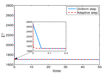
We simulate the growth of a polycrystal in a supercooled liquid with the above random initial liquid density in this example. We begin with examining the efficiency of adaptive time-stepping Algorithm 1 by using different time strategies, i.e., the uniform and adaptive time approaches. At first, the solution is computed until the time $T=50$ with a constant time step $\tau=0.05$ . We then implement the adaptive strategy described in Algorithm 1 to simulate the dynamical process by using the same initial data. The time evolutions of discrete energies and the corresponding time-step sizes are plotted in Figure 3. As can be seen, the adaptive energy curve is practically indistinguishable from that generated by using a small constant step size, and the former exhibits more details owing to the smaller step sizes are used. We note that this simulation takes 1000 uniform time steps with $\tau=0.05$ , while the total number of adaptive time steps is 393. Thus the above numerical results show that the time-stepping adaptive strategy is computationally efficient.

We now use the BDF2 scheme coupled with Algorithm 1 to simulate the growth of a polycrystal in a supercooled liquid. In the second set of simulations, we take the time $T=1000$ and the other parameters are the same as given earlier. The time evolutions of the phase variable are depicted in Figure 4. We see that, the speed of moving interfaces is deeply affected by the initial amplitude, that is, the larger the amplitude $A$ , the faster the polycrystal grows. Also, three different crystal grains grow and become large enough to form grain boundaries eventually. The observed phenomena are in good agreement with the published results [14, 11]. The original energy, mass, and adaptive time steps are shown in Figure 5. As predicted by our theory, the discrete mass is conservative up to a tolerance of $10^{-10}$ . It is seen that the energy has large variations when the time $t\in[0,200]$ , but it dissipates very slowly when the time escapes. The right subplot of Figure 4 shows that small time step sizes are adopted when the energy dissipates fast, and large step sizes are utilized when the energy decreases slowly.

5 Concluding remarks

Under the step ratio constraint S1, we proved the variable-step BDF2 method (1.9) for the PFC model preserves a discrete modified energy dissipation law, which implies the maximum norm bound of numerical solution. The DOC technique was then improved to establish a concise convergence analysis of the variable-step BDF2 method. We proved at the first time that the BDF2 method is convergent in the $L^{2}$ norm under the weak step ratio restriction S1.

In our recent work [32], the DOC technique will be further developed to establish a sharp $L^{2}$ error estimate on the variable-step BDF2 scheme for the molecular beam epitaxial growth model without slope selection. It is expected that the DOC technique would be a useful analysis tool for other variable-step BDF type methods, especially when they are combined with the convex splitting technique or stabilized strategies to achieve unconditionally energy stable in simulating gradient flow problems. We plan to address these issues in further studies.

Acknowledgements

The authors would like to thank Prof. Xiuling Hu, Prof. Yuezheng Gong, and Dr. Lin Wang for their valuable discussions and fruitful suggestions. We also thank the editor and the anonymous referees for their valuable comments and suggestions, which are very helpful for improving the quality of the article.

Appendix A The proof of Lemma 3.2

To facilitate the proof in what follows, we introduce the following matrices

\mathbf{B}_{2}:=\left(\begin{array}[]{cccc}b_{0}^{(1)}&&&\\ b_{1}^{(2)}&b_{0}^{(2)}&&\\ &\ddots&\ddots&\\ &&b_{1}^{(n)}&b_{0}^{(n)}\\ \end{array}\right)_{n\times n}\quad\text{and}\quad\mathbf{\Theta}_{2}:=\left(\begin{array}[]{cccc}\theta_{0}^{(1)}&&&\\ \theta_{1}^{(2)}&\theta_{0}^{(2)}&&\\ \vdots&\vdots&\ddots&\\ \theta_{n-1}^{(n)}&\theta_{n-2}^{(n)}&\cdots&\theta_{0}^{(n)}\\ \end{array}\right)_{n\times n},

where the discrete kernels $b_{n-k}^{(n)}$ and $\theta_{n-k}^{(n)}$ are defined by (1.5) and (1.6), respectively. It follows from the discrete orthogonal identity (1.7) that

\displaystyle\mathbf{\Theta}_{2}=\mathbf{B}_{2}^{-1}.

(A.1)

If the step ratios condition S1 holds, Lemma 2.2 shows that the real symmetric matrix

\displaystyle\mathbf{B}:=\mathbf{B}_{2}+\mathbf{B}_{2}^{T}\quad\text{is positive definite,}

(A.2)

that is, $\boldsymbol{w}^{T}\mathbf{B}\boldsymbol{w}=2\sum_{k=1}^{n}w_{k}\sum_{j=1}^{k}b_{k-j}^{(k)}w_{j}\geq\sum_{k=1}^{n}R(r_{k},r_{k+1})w_{k}^{2}/\tau_{k}$ , where $R(z,s)$ is defined by (2.3) and $\boldsymbol{w}:=\left(w_{1},w_{2},\cdots,w_{n}\right)^{T}$ . According to Lemma 3.1 (I), the real symmetric matrix

\displaystyle\mathbf{\Theta}:=\mathbf{\Theta}_{2}+\mathbf{\Theta}_{2}^{T}\quad\text{is positive definite,}

(A.3)

in the sense of $\boldsymbol{w}^{T}\mathbf{\Theta}\boldsymbol{w}=2\sum_{k=1}^{n}w_{k}\sum_{j=1}^{k}\theta_{k-j}^{(k)}w_{j}>0$ .

Moreover, we define a diagonal matrix $\Lambda_{\tau}:=\text{diag}\left(\sqrt{\tau_{1}},\sqrt{\tau_{2}},\cdots,\sqrt{\tau_{n}}\right)$ and

\displaystyle\widetilde{\mathbf{B}}_{2}:=\Lambda_{\tau}\mathbf{B}_{2}\Lambda_{\tau}=\left(\begin{array}[]{cccc}\tilde{b}_{0}^{(1)}&&&\\ \tilde{b}_{1}^{(2)}&\tilde{b}_{0}^{(2)}&&\\ &\ddots&\ddots&\\ &&\tilde{b}_{1}^{(n)}&\tilde{b}_{0}^{(n)}\\ \end{array}\right)_{n\times n},

(A.8)

where the discrete kernels $\tilde{b}_{0}^{(k)}$ and $\tilde{b}_{1}^{(k)}$ are given by ( $r_{1}\equiv 0$ )

\tilde{b}_{0}^{(k)}=\frac{1+2r_{k}}{1+r_{k}}\quad\text{and}\quad\tilde{b}_{1}^{(k)}=-\frac{r_{k}^{3/2}}{1+r_{k}}\quad\text{for $1\leqslant k\leqslant n$}.

Some results on the matrix $\widetilde{\mathbf{B}}_{2}$ are presented as follows.

Lemma A.1

If the step ratios condition S1 holds, then the minimum eigenvalue of the real symmetric matrix

\displaystyle\widetilde{\mathbf{B}}:=\widetilde{\mathbf{B}}_{2}+\widetilde{\mathbf{B}}_{2}^{T}

(A.9)

can be bounded by

\lambda_{\min}\big{(}\widetilde{\mathbf{B}}\big{)}\geq\min_{1\leq k\leq n}R_{L}\left(r_{k},r_{k+1}\right)\geq 21/40,

where $R_{L}\left(z,s\right)$ is defined by

\displaystyle R_{L}\left(z,s\right):=\frac{2+4z-z^{3/2}}{1+z}-\frac{s^{3/2}}{1+s}\quad\text{for $0\leq z,s<r_{\mathrm{sup}}=\tfrac{3+\sqrt{17}}{2}.$}

(A.10)

Thus $\widetilde{\mathbf{B}}$ is positive definite and there exists a non-singular upper triangular matrix $\mathbf{L}$ such that

\widetilde{\mathbf{B}}=\Lambda_{\tau}\mathbf{B}\Lambda_{\tau}=\mathbf{L}^{T}\mathbf{L}\quad\text{or}\quad\mathbf{B}=\left(\mathbf{L}\Lambda_{\tau}^{-1}\right)^{T}\mathbf{L}\Lambda_{\tau}^{-1}.

Proof Note that, $\partial R_{L}/\partial z=\frac{(1-\sqrt{z})(z+\sqrt{z}+4)}{2(1+z)^{2}}$ . Thus $R_{L}\left(z,s\right)$ is increasing in $(0,1)$ and decreasing in $(1,r_{\mathrm{sup}})$ with respect to $z$ . Also, $R_{L}\left(z,s\right)$ is decreasing with respect to $s$ such that $R_{L}\left(z,s\right)<R_{L}\left(z,0\right)$ for any $s\in(0,r_{\mathrm{sup}})$ . Simple calculations show that

\displaystyle R_{L}\left(z,s\right)\geq\min\big{\{}R_{L}\left(0,r_{\mathrm{sup}}\right),R_{L}\left(r_{\mathrm{sup}},r_{\mathrm{sup}}\right)\big{\}}>21/40\quad\text{for $0\leq z,s<r_{\mathrm{sup}}.$}

(A.11)

For any fixed index $n$ , by using the definition (A.8) of $\widetilde{\mathbf{B}}_{2}$ and the well–known Gerschgorin’s circle theorem, we find that the minimum eigenvalue of $\widetilde{\mathbf{B}}$ can be bounded by

	$\displaystyle\lambda_{\min}\big{(}\widetilde{\mathbf{B}}\big{)}\geq$	$\displaystyle\,\min_{1\leq k\leq n-1}\Big{\{}2\tilde{b}_{0}^{(k)}-\big{\|}\tilde{b}_{1}^{(k)}\big{\|}-\big{\|}\tilde{b}_{1}^{(k+1)}\big{\|},2\tilde{b}_{0}^{(n)}-\big{\|}\tilde{b}_{1}^{(n)}\big{\|}\Big{\}}$
	$\displaystyle=$	$\displaystyle\,\min_{1\leq k\leq n-1}\Big{\{}2\tilde{b}_{0}^{(k)}+\tilde{b}_{1}^{(k)}+\tilde{b}_{1}^{(k+1)},2\tilde{b}_{0}^{(n)}+\tilde{b}_{1}^{(n)}\Big{\}}$
	$\displaystyle=$	$\displaystyle\,\min_{1\leq k\leq n-1}\Big{\{}R_{L}\left(r_{k},r_{k+1}\right),R_{L}\left(r_{n},0\right)\Big{\}}\geq\min_{1\leq k\leq n}R_{L}\left(r_{k},r_{k+1}\right)>21/40,$

where the last estimate follows from (A.11). It also says that the real symmetric matrix $\widetilde{\mathbf{B}}$ is positive definite. Then we complete the proof by noticing the definition (A.2) and applying the standard Cholesky decomposition of $\widetilde{\mathbf{B}}$ .

Lemma A.2

If the step ratios condition S1 holds, the maximum eigenvalue of the real symmetric matrix $\widetilde{\mathbf{B}}_{2}^{T}\widetilde{\mathbf{B}}_{2}$ can be bounded by

\lambda_{\max}\big{(}\widetilde{\mathbf{B}}_{2}^{T}\widetilde{\mathbf{B}}_{2}\big{)}\leqslant\max_{1\leq k\leq n}R_{U}\left(r_{k},r_{k+1}\right)<R_{U}\left(r_{\mathrm{sup}},r_{\mathrm{sup}}\right)<53/5,

where $\widetilde{\mathbf{B}}_{2}$ is defined in (A.8) and $R_{U}\left(z,s\right)$ is defined by

\displaystyle R_{U}\left(z,s\right):=\frac{(1+2z)(1+2z+z^{3/2})}{\left(1+z\right)^{2}}+\frac{s^{3/2}(1+2s+s^{3/2})}{\left(1+s\right)^{2}}\quad\text{for $0\leq z,s<r_{\mathrm{sup}}.$}

(A.12)

Proof Obviously, $R_{U}\left(z,s\right)$ is increasing with respect to the two variables $z$ and $s$ . We have $R_{U}\left(z,s\right)<R_{U}\left(r_{\mathrm{sup}},r_{\mathrm{sup}}\right)<53/5$ . From the definition (A.8) of $\widetilde{\mathbf{B}}_{2}$ , one has

\widetilde{\mathbf{B}}_{2}^{T}\widetilde{\mathbf{B}}_{2}=\left(\begin{array}[]{ccccc}d_{0}^{(1)}&d_{1}^{(2)}&&&\\ d_{1}^{(2)}&d_{0}^{(2)}&d_{1}^{(3)}&&\\ &\ddots&\ddots&\ddots&\\ &&d_{1}^{(n-1)}&d_{0}^{(n-1)}&d_{1}^{(n)}\\ &&&d_{1}^{(n)}&d_{0}^{(n)}\\ \end{array}\right)_{n\times n},

where the discrete kernels $d_{0}^{(k)}$ and $d_{1}^{(k)}$ are given by ( $r_{1}\equiv 0$ )

d_{0}^{(k)}=\Big{(}\frac{1+2r_{k}}{1+r_{k}}\Big{)}^{2}+\frac{r_{k+1}^{3}}{(1+r_{k+1})^{2}}\quad\text{and}\quad d_{1}^{(k)}=-\frac{r_{k}^{3/2}\left(1+2r_{k}\right)}{\left(1+r_{k}\right)^{2}}\quad\text{for $1\leqslant k\leqslant n$}.

For any fixed index $n$ , the Gerschgorin circle theorem gives an upper bound of the maximum eigenvalue of the real symmetric matrix $\widetilde{\mathbf{B}}_{2}^{T}\widetilde{\mathbf{B}}_{2}$ , that is,

	$\displaystyle\lambda_{\max}\big{(}\widetilde{\mathbf{B}}_{2}^{T}\widetilde{\mathbf{B}}_{2}\big{)}\leq$	$\displaystyle\,\max_{1\leq k\leq n-1}\Big{\{}d_{0}^{(k)}-d_{1}^{(k)}-d_{1}^{(k+1)},d_{0}^{(n)}-d_{1}^{(n)}\Big{\}}$
	$\displaystyle=$	$\displaystyle\,\max_{1\leq k\leq n-1}\Big{\{}R_{U}\left(r_{k},r_{k+1}\right),R_{U}\left(r_{n},0\right)\Big{\}}\leq\max_{1\leq k\leq n}R_{U}\left(r_{k},r_{k+1}\right).$

It completes the proof.

Lemma A.3

If S1 holds, then the positive definite matrix $\mathbf{\Theta}=(\mathbf{B}_{2}^{-1})^{T}\mathbf{B}\mathbf{B}_{2}^{-1}$ and

\displaystyle\sum_{k=1}^{n}\sum_{j=1}^{k}\theta_{k-j}^{(k)}w_{k}v_{j}\leq\frac{\varepsilon}{2}\boldsymbol{v}^{T}\mathbf{\Theta}\boldsymbol{v}+\frac{1}{2\varepsilon}\boldsymbol{w}^{T}\mathbf{B}^{-1}\boldsymbol{w}\quad\text{for $\varepsilon>0$}

for any real vectors $\boldsymbol{v}:=\left(v_{1},v_{2},\cdots,v_{n}\right)^{T}$ and $\boldsymbol{w}:=\left(w_{1},w_{2},\cdots,w_{n}\right)^{T}$ .

Proof For any fixed index $n$ , let $\boldsymbol{u}:=\mathbf{\Theta}_{2}\boldsymbol{v}$ . The equality (A.1) gives $\boldsymbol{v}=\mathbf{B}_{2}\boldsymbol{u}$ . In the element-wise sense, one has $u_{k}=\sum_{j=1}^{k}\theta_{k-j}^{(k)}v_{j}$ and $v_{k}=\sum_{j=1}^{k}b_{k-j}^{(k)}u_{j}$ . Then we have

\displaystyle\boldsymbol{v}^{T}\mathbf{\Theta}\boldsymbol{v}=2\sum_{k=1}^{n}\sum_{j=1}^{k}\theta_{k-j}^{(k)}v_{k}v_{j}=2\sum_{k=1}^{n}\sum_{j=1}^{k}b_{k-j}^{(k)}u_{k}u_{j}=\boldsymbol{u}^{T}\mathbf{B}\boldsymbol{u},

(A.13)

and then, by taking $\boldsymbol{u}:=\mathbf{B}_{2}^{-1}\boldsymbol{v}$ ,

\displaystyle\boldsymbol{v}^{T}\left[\mathbf{\Theta}-(\mathbf{B}_{2}^{-1})^{T}\mathbf{B}\mathbf{B}_{2}^{-1}\right]\boldsymbol{v}\equiv 0\quad\text{or}\quad\mathbf{\Theta}=(\mathbf{B}_{2}^{-1})^{T}\mathbf{B}\mathbf{B}_{2}^{-1}.

(A.14)

By virtue of the decomposition $\mathbf{B}=\left(\mathbf{L}\Lambda_{\tau}^{-1}\right)^{T}\mathbf{L}\Lambda_{\tau}^{-1}$ in Lemma A.1, we have

	$\displaystyle\sum_{k=1}^{n}\sum_{j=1}^{k}\theta_{k-j}^{(k)}w_{k}v_{j}=$	$\displaystyle\,\sum_{k=1}^{n}w_{k}u_{k}=\boldsymbol{u}^{T}\boldsymbol{w}=\big{(}\mathbf{L}\Lambda_{\tau}^{-1}\boldsymbol{u}\big{)}^{T}\big{(}\Lambda_{\tau}\mathbf{L}^{-1}\big{)}^{T}\boldsymbol{w}$
	$\displaystyle\leq$	$\displaystyle\,\frac{\varepsilon}{2}\boldsymbol{u}^{T}\big{(}\mathbf{L}\Lambda_{\tau}^{-1}\big{)}^{T}\mathbf{L}\Lambda_{\tau}^{-1}\boldsymbol{u}+\frac{1}{2\varepsilon}\boldsymbol{w}^{T}\big{(}\Lambda_{\tau}\mathbf{L}^{-1}\big{)}\big{(}\Lambda_{\tau}\mathbf{L}^{-1}\big{)}^{T}\boldsymbol{w}$
	$\displaystyle=$	$\displaystyle\,\frac{\varepsilon}{2}\boldsymbol{u}^{T}\mathbf{B}\boldsymbol{u}+\frac{1}{2\varepsilon}\boldsymbol{w}^{T}\Lambda_{\tau}\mathbf{L}^{-1}\big{(}\mathbf{L}^{-1}\big{)}^{T}\Lambda_{\tau}\boldsymbol{w}$
	$\displaystyle=$	$\displaystyle\,\frac{\varepsilon}{2}\boldsymbol{v}^{T}\mathbf{\Theta}\boldsymbol{v}+\frac{1}{2\varepsilon}\boldsymbol{w}^{T}\mathbf{B}^{-1}\boldsymbol{w}\quad\text{for any $\varepsilon>0$,}$

where the Young’s inequality was used in the inequality and the identity (A.13) was applied in the last equality. This completes the proof.

Now we are in position to present the proof of Lemma 3.2.

Proof of Lemma 3.2 To avoid possible confusions, we define the vector norm $\big{|}\!\big{|}\!\big{|}\cdot\big{|}\!\big{|}\!\big{|}$ by $\big{|}\!\big{|}\!\big{|}\boldsymbol{u}\big{|}\!\big{|}\!\big{|}:=\sqrt{\boldsymbol{u}^{T}\boldsymbol{u}}$ and the associated matrix norm $\big{|}\!\big{|}\!\big{|}\textbf{A}\big{|}\!\big{|}\!\big{|}:=\sqrt{\rho\big{(}\textbf{A}^{T}\textbf{A}\big{)}}$ . Lemma A.3 gives

\displaystyle\sum_{k=1}^{n}\sum_{j=1}^{k}\theta_{k-j}^{(k)}w_{k}v_{j}\leq\varepsilon\sum_{k=1}^{n}\sum_{j=1}^{k}\theta_{k-j}^{(k)}v_{k}v_{j}+\frac{1}{2\varepsilon}\boldsymbol{w}^{T}\mathbf{B}^{-1}\boldsymbol{w}\quad\text{for $\varepsilon>0$}.

(A.15)

We will handle the second term at the right side of (A.15). Lemma A.1 shows $\widetilde{\mathbf{B}}=\mathbf{L}^{T}\mathbf{L}$ and $\mathbf{B}^{-1}=\Lambda_{\tau}\mathbf{L}^{-1}\big{(}\mathbf{L}^{-1}\big{)}^{T}\Lambda_{\tau}$ . Moreover, Lemma A.3 gives

\displaystyle\mathbf{\Theta}=

\displaystyle\,(\mathbf{B}_{2}^{-1})^{T}\mathbf{B}\mathbf{B}_{2}^{-1}=(\mathbf{B}_{2}^{-1})^{T}\left(\mathbf{L}\Lambda_{\tau}^{-1}\right)^{T}\mathbf{L}\Lambda_{\tau}^{-1}\mathbf{B}_{2}^{-1}=\left(\mathbf{L}\Lambda_{\tau}^{-1}\mathbf{B}_{2}^{-1}\right)^{T}\mathbf{L}\Lambda_{\tau}^{-1}\mathbf{B}_{2}^{-1}

such that $\boldsymbol{w}^{T}\mathbf{\Theta}\boldsymbol{w}=\big{|}\!\big{|}\!\big{|}\mathbf{L}\Lambda_{\tau}^{-1}\mathbf{B}_{2}^{-1}\boldsymbol{w}\big{|}\!\big{|}\!\big{|}^{2}$ . We apply the definition (A.8) to derive that

	$\displaystyle\boldsymbol{w}^{T}\mathbf{B}^{-1}\boldsymbol{w}=$	$\displaystyle\,\left(\big{(}\mathbf{L}^{-1}\big{)}^{T}\Lambda_{\tau}\boldsymbol{w}\right)^{T}\big{(}\mathbf{L}^{-1}\big{)}^{T}\Lambda_{\tau}\boldsymbol{w}=\big{\|}\!\big{\|}\!\big{\|}\big{(}\mathbf{L}^{-1}\big{)}^{T}\Lambda_{\tau}\boldsymbol{w}\big{\|}\!\big{\|}\!\big{\|}^{2}$
	$\displaystyle=$	$\displaystyle\,\big{\|}\!\big{\|}\!\big{\|}\big{(}\mathbf{L}^{-1}\big{)}^{T}\Lambda_{\tau}\mathbf{B}_{2}\Lambda_{\tau}\mathbf{L}^{-1}\mathbf{L}\Lambda_{\tau}^{-1}\mathbf{B}_{2}^{-1}\boldsymbol{w}\big{\|}\!\big{\|}\!\big{\|}^{2}$
	$\displaystyle\leq$	$\displaystyle\,\big{\|}\!\big{\|}\!\big{\|}\big{(}\mathbf{L}^{-1}\big{)}^{T}\Lambda_{\tau}\mathbf{B}_{2}\Lambda_{\tau}\mathbf{L}^{-1}\big{\|}\!\big{\|}\!\big{\|}^{2}\big{\|}\!\big{\|}\!\big{\|}\mathbf{L}\Lambda_{\tau}^{-1}\mathbf{B}_{2}^{-1}\boldsymbol{w}\big{\|}\!\big{\|}\!\big{\|}^{2}$
	$\displaystyle=$	$\displaystyle\,\big{\|}\!\big{\|}\!\big{\|}\big{(}\mathbf{L}^{-1}\big{)}^{T}\widetilde{\mathbf{B}}_{2}\mathbf{L}^{-1}\big{\|}\!\big{\|}\!\big{\|}^{2}\cdot\boldsymbol{w}^{T}\mathbf{\Theta}\boldsymbol{w}\leq\mathcal{M}_{r}^{(n)}\cdot\boldsymbol{w}^{T}\mathbf{\Theta}\boldsymbol{w},$

where we denote

\displaystyle\mathcal{M}_{r}^{(n)}:=

\displaystyle\,\big{|}\!\big{|}\!\big{|}\mathbf{L}^{-1}\big{|}\!\big{|}\!\big{|}^{4}\big{|}\!\big{|}\!\big{|}\widetilde{\mathbf{B}}_{2}\big{|}\!\big{|}\!\big{|}^{2}=\lambda_{\max}^{2}\big{(}\big{(}\widetilde{\mathbf{B}}^{T}\big{)}^{-1}\big{)}\lambda_{\max}\big{(}\widetilde{\mathbf{B}}_{2}^{T}\widetilde{\mathbf{B}}_{2}\big{)}=\frac{\lambda_{\max}\big{(}\widetilde{\mathbf{B}}_{2}^{T}\widetilde{\mathbf{B}}_{2}\big{)}}{\lambda_{\min}^{2}\big{(}\widetilde{\mathbf{B}}\big{)}}.

(A.16)

Therefore it follows from (A.15) that

\displaystyle\sum_{k=1}^{n}\sum_{j=1}^{k}\theta_{k-j}^{(k)}w_{k}v_{j}\leq\varepsilon\sum_{k=1}^{n}\sum_{j=1}^{k}\theta_{k-j}^{(k)}v_{k}v_{j}+\frac{\mathcal{M}_{r}^{(n)}}{\varepsilon}\sum_{k=1}^{n}\sum_{j=1}^{k}\theta_{k-j}^{(k)}w_{k}w_{j}\quad\text{for $\varepsilon>0$}.

To complete the proof, it remains to show that $\mathcal{M}_{r}^{(n)}$ is uniformly bounded with respect to the level index $n$ . Fortunately, Lemmas A.1 and A.2 confirm that there exists an $n$ -independent constant $\mathcal{M}_{r}:=\max_{n\geq 1}\mathcal{M}_{r}^{(n)}<39$ . Actually, under the weak step-ratio condition S1, one has a rough estimate

\displaystyle\mathcal{M}_{r}=\max_{n\geq 1}\frac{\lambda_{\max}\big{(}\widetilde{\mathbf{B}}_{2}^{T}\widetilde{\mathbf{B}}_{2}\big{)}}{\lambda_{\min}^{2}\big{(}\widetilde{\mathbf{B}}\big{)}}\leq\max_{n\geq 1}\frac{\max_{1\leq k\leq n}R_{U}\left(r_{k},r_{k+1}\right)}{\min_{1\leq k\leq n}R_{L}^{2}\left(r_{k},r_{k+1}\right)}<39.

It completes the proof.

Remark 3 (Improved estimate on the constant $\mathcal{M}_{r}$ )

As noted in [28], the adjacent step ratios take $r_{n}\approx 1$ when the solution varies slowly, and the restriction S1 only takes its effect inside the fast-varying (high gradient) time domains ( $r_{n}<1$ ), in the transition regions from the slow-varying to fast-varying domains ( $r_{n}<1$ ), and in the “fast-to-slow” transition regions ( $r_{n}>1$ ). Then the positive constant $\mathcal{M}_{r}$ in the proof of Lemma 3.2 can be refined by considering three different cases, cf. Remark 1,

(a)

If $0<r_{n}\leq\sqrt{3}-1$ , one can choose $\mathcal{M}_{r}=R_{U}(\sqrt{3}-1,\sqrt{3}-1)/R_{L}^{2}\big{(}0,\sqrt{3}-1\big{)}<1.19;$
(b)

If $\sqrt{3}-1<r_{n}\leq 2$ , then one has $\mathcal{M}_{r}=R_{U}(2,2)/R_{L}^{2}\big{(}2,2\big{)}<3.25;$
(c)

If $2<r_{n}<r_{\mathrm{sup}}$ , one can choose the next step-ratio $0<r_{n+1}\leq 1.45$ (to reduce or slightly enlarge the step size) such that $\mathcal{M}_{r}=R_{U}(r_{\mathrm{sup}},1.45)/R_{L}^{2}\left(r_{\mathrm{sup}},1.45\right)<3.94.$

Always, one can take $\mathcal{M}_{r}=4$ in the adaptive computations.

References

[1] K. Elder, M. Katakowski, M. Haataja, and M. Grant. Modeling elasticity in crystal growth. Phys. Rev. Lett., 88:245701, 2002.
[2] K. Elder and M. Grant. Modeling elastic and plastic deformations in nonequilibrium processing using phase field crystals. Physical Review E, 70:051605, 2004.
[3] N. Provatas, J. Dantzig, B. Athreya, P. Chan, P. Stefanovic, N. Goldenfeld, and K. Elder. Using the phase-field crystal method in the multi-scale modeling of microstructure evolution. JOM, 59:83–90, 2007.
[4] E. Asadi and M. Zaeem. A review of quantitative phase-field crystal modeling of solid-liquid structures. JOM, 67:186–201, 2015.
[5] A. Baskaran, J. Lowengrub, C. Wang, and S. Wise. Convergence analysis of a second order convex splitting scheme for the modified phase field crystal equation. SIAM J. Numer. Anal., 51:2851–2873, 2013.
[6] L. Dong, W. Feng, C. Wang, S. Wise, and Z. Zhang. Convergence analysis and numerical implementation of a second order numerical scheme for the three-dimensional phase field crystal equation. Comput. Math. Appl., 75:1912–1928, 2018.
[7] Q. Li, L. Mei, X. Yang, and Y. Li. Efficient numerical schemes with unconditional energy stabilities for the modified phase field crystal equation. Adv. Comput. Math., 45:1551–1580, 2019.
[8] Z. Liu and X. Li. Efficient modified stabilized invariant energy quadratization approaches for phase-field crystal equation. Numer. Algo., 2019. Doi:10.1007/s11075-019-00804-9.
[9] X. Jing and Q. Wang. Linear second order energy stable schemes for phase field crystal growth models with nonlocal constraints. Comput. Math. Appl., 79:764–788, 2020.
[10] Z. Zhang, Y. Ma, and Z. Qiao. An adaptive time-stepping strategy for solving the phase field crystal model. J. Comput. Phys., 249:204–215, 2013.
[11] X. Yang and D. Han. Linearly first- and second-order, unconditionally energy stable schemes for the phase field crystal model. J. Comput. Phys., 330:1116–1134, 2017.
[12] S. Wise, C. Wang, and J. Lowengrub. An energy-stable and convergent finite-difference scheme for the phase field crystal equation. SIAM J. Numer. Anal., 47:2269–2288, 2009.
[13] C. Wang and S. Wise. An energy stable and convergent finite-difference scheme for the modified phase field crystal equation. SIAM J. Numer. Anal., 49:945–969, 2011.
[14] Y. Li and J. Kim. An efficient and stable compact fourth-order finite difference scheme for the phase field crystal equation. Comput. Methods Appl. Mech. Eng., 319:194–216, 2017.
[15] Y. Yan, W. Chen, C. Wang, and S. Wise. A second-order energy stable BDF numerical scheme for the Cahn-Hilliard equation. Comm. Comput. Phys., 23:572–602, 2018.
[16] K. Cheng, W. Feng, C. Wang, and S. Wise. An energy stable fourth order finite difference scheme for the Cahn-Hilliard equation. J. Comput. Appl. Math., 362:574–595, 2019.
[17] K. Cheng, C. Wang, and S. Wise. An energy stable BDF2 Fourier pseudo-spectral numerical scheme for the square phase field crystal equation. Comm. Comput. Phys., 26:1335–1364, 2019.
[18] C. Xu and T. T. Tang. Stability analysis of large time-stepping methods for epitaxial growth models. SIAM J. Numer. Anal., 44:1759–1779, 2006.
[19] J. Shen and X. Yang. Numerical approximations of Allen-Cahn and Cahn-Hilliard equations. Discrete. Contin. Dyn. Sys., 28:1669–1691, 2010.
[20] J. Shen, T. Tang, and J. Yang. On the maximum principle preserving schemes for the generalized Allen-Cahn equation. Commu. Math. Sci., 14:1517–1534, 2016.
[21] Gong. Y. and J. Zhao. Energy-stable Runge-Kutta schemes for gradient flow models uing the energy quadratization approach. Appl. Math. Lett., 94:224–231, 2019.
[22] J. Xu, Y. Li, S. Wu, and A. Bousquet. On the stability and accuracy of partially and fully implicit schemes for phase field modeling. Comput. Methods Appl. Mech. Eng., 345:826–853, 2019.
[23] H. Gomez and T. Hughes. Provably unconditionally stable, second-order time-accurate, mixed variational methods for phase-field models. J. Comput. Phys., 230:5310–5327, 2011.
[24] Z. Qiao, Z. Zheng, and T. Tang. An adaptive time-stepping strategy for the molecular beam epitaxy models. SIAM J. Sci. Comput., 22:1395–1414, 2011.
[25] R. D. Grigorieff. Stability of multistep-methods on variable grids. Numer. Math., 42:359–377, 1983.
[26] J. Becker. A second order backward difference method with variable steps for a parabolic problem. BIT Numerical Mathematics, 38:644–662, 1998.
[27] W. Chen, X. Wang, Y. Yan, and Z. Zhang. A second order BDF numerical scheme with variable steps for the Cahn-Hilliard equation. SIAM J. Numer. Anal., 57:495–525, 2019.
[28] H.-L. Liao and Z. Zhang. Analysis of adaptive BDF2 scheme for diffusion equations. Math. Comp., 2020, to appear.
[29] J. Shen, T. Tang, and L. Wang. Spectral methods: Algorithms, analysis and applications. Springer-Verlag, Berlin Heidelberg, 2011.
[30] S. Gottlieb and C. Wang. Stability and convergence analysis of fully discrete Fourier collocation spectral method for 3-D viscous Burgers’ equation. J. Sci. Comput., 53:102–128, 2012.
[31] K. Cheng, C. Wang, S. Wise, and X. Yue. A second-order, weakly energy-stable pseudo-spectral scheme for the Cahn-Hilliard equation and its solution by the homogeneous linear iteration method. J. Sci. Comput., 69:1083–1114, 2016.
[32] H-L. Liao, X. Song, T. Tang, and T. Zhou. Analysis of the second order BDF scheme with variable steps for the molecular beam epitaxial model without slope selection. preprint, 2019. submitted to pubilication.

	$\displaystyle\frac{\,\mathrm{d}^{2}G}{\,\mathrm{d}\lambda^{2}}[z+\lambda\psi]\Big{\|}_{\lambda=0}=$	$\displaystyle\,b_{0}^{(n)}\big{\\|}\psi\big{\\|}_{-1}^{2}+\big{\\|}(1+\Delta_{h})\psi\big{\\|}^{2}+3\big{\\|}z\psi\big{\\|}^{2}-\epsilon\big{\\|}\psi\big{\\|}^{2}$
	$\displaystyle\geq$	$\displaystyle\,\big{(}b_{0}^{(n)}-\frac{3\epsilon}{2}\big{)}\big{\\|}\psi\big{\\|}_{-1}^{2}+\frac{2}{3}\big{\\|}(1+\Delta_{h})\psi\big{\\|}^{2}+3\big{\\|}z\psi\big{\\|}^{2}>0,$

$\displaystyle\mathbb{I}_{21}$	$\displaystyle=\left\\|\Delta\left(\Phi^{3}-\Phi_{M}^{3}\right)\right\\|=\left\\|I_{M}\left(\Delta\left(\Phi^{3}-\Phi_{M}^{3}\right)\right)\right\\|_{L^{2}}$
	$\displaystyle\leq\left\\|I_{M}\left(\Delta\Phi^{3}\right)-\Delta\Phi^{3}\right\\|_{L^{2}}+\left\\|\Delta\left(\Phi^{3}-\Phi_{M}^{3}\right)\right\\|_{L^{2}}+\left\\|\Delta\Phi_{M}^{3}-I_{M}\left(\Delta\Phi_{M}^{3}\right)\right\\|_{L^{2}}$
	$\displaystyle\leq C_{\phi}h^{m}\left\\|\Phi^{3}\right\\|_{H^{m+2}}+C_{\phi}h^{m}\left\\|\Phi_{M}^{3}\right\\|_{H^{m+2}}+\left\\|\Delta\left(\Phi^{3}-\Phi_{M}^{3}\right)\right\\|_{L^{2}}$
	$\displaystyle\leq C_{\phi}h^{m}\left\\|\Phi\right\\|_{H^{m+2}}^{3}+C_{\phi}h^{m}\left\\|\Phi_{M}\right\\|_{H^{m+2}}^{3}+\left\\|\Delta\left(\Phi^{3}-\Phi_{M}^{3}\right)\right\\|_{L^{2}},$	(3.11)

An adaptive BDF2 implicit time-stepping method for the phase field crystal model

Abstract

1 Introduction

2 Energy dissipation law and solvability

2.1 Spatial discretization and preliminary results

2.2 Unique solvability

Lemma 2.1

Theorem 2.1

2.3 Energy dissipation law

Lemma 2.2

Theorem 2.2

Remark 1

Lemma 2.3

3 L2L^{2} norm error estimate

3.1 Some properties of DOC kernels

Lemma 3.1

Lemma 3.2

Lemma 3.3

3.2 Convolutional consistency in time

Lemma 3.4

Remark 2

3.3 Convergence analysis

Lemma 3.5

Theorem 3.1

Stage 1: Consistency analysis of semi-discrete projection

Stage 2: L2L^{2} norm error of fully discrete system

4 Numerical experiments

4.1 Tests on random time meshes

Example 4.1

4.2 Numerical comparisons

Example 4.2

4.3 Adaptive time-stepping strategy

4.4 Growth of a polycrystal

Example 4.3

5 Concluding remarks

Acknowledgements

Appendix A The proof of Lemma 3.2

Lemma A.1

Lemma A.2

Lemma A.3

Remark 3 (Improved estimate on the constant ℳr\mathcal{M}_{r})

References

An adaptive BDF2 implicit time-stepping method
for the phase field crystal model

3 $L^{2}$ norm error estimate

Stage 2: $L^{2}$ norm error of fully discrete system

Remark 3 (Improved estimate on the constant $\mathcal{M}_{r}$ )