An accurate and efficient Ehrenfest dynamics approach for calculating linear and nonlinear electronic spectra
Abstract
Linear and nonlinear electronic spectra provide an important tool to probe the absorption and transfer of electronic energy. Here we introduce a pure state Ehrenfest approach to obtain accurate linear and nonlinear spectra that is applicable to systems with large numbers of excited states and complex chemical environments. We achieve this by representing the initial conditions as sums of pure states and unfolding multi-time correlation functions into the Schrödinger picture. By doing this we show that one can obtain significant improvements in accuracy over the previously used projected Ehrenfest approach and that these benefits are particularly pronounced in cases where the initial condition is a coherence between excited states. While such initial conditions do not arise when calculating linear electronic spectra, they play a vital role in capturing multidimensional spectroscopies. We demonstrate the performance of our method by showing that it is able to quantitatively capture the exact linear, 2DES, and pump-probe spectra for a Frenkel exciton model in slow bath regimes and is even able to reproduce the main spectral features in fast bath regimes.
I Introduction
Nonlinear optical spectroscopy is a powerful tool for probing the structure and dynamics of chemical systems Ginsberg, Cheng, and Fleming (2009); Cho (2008); Khalil, Demirdöven, and Tokmakoff (2003), and it typically provides significantly more information than its linear counterparts. For example, 2D electronic spectroscopy (2DES) Hybl et al. (1998); Mukamel (1995) is frequently used to elucidate inter-chromophoric couplings, energy transfer and relaxation processes, and environmental effects in systems such as photosynthetic molecular aggregates with femtosecond time resolution Brixner et al. (2005); Engel et al. (2007); Dostál et al. (2012); Abramavicius and Mukamel (2010). However, interpreting these spectra in terms of the specific molecular structures and motions that give rise to the electronic states and their relaxation pathways often requires the assistance of simulations to disentangle spectral features such as short-time coherent oscillations and long-time population decay pathways. Accurately and efficiently simulating 2DES signals from atomistic simulations and uncovering how they arise from the underlying quantum dynamics of the nuclear and electronic states remains a significant challenge.
Simulating nonlinear optical spectra requires obtaining higher-order response functions and hence the number of methods that have successfully been applied to generate them is significantly more limited than for the less computationally demanding linear spectra. Exact methods such as the Hierarchical Equations of Motion (HEOM) Tanimura and Kubo (1989); Ishizaki and Tanimura (2007); Kreisbeck et al. (2011); Chen et al. (2010) and multiconfiguration time-dependent Hartree (MCTDH) Meyer (2011); Schulze et al. (2017) provide important insights and benchmarks for approximate methods. However, the desire to treat large condensed-phase systems containing many electronic states with a fully atomistic treatment of the nuclear motions and even on-the-fly evaluation of the electronic surfaces has spurred the recent development of approximate dynamics methods. When approximate methods are used, 2DES has been shown to provide a much stricter test of the quantum dynamics method employed than linear electronic spectroscopy. For example, when using Redfield theoryREDFIELD (1965); Bloch (1957) it has been shown that in parameter regimes where the linear electronic spectrum can be quantitatively captured, the 2DES spectrum significantly deviates from the exact results Fetherolf and Berkelbach (2017), although this can be somewhat alleviated by freezing the low-frequency bath modes.Montoya-Castillo, Berkelbach, and Reichman (2015); Fetherolf and Berkelbach (2017)
Trajectory-based methods provide a particularly appealing approach to simulate 2DES since they are typically compatible with a fully atomistic treatment of the nuclear motions and even on-the-fly evaluation of the electronic surfaces on which the nuclei evolve. Many recent applications of trajectory-based methods to 2DES have been based on semiclassical treatments of the Meyer-Miller-Stock-Thoss Meyer and Miller (1979); Stock and Thoss (1997) mapping of the electronic degrees of freedom. In particular, the partially linearized density matrix (PLDM) approach Huo and Coker (2011) and its more recent spin-PLDM variant Mannouch and Richardson (2020a, b) have been shown to produce accurate 2DES spectra in parameter regimes where perturbative methods break down Provazza et al. (2018); Mannouch and Richardson (2022). Further work has shown how mapping-based semiclassical methods can be used to simulate 2DES beyond the perturbative treatment of the field-matter interaction Gao and Geva (2020). The optimized mean trajectory approach has also been recently coupled with trajectories based on the Meyer-Miller Hamiltonian to compute two-dimensional vibrational-electronic spectra Polley and Loring (2021); Loring (2022). Other trajectory-based approaches include the numerical integration of the Schrodinger equation (NISE) Jansen and Knoester (2006); Liang and Jansen (2012); Torii (2006) and the stochastic Liouville Equation methods Jansen, Zhuang, and Mukamel (2004); Jansen et al. (2005), which involve an explicit treatment of the bath degrees of freedom but do not account for the back-reaction of the electronic degrees of freedom on the bath, leading to inaccuracies in linear and nonlinear spectra. To correct this, NISE has been combined with the fewest switches surface hopping approach, allowing it to incorporate the quantum back-reaction on the bath and thus improve its accuracy.Tempelaar et al. (2013)
Here, we present an accurate method to simulate 2DES using Ehrenfest dynamics and contrast it with a previously reported method detailed in Ref. van der Vegte et al., 2013. By applying our method, we show that significantly more accurate 2DES spectra can be obtained from Ehrenfest dynamics if one uses an appropriate initialization of coherence and mixed states. In particular, we express all initial conditions as sums of pure states, which have important implications for the accuracy of the resulting dynamics and allow the simulation to be done unambiguously in either the wavefunction or density matrix formulations of Ehrenfest theory. We show that when formulated in this way, Ehrenfest theory can closely reproduce the HEOM result, and that this result is not achieved when initialization is not done from pure states.
II Pure State and Projected Ehrenfest Methods
It has previously been shown that in the density matrix formulation of the Ehrenfest method Kapral and Ciccotti (1999), a carefully constructed initialization is required to obtain unambiguous results because density matrices initialized from non-pure states do not yield unique dynamics Montoya-Castillo and Reichman (2016). Conversely, the wavefunction formulation of Ehrenfest does not suffer from this problem because all initial conditions are automatically pure states. Our approach to the density matrix formulation of Ehrenfest avoids this previously reported ambiguity by expanding any given initial density matrix as a sum of pure states,
| (1) |
For an arbitrary initial density matrix , the pure state decomposition can be accomplished as follows:
| (2) |
where
| (3) |
are pure states. Here we will refer to this approach as pure state Ehrenfest and contrast it with the unmodified alternative, which we refer to as projected Ehrefest, where all initial conditions are propagated directly without having been decomposed into pure states.
III Simulation Details: Frenkel exciton model
We consider a Frenkel exciton model of coupled chromophores where the full matter Hamiltonian is
| (4) |
Here, is the system Hamiltonian, is the bath Hamiltonian, and is the system-bath coupling. The system Hamiltonian, , consists of individual chromophores, each with a site energy , that couple electronically via the transfer integrals :
| (5) |
The bath Hamiltonian, , consists of independent sets of phonon modes coupled to each chromophore. It is expressed in terms of the phonon mode frequencies and their mass-weighted momenta and coordinates and as:
| (6) |
Each chromophore site is linearly coupled to its local bath of phonon modes, such that takes the form
| (7) |
where is the coupling strength of the phonon mode attached to chromophore . The characteristics of the baths and their effect on the chromophores are specified via the spectral density,
| (8) |
All chromophore sites are assumed to have identical spectral densities (). Here, we use an Ohmic spectral density with a Lorentzian cutoff (Debye),
| (9) |
where is the bath cut-off frequency and is the reorganization energy.
To obtain linear and non-linear spectra, we treat the light-matter interaction perturbatively Mukamel (1995), i.e.,
| (10) |
where is the classical electric field and is the total dipole operator,
| (11) |
We consider a system of two coupled chromophores with cm-1, cm-1, and 100 cm-1, consistent with that used in previous studies Ishizaki and Fleming (2009); Fetherolf and Berkelbach (2017). In this system, there are four states, all of which are accessible: the ground state, two singly excited states, and one doubly excited state. We report results for two sets of bath parameters: a slow bath with a relaxation time fs and a fast bath with a relaxation time = 17.7 fs, both at cm-1. Each bath was discretized using 300 phonon modes via the method employed in Ref. Berkelbach, Reichman, and Markland, 2012 that is designed to yield the exact reorganization energy regardless of the number of modes used. The reorganization energy was set to 50 cm-1. All spectra were calculated with a transition dipole matrix where . The slow bath parameter regime was previously investigated via HEOM and Redfield theory and its frozen mode variant in Ref. Fetherolf and Berkelbach, 2017.
Our HEOM and projected Ehrenfest calculations were conducted using the python package pyrho Berkelbach et al. (2020). For the HEOM calculations, converged results for the regimes studied here were obtained by employing the high-temperature approximation, i.e. using zero Matsubara frequencies (), and truncating the auxiliary density matrices at . Both the HEOM and projected Ehrenfest equations of motion were propagated using a fourth-order Runge-Kutta integrator, while the pure state Ehrenfest method was propagated via the split Liouvillian method, allowing for the use of larger time steps. In the slow bath parameter regime, we used time steps of 10 fs for HEOM and 2 fs for both versions of Ehrenfest, while in the fast bath parameter regime, we used a time step of 2.5 fs for HEOM and 10 fs for pure state Ehrenfest. The linear spectra were generated using 20000 trajectories of length 400 fs, while the nonlinear spectra used 20000 trajectories of length 300 fs for the slow bath regime and 200 fs for the fast bath regime.
IV Results
Here we compare the Ehrenfest results for both the linear and nonlinear optical spectra of the Frenkel exciton model outlined in Sec. III to spectra obtained using the numerically exact HEOM approach. We demonstrate that, while in linear absorption spectra the differences between pure state and projected Ehrenfest are subtle, they become much more pronounced for nonlinear spectra.
IV.1 Linear Optical Spectroscopy

Linear absorption spectra can be obtained from the Fourier transform of the first-order response function, Mukamel (1995),
| (12) |
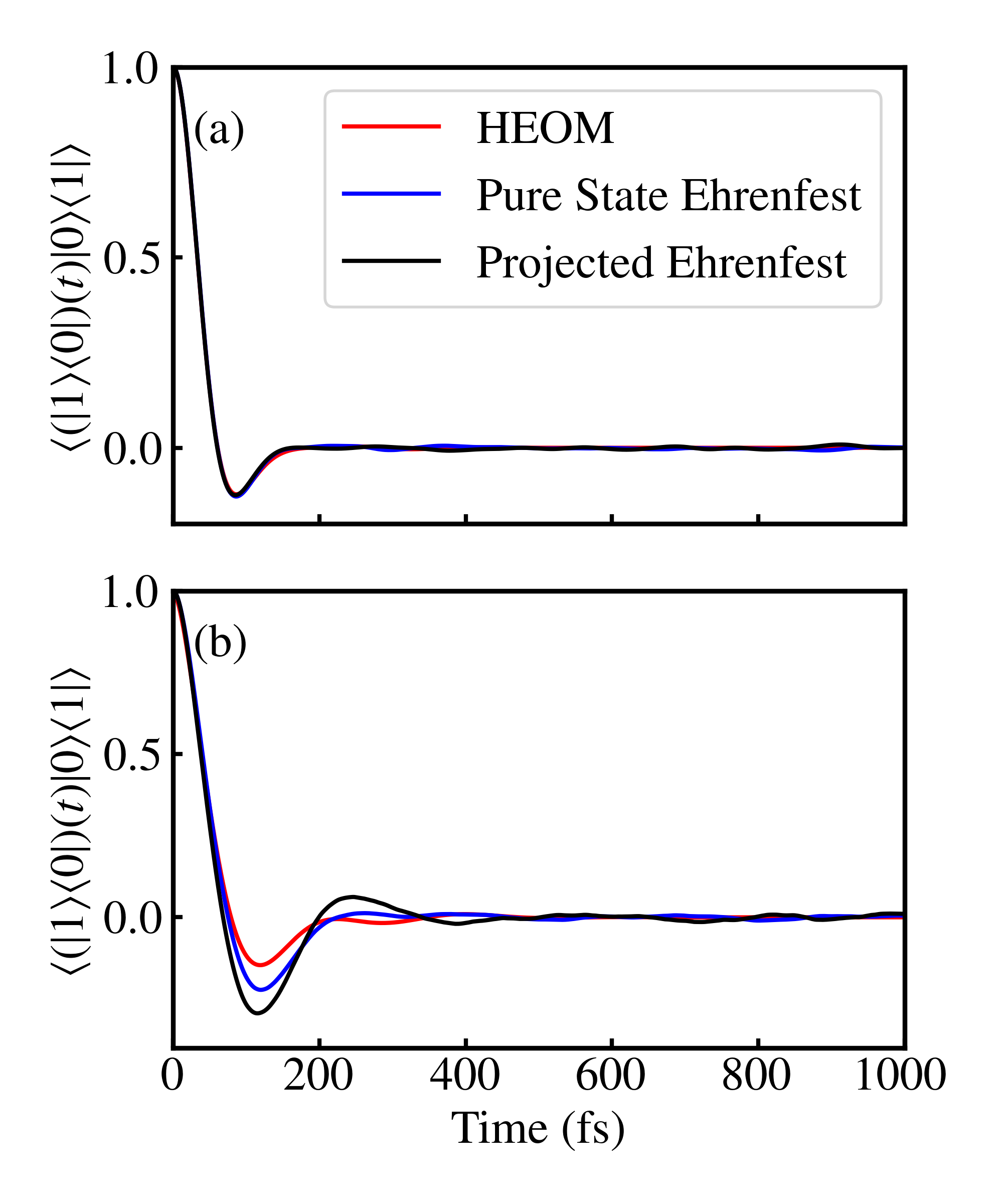
Applying the dipole operator at results in an optical coherence between the ground state and singly excited states, . This initial condition can be represented either as an unmodified projected state (i.e., ) or as a sum of pure states. Absorption spectra computed via pure state Ehrenfest, projected Ehrenfest, and the numerically exact HEOM for both the fast and slow bath parameter regimes are shown in Fig. 1. In the slow bath regime (Fig. 1 (a)), where Ehrenfest theory is expected to be accurate, both projected Ehrenfest and pure state Ehrenfest quantitatively reproduce the HEOM result. In the fast bath parameter regime (Fig. 1 (b)), despite qualitative agreement with the HEOM result, there are small inaccuracies for both Ehrenfest methods, with the pure state Ehrenfest method giving a more accurate result than the projected Ehrenfest method. These results can be explained by examining the dynamics arising from the coherence initial condition, shown in Figs. 2 (a) and (b). is one of the coherence initial conditions (the others being and their complex conjugates) that is propagated to give rise to the first-order response function, . In the slow bath regime, there is near quantitative agreement between both versions of Ehrenfest and the HEOM result, while in the fast bath regime, there are more pronounced differences, with the pure state Ehrenfest dynamics matching the HEOM result more closely and the projected Ehrenfest result being underdamped. These differences mirror and point to the source of inaccuracies in the absorption spectra for the fast bath parameter regime. The overall similarity in coherence dynamics across different methods (Fig. 2) also reveals why the linear spectra appear to be relatively insensitive to the initialization scheme used for Ehrenfest dynamics: the dynamics starting from a density matrix corresponding to a coherence with the ground state are not as sensitive to the initialization scheme. The relative insensitivity of the linear absorption spectra to methods that inaccurately treat coherence dynamics has previously been observed for Redfield theory, which was shown to yield accurate linear absorption spectra despite getting incorrect population dynamics Fetherolf and Berkelbach (2017), albeit with a different dynamical method rooted in perturbation theory.
IV.2 Nonlinear Optical Spectroscopy
Two-dimensional electronic spectra offer a much stricter test than absorption spectroscopy of a method’s accuracy because they require one to correctly capture both the population and coherence dynamics for a wider range of initial conditions.

2DES spectra can be obtained from a Fourier transform over the rephasing () and non-rephasing () terms of third-order response function under the rotating wave approximation Mukamel (1995),
| (13) |
where
| (14) |
include the ground state bleaching, stimulated emission, and excited state absorption contributions, and
| (15) |
Here, is the Liouville-space propagator and
| (16) |
A procedure for obtaining the third-order response function from Ehrenfest dynamics was previously outlined in Ref. van der Vegte et al., 2013, which employs ensemble averages over the ground state wavefunction, . In this scheme, the dipole operator is applied via a product with individual dipole matrix elements, time propagation is done only over select population states, and the effect of coherences is modeled via an average over two wavefunctions formed from the ket and bra. However, the use of specific dipole matrix elements as well as time-propagation over select population states make it difficult to generalize that method to arbitrary systems with multiple quantum states. Here, we present a generalizable method that exploits the linearity of density matrices to compute third-order response functions as follows:
-
1.
Apply the first dipole operator to at and split the resultant density matrix into 4 pure states as described in Section II. Via the Condon approximation, the bath degrees of freedom are untouched by the dipole operator and are initially sampled from the Wigner transform of the Boltzmann distribution on the ground state. Each resultant pure state inherits its own copy of the bath. Propagate states and their corresponding baths independently through .
-
2.
Apply the second dipole operator at , this time to all 4 propagated states. This operation usually results in a new set of non-pure states, which are subsequently split into 4 of their respective pure states, bringing the total number of branches to 16. Each branch adopts a copy of bath coordinates and momenta from its parent branch, ensuring continuity from . Propagate the pure states and baths independently through the waiting time, .
-
3.
Apply the third dipole operator at to the 16 propagated states. This splits them again into a total of 64 branches, each a pure state. Propagate all branches through .
-
4.
Consolidate all 64 branches at and apply the final dipole operator to obtain the third-order response function.
Multiple instances of this procedure are run in order to average over an ensemble of initial bath states. From the above, it is clear that the pure state Ehrenfest method requires more sampling than projected Ehrenfest, which does not involve any splitting of initial conditions into pure states. As we will see below, this splitting into pure states is required to obtain accurate 2DES spectra. The procedure can also be trivially parallelized since all trajectories in the scheme run independently. Additionally, as demonstrated in Section II, we decompose each initial density matrix as a sum of only 4 pure states in the same Liouville space.
An alternative method for obtaining accurate Ehrenfest dynamics from non-pure state density matrices is outlined in our previous work in the Appendices of Ref. Pfalzgraff et al., 2019, and it involves stochastically sampling an auxiliary wavefunction. For example, the initial condition would be obtained from
| (17) |
where is a parameter that is sampled over the range . In this stochastic scheme, sampling is required both over values of and initial positions and momenta of the bath. In the context of a third-order response function, would require fresh sampling every time a measurement is made (i.e., at times , , and ) because the auxiliary wavefunction would otherwise return incorrect dynamics. In contrast, the pure state Ehrenfest method detailed above only requires the usual sampling over initial bath conditions, which can be done once at since the baths are continuous through .


Fig. 3 shows the 2DES spectra obtained from both the pure state and projected forms of Ehrenfest and how they compare to the HEOM spectra. The response functions used to obtain the Ehrenfest spectra were truncated (windowed using a step function) as outlined in the SI Sec. LABEL:sec:third_order_truncation. From this, we observe that pure state Ehrenfest recovers almost quantitative agreement with the HEOM result, with just a slight deterioration as the waiting time increases. In contrast, projected Ehrenfest yields much worse agreement with the HEOM spectrum. While most of the spectral features from the HEOM spectrum are present at , the projected Ehrenfest spectrum becomes progressively worse as increases and bears little resemblance to the HEOM result by the time fs.
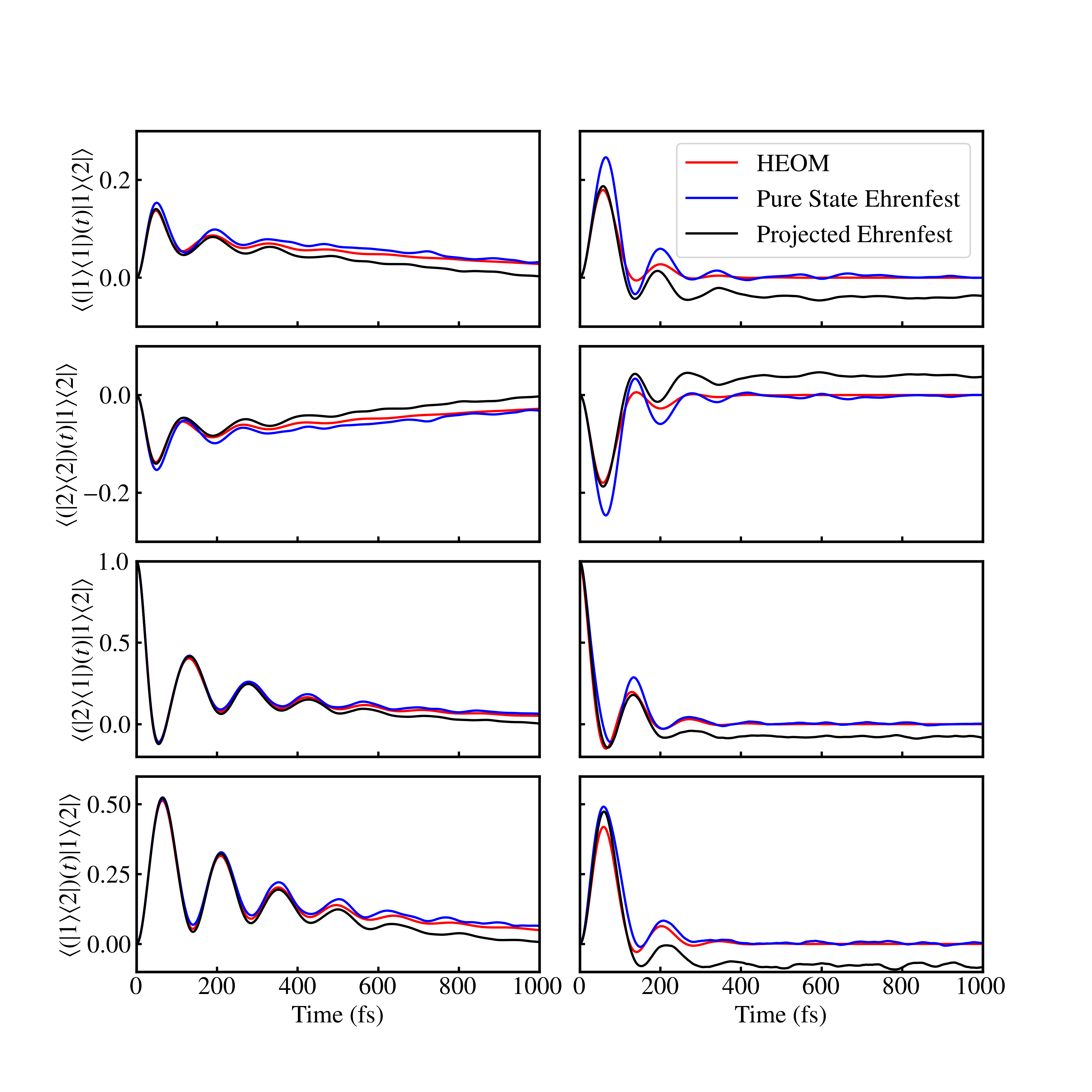
The poor performance of the projected Ehrenfest method can be tracked down to discrepancies in the contributions of the response function. Figs. 4 and 5 illustrate this using plots of , with the rest of the contributions of the response function being shown in SI Figs. LABEL:fig:phi_1_slow- LABEL:fig:phi_6_fast. Here, we observe that, as expected, pure state Ehrenfest accurately reproduces the HEOM result while projected Ehrenfest fails to do so, and that the discrepancy is much more striking in the imaginary part of the response function. These discrepancies can be further traced to the single-time dynamics obtained from coherence initial conditions between excited states. Since the Frenkel exciton model is in the global ground state at , such coherence states can only be obtained when the dipole operator is applied multiple times, as is the case when computing the third-order response. As such, the dynamics of coherence initial conditions between excited states (e.g. ) are relevant to nonlinear spectra but not linear spectra. Figure 6 shows both the population and coherence dynamics for . In both the slow and fast bath parameter regimes, we see from the first two rows that the population dynamics obtained from pure state Ehrenfest more closely match the HEOM result, especially at longer times. In contrast, the projected Ehrenfest result matches the HEOM result until 200 fs, after which there are notable deviations. This poor performance of projected Ehrenfest is also observed to a lesser extent in the coherence dynamics of the initial state (bottom two rows of Fig. 6). We emphasize that the coherence dynamics presented here are distinct from those involved in the absorption spectra since they do not involve the ground state. The worsening performance of projected Ehrenfest with time in reproducing the dynamics arising from also explains why the respective 2DES spectrum degrades progressively as the waiting time increases (Fig. 3). As such, the differences in the performance between projected and pure state Ehrenfest can be attributed to inaccuracies in the projected Ehrenfest dynamics when populations, and coherences to a lesser extent, arise from an initial condition of coherences between two excited states.
Pump-probe spectra, generated by integrating over , are shown in Fig. 7. The results here mirror those of the 2DES spectrum, where the pure state Ehrenfest method accurately reproduces the HEOM result, albeit with slightly higher peaks at 200 cm-1 for 200 fs. In contrast, while the projected Ehrenfest method yields accurate results at , the accuracy of the pump-probe spectra degrades at 200 fs, with the peak around 200 cm-1 losing definition.

Next we examine how well pure state Ehrenfest performs in a more challenging fast bath regime. Fig. 8 shows 2DES spectra for the fast bath parameters computed via HEOM and pure state Ehrenfest. The range of values for (0 - 150 fs) is more limited here than in the slow bath regime because we observed virtually no change in the 2DES spectrum beyond 200 fs (see SI Figure LABEL:fig:fast_bath_extended). As with the slow bath parameter regime, the pure state Ehrenfest response functions were truncated before being Fourier transformed to produce the 2DES spectra (see SI Sec. LABEL:sec:third_order_truncation). In this more challenging regime, pure state Ehrenfest does not perform as well as it did for the slow bath parameters. This is not surprising, as it aligns with the well-known deficiencies of the Ehrenfest method, which struggles to capture the correct dynamics in the limit of fast nuclei. Nonetheless, it is able to qualitatively capture most of the features present in the HEOM spectrum. This result is corroborated by the pump-probe spectra shown in Fig. 9.


V Conclusion
Here we have introduced the pure state Ehrenfest method to obtain linear and nonlinear spectra. We have shown that exploiting the linearity of the density matrix to express all initial conditions as sums of pure states is essential to obtaining accurate coherence dynamics. In particular, while our approach provides modest improvements over projected Ehrenfest in computing linear spectra, it is able to dramatically improve the accuracy with which nonlinear spectra (2DES and pump-probe) can be obtained, especially at longer waiting times. The physical origin of this improvement arises from the ability of our pure state Ehrenfest approach to much more accurately capture the dynamics when the initial condition is a coherence between excited states. These conditions do not occur when calculating the linear spectra (where all the initial density matrices are coherences with the ground state) but play a vital role in obtaining the higher-order response functions needed to capture nonlinear spectroscopy. We have shown that pure state Ehrenfest gives excellent agreement with the exact linear and 2DES spectra in the slow bath regime where the Ehrenfest method is expected to be accurate and have also demonstrated that it still provides good results in a faster bath regime and preserves the qualitative features observed in the exact spectra. These results suggest that the pure state Ehrenfest approach provides a tractable and accurate approach to calculate nonlinear spectra for multichromophoric systems in a wide range of chemical environments.
References
References
- Ginsberg, Cheng, and Fleming (2009) N. S. Ginsberg, Y.-C. Cheng, and G. R. Fleming, Accounts of Chemical Research 42, 1352 (2009).
- Cho (2008) M. Cho, Chemical Reviews 108, 1331 (2008).
- Khalil, Demirdöven, and Tokmakoff (2003) M. Khalil, N. Demirdöven, and A. Tokmakoff, The Journal of Physical Chemistry A 107, 5258 (2003).
- Hybl et al. (1998) J. D. Hybl, A. W. Albrecht, S. M. G. Faeder, and D. M. Jonas, Chemical Physics Letters 297, 307 (1998).
- Mukamel (1995) S. Mukamel, Principles of Nonlinear Optical Spectroscopy, Oxford series in optical and imaging sciences (Oxford University Press, 1995).
- Brixner et al. (2005) T. Brixner, J. Stenger, H. M. Vaswani, M. Cho, R. E. Blankenship, and G. R. Fleming, Nature 434, 625 (2005).
- Engel et al. (2007) G. S. Engel, T. R. Calhoun, E. L. Read, T.-K. Ahn, T. Mančal, Y.-C. Cheng, R. E. Blankenship, and G. R. Fleming, Nature 446, 782 (2007).
- Dostál et al. (2012) J. Dostál, T. Mančal, R. nas Augulis, F. Vácha, J. Pšenčík, and D. Zigmantas, Journal of the American Chemical Society 134, 11611 (2012).
- Abramavicius and Mukamel (2010) D. Abramavicius and S. Mukamel, The Journal of Chemical Physics 133, 184501 (2010).
- Tanimura and Kubo (1989) Y. Tanimura and R. Kubo, Journal of the Physical Society of Japan 58, 101 (1989).
- Ishizaki and Tanimura (2007) A. Ishizaki and Y. Tanimura, The Journal of Physical Chemistry A 111, 9269 (2007).
- Kreisbeck et al. (2011) C. Kreisbeck, T. Kramer, M. Rodríguez, and B. Hein, Journal of Chemical Theory and Computation 7, 2166 (2011).
- Chen et al. (2010) L. Chen, R. Zheng, Q. Shi, and Y. Yan, The Journal of Chemical Physics 132, 024505 (2010).
- Meyer (2011) H.-D. Meyer, Wiley Interdisciplinary Reviews: Computational Molecular Science 2, 351 (2011).
- Schulze et al. (2017) J. Schulze, M. F. Shibl, M. J. Al-Marri, and O. Kühn, Chemical Physics 497, 10 (2017).
- REDFIELD (1965) A. REDFIELD, in Advances in Magnetic Resonance (Elsevier, 1965) pp. 1–32.
- Bloch (1957) F. Bloch, Physical Review 105, 1206 (1957).
- Fetherolf and Berkelbach (2017) J. H. Fetherolf and T. C. Berkelbach, The Journal of Chemical Physics 147, 244109 (2017).
- Montoya-Castillo, Berkelbach, and Reichman (2015) A. Montoya-Castillo, T. C. Berkelbach, and D. R. Reichman, The Journal of Chemical Physics 143, 194108 (2015).
- Meyer and Miller (1979) H.-D. Meyer and W. H. Miller, The Journal of Chemical Physics 70, 3214 (1979).
- Stock and Thoss (1997) G. Stock and M. Thoss, Physical Review Letters 78, 578 (1997).
- Huo and Coker (2011) P. Huo and D. F. Coker, The Journal of Chemical Physics 135, 201101 (2011).
- Mannouch and Richardson (2020a) J. R. Mannouch and J. O. Richardson, The Journal of Chemical Physics 153, 194110 (2020a).
- Mannouch and Richardson (2020b) J. R. Mannouch and J. O. Richardson, The Journal of Chemical Physics 153, 194109 (2020b).
- Provazza et al. (2018) J. Provazza, F. Segatta, M. Garavelli, and D. F. Coker, Journal of Chemical Theory and Computation 14, 856 (2018).
- Mannouch and Richardson (2022) J. R. Mannouch and J. O. Richardson, The Journal of Chemical Physics 156, 024108 (2022).
- Gao and Geva (2020) X. Gao and E. Geva, Journal of Chemical Theory and Computation 16, 6491 (2020).
- Polley and Loring (2021) K. Polley and R. F. Loring, The Journal of Chemical Physics 154, 194110 (2021).
- Loring (2022) R. F. Loring, Annual Review of Physical Chemistry 73, 273 (2022).
- Jansen and Knoester (2006) T. L. C. Jansen and J. Knoester, The Journal of Physical Chemistry B 110, 22910 (2006).
- Liang and Jansen (2012) C. Liang and T. L. C. Jansen, Journal of Chemical Theory and Computation 8, 1706 (2012).
- Torii (2006) H. Torii, The Journal of Physical Chemistry A 110, 4822 (2006).
- Jansen, Zhuang, and Mukamel (2004) T. L. C. Jansen, W. Zhuang, and S. Mukamel, The Journal of Chemical Physics 121, 10577 (2004).
- Jansen et al. (2005) T. L. C. Jansen, T. Hayashi, W. Zhuang, and S. Mukamel, The Journal of Chemical Physics 123, 114504 (2005).
- Tempelaar et al. (2013) R. Tempelaar, C. P. van der Vegte, J. Knoester, and T. L. C. Jansen, The Journal of Chemical Physics 138, 164106 (2013).
- van der Vegte et al. (2013) C. P. van der Vegte, A. G. Dijkstra, J. Knoester, and T. L. C. Jansen, The Journal of Physical Chemistry A 117, 5970 (2013).
- Kapral and Ciccotti (1999) R. Kapral and G. Ciccotti, The Journal of Chemical Physics 110, 8919 (1999).
- Montoya-Castillo and Reichman (2016) A. Montoya-Castillo and D. R. Reichman, The Journal of Chemical Physics 144, 184104 (2016).
- Ishizaki and Fleming (2009) A. Ishizaki and G. R. Fleming, The Journal of Chemical Physics 130, 234111 (2009).
- Berkelbach, Reichman, and Markland (2012) T. C. Berkelbach, D. R. Reichman, and T. E. Markland, The Journal of Chemical Physics 136, 034113 (2012).
- Berkelbach et al. (2020) T. Berkelbach, J. Fetherolf, P. Shih, and Ian S Dunn, “berkelbach-group/pyrho v1.0,” (2020).
- Pfalzgraff et al. (2019) W. C. Pfalzgraff, A. Montoya-Castillo, A. Kelly, and T. E. Markland, The Journal of Chemical Physics 150, 244109 (2019).
Acknowledgements
This work was funded by the U.S. Department of Energy, Office of Science, Office of Basic Energy Sciences (DE-SC0020203 to T.E.M.). A.O.A. acknowledges support from the Edward Curtis Franklin Award and the Stanford Diversifying Academia, Recruiting Excellence Fellowship. A.M.C. acknowledges the start-up funds from the University of Colorado, Boulder.