[1,2]\surZi Xu

1]\orgdivDepartment of Mathematics, College of Sciences, \orgnameShanghai University, \orgaddress\cityShanghai, \postcode200444, \countryP.R.China 2]\orgdivNewtouch Center for Mathematics of Shanghai University, \orgnameShanghai University, \orgaddress\cityShanghai, \postcode200444, \countryP.R.China

An accelerated first-order regularized momentum descent ascent algorithm for stochastic nonconvex-concave minimax problems

\surHuiling Zhang [email protected] [ [

Abstract

Stochastic nonconvex minimax problems have attracted wide attention in machine learning, signal processing and many other fields in recent years. In this paper, we propose an accelerated first-order regularized momentum descent ascent algorithm (FORMDA) for solving stochastic nonconvex-concave minimax problems. The iteration complexity of the algorithm is proved to be $\tilde{\mathcal{O}}(\varepsilon^{-6.5})$ to obtain an $\varepsilon$ -stationary point, which achieves the best-known complexity bound for single-loop algorithms to solve the stochastic nonconvex-concave minimax problems under the stationarity of the objective function.

keywords:

stochastic nonconvex minimax problem, accelerated momentum projection gradient algorithm, iteration complexity, machine learning

1 Introduction

Consider the following stochastic nonconvex-concave minimax optimization problem:

\min\limits_{x\in\mathcal{X}}\max\limits_{y\in\mathcal{Y}}g(x,y)=\mathbb{E}_{\zeta\sim D}[G(x,y,\zeta)],

(1.1)

where $\mathcal{X}\subseteq\mathbb{R}^{d_{x}}$ and $\mathcal{Y}\subseteq\mathbb{R}^{d_{y}}$ are nonempty convex and compact sets, $G(x,y,\zeta):\mathcal{X}\times\mathcal{Y}\rightarrow\mathbb{R}$ is a smooth function, possibly nonconvex in $x$ and concave in $y$ , $\zeta$ is a random variable following an unknown distribution $D$ , and $\mathbb{E}$ denotes the expectation function. We focus on the single-loop first-order algorithms to solve problem (1.1). This problem has attracted increasing attention in machine learning, signal processing, and many other research fields in recent years, e.g., distributed nonconvex optimization Giannakis ; Liao ; Mateos , wireless system Chen20 , statistical learning Abadeh ; Giordano , etc.

There are few existing first-order methods for solving stochastic nonconvex-concave minimax optimization problem. Rafique et al. Rafique proposed a proximally guided stochastic mirror descent method (PG-SMD), which updates $x$ and $y$ simultaneously, and the iteration complexity has been proved to be $\tilde{\mathcal{O}}(\varepsilon^{-6})$ to an approximate $\varepsilon$ -stationary point of $\Phi(\cdot)=\max_{y\in\mathcal{Y}}f(\cdot,y)$ . Zhang et al. Zhang2022 proposed a SAPD+ which achieves the oracle complexities of $\mathcal{O}\left(\varepsilon^{-6}\right)$ for solving deterministic nonconvex-concave minimax problems. Both algorithms are multi-loop algorithms. On the other hand, there are few existing single-loop algorithms for solving stochastic nonconvex-concave minimax problems. Lin et al. Lin2019 proposed a stochastic gradient descent ascent (SGDA) and Bot et al. Bot proposed a stochastic alternating GDA, both of them require $\mathcal{O}\left(\varepsilon^{-8}\right)$ stochastic gradient evaluations to obtain an approximate $\varepsilon$ -stationary point of $\Phi(\cdot)=\max_{y\in\mathcal{Y}}f(\cdot,y)$ . Boroun et al. Boroun proposed a novel single-loop stochastic primal-dual algorithm with momentum (SPDM) for a special class of nonconvex-concave minimax problems, i.e., the objective function statisfies the Polyak-Łojasiewicz (PL) condition with respect to $x$ , and the iteration complexity is proved to be $\mathcal{O}\left(\varepsilon^{-4}\right)$ .

There are some exisiting first order methods on solving stochastic nonconvex-strongly concave minimax optimization problems. Lin et al. Lin2019 proposed a stochastic gradient descent ascent (SGDA) which requires $\mathcal{O}\left(\kappa^{3}\varepsilon^{-4}\right)$ stochastic gradient evaluations to get an $\varepsilon$ -stationary point. Luo et al. luo2020stochastic proposed a stochastic recursive gradient descent ascent (SREDA) algorithm, which requires a total number of $\mathcal{O}\left(\kappa^{3}\varepsilon^{-3}\right)$ stochastic gradient evaluations. Huang et al. Huang proposed an accelerated first-order momentum descent ascent (Acc-MDA) method with the total number of stochastic gradient evaluations being $\tilde{\mathcal{O}}\left(\kappa^{4.5}\varepsilon^{-3}\right)$ .

There are also some zeroth-order methods for stochastic nonconvex-strongly concave minimax optimization problems. Liu et al. Liu proposed a ZO-Min-Max algorithm and it needs $\mathcal{O}\left(\kappa^{6}\varepsilon^{-6}\right)$ function evaluations to obtain $\varepsilon$ -stationary point. Wang et al. Wang proposed a zeroth-order gradient descent multi-step ascent (ZO-GDMSA) algorithm, and the function evaluation complexity of $\tilde{\mathcal{O}}\left(\kappa^{2}\varepsilon^{-4}\right)$ is proved. Luo et al. luo2020stochastic proposed a stochastic recursive gradient descent ascent (SREDA) algorithm, and its function evaluation complexity is $\mathcal{O}\left(\kappa^{3}\varepsilon^{-3}\right)$ . Xu et al. Xu20 proposed a zeroth-order variance reduced gradient descent ascent (ZO-VRGDA) algorithm with $\mathcal{O}\left(\kappa^{3}\varepsilon^{-3}\right)$ function evaluation complexity. Huang et al. Huang proposed an accelerated zeroth-order momentum descent ascent (Acc-ZOMDA) method which owns the function evaluation complexity of $\tilde{\mathcal{O}}\left(\kappa^{4.5}\varepsilon^{-3}\right)$ .

There are few exisiting methods on solving stochastic nonconvex-nonconcave minimax optimization problems. Yang et al. Yang22 proposed a smoothed GDA algorithm for nonconvex-PL minimax problems with the iteration complexity of $\mathcal{O}(\varepsilon^{-4})$ . Xu et al. xu22zeroth proposed a zeroth-order variance reduced alternating gradient descent ascent (ZO-VRAGDA) algorithm for solving nonconvex-PL minimax problems, which can obtain the total complexity of $\mathcal{O}(\varepsilon^{-3})$ . Huang Huang23 proposed two enhanced momentum-based gradient descent ascent methods for nonconvex-PL minimax problems, which owns the iteration complexity of $\tilde{\mathcal{O}}(\varepsilon^{-3})$ .

In this paper, we propose an accelerated first-order regularized momentum descent ascent algorithm (FORMDA) for solving stochastic nonconvex-concave minimax problems. The iteration complexity of the algorithm is proved to be $\tilde{\mathcal{O}}(\varepsilon^{-6.5})$ to obtain an $\varepsilon$ -stationary point.

1.1 Related Works.

We give a brief review on algorithms for solving deterministic minimax optimization problems. There are many existing works on solving convex-concave minimax optimization problems. Since we focus on nonconvex minimax problems, we do not attempt to survey it in this paper and refer to Chen ; Lan2016 ; Mokhtari ; Nemirovski ; Nesterov2007 ; Ou15 ; Ou21 ; Tom ; Zhang22 for more details.

For deterministic nonconvex-concave minimax problem, there are two types of algorithms, i.e., multi-loop algorithms and single-loop algorithms. One intensively studied type is nested-loop algorithms. Various algorithms of this type have been proposed in Rafique ; nouiehed2019solving ; Thek19 ; Kong ; ostrovskii2020efficient . Lin et al. lin2020near proposed a class of accelerated algorithms for smooth nonconvex-concave minimax problems with the complexity bound of $\tilde{\mathcal{O}}\left(\varepsilon^{-2.5}\right)$ which owns the best iteration complexity till now. On the other hand, fewer studies focus on single-loop algorithms for nonconvex-concave minimax problems. One typical method is the gradient descent-ascent (GDA) method, which performs a gradient descent step on $x$ and a gradient ascent step on $y$ simultaneously at each iteration. Jin et al. Lin2019 proposed a GDmax algorithm with iteration complexity of $\tilde{\mathcal{O}}\left(\varepsilon^{-6}\right)$ . Lu et al. Lu proposed a hybrid block successive approximation (HiBSA) algorithm, which can obtain an $\varepsilon$ -stationary point of $f(x,y)$ in $\tilde{\mathcal{O}}\left(\varepsilon^{-4}\right)$ iterations. Pan et al. Pan proposed a new alternating gradient projection algorithm for nonconvex-linear minimax problem with the iteration complexity of $\mathcal{O}\left(\varepsilon^{-3}\right)$ . Xu et al. Xu proposed a unified single-loop alternating gradient projection (AGP) algorithm for solving nonconvex-(strongly) concave and (strongly) convex-nonconcave minimax problems, which can find an $\varepsilon$ -stationary point with the gradient complexity of $\mathcal{O}\left(\varepsilon^{-4}\right)$ . Zhang et al. Zhang proposed a smoothed GDA algorithm which achieves $\mathcal{O}\left(\varepsilon^{-4}\right)$ iteration complexity for general nonconvex-concave minimax problems.

Few algorithms have been proposed for solving more general deterministic nonconvex-nonconcave minimax problems. Sanjabi et al. Sanjabi18 proposed a multi-step gradient descent-ascent algorithm which can find an $\varepsilon$ -first order Nash equilibrium in $\mathcal{O}(\varepsilon^{-2}\log\varepsilon^{-1})$ iterations when a one-sided PL condition is satisfied. Yang et al. Yang showed the alternating GDA algorithm converges globally at a linear rate for a subclass of nonconvex-nonconcave objective functions satisfying a two-sided PL inequality. Song et al. SongOptDE proposed an optimistic dual extrapolation (OptDE) method with the iteration complexity of $\mathcal{O}\left(\varepsilon^{-2}\right)$ , if a weak solution exists. Hajizadeh et al. Hajizadeh showed that a damped version of extra-gradient method linearly converges to an $\varepsilon$ -stationary point of nonconvex-nonconcave minimax problems that the nonnegative interaction dominance condition is satisfied. Xu et al. xu22zeroth proposed a zeroth-order alternating gradient descent ascent (ZO-AGDA) algorithm for solving NC-PL minimax problem, which can obtain the iteration complexity $\mathcal{O}(\varepsilon^{-2})$ . For more related results, we refer to Bohm ; cai2022accelerated ; DiakonikolasEG ; Doan ; Grimmer ; Jiang ; Lee .

Notations For vectors, we use $\|\cdot\|$ to represent the Euclidean norm and its induced matrix norm; $\left\langle x,y\right\rangle$ denotes the inner product of two vectors of $x$ and $y$ . We use $\nabla_{x}f(x,y)$ (or $\nabla_{y}f(x,y)$ ) to denote the partial derivative of $f(x,y)$ with respect to $x$ (or $y$ ) at point $(x,y)$ , respectively. We use the notation $\mathcal{O}(\cdot)$ to hide only absolute constants which do not depend on any problem parameter, and $\tilde{\mathcal{O}}(\cdot)$ notation to hide only absolute constants and log factors. A continuously differentiable function $f(\cdot)$ is called $L$ -smooth if there exists a constant $L>0$ such that for any given $x,y\in\mathcal{X}$ ,

\|\nabla f(x)-\nabla f(y)\|\leq L\|x-y\|.

A continuously differentiable function $f(\cdot)$ is called $\mu$ -strongly convcave if there exists a constant $\mu>0$ such that for any $x,y\in\mathcal{X}$ ,

f(y)\leq f(x)+\langle\nabla f(x),y-x\rangle-\frac{\mu}{2}\|y-x\|^{2}.

The paper is organized as follows. In Section 2, an accelerated first-order momentum projection gradient algorithm is proposed for stochastic nonconvex-concave minimax problem, and its iteration complexity is also established. Numerical results are presented in Section 3 to show the efficiency of the proposed algorithm. Some conclusions are made in the last section.

2 An Accelerated First-order Regularized Momentum Descent Ascent Algorithm

In this section, based on the framework of the Acc-MDA algorithm Huang , we propose an accelerated first-order regularized momentum descent ascent algorithm (FORMDA) for solving problem (1.1). At the $k$ th iteration of FORMDA, we consider a regularized function of $g(x,y)$ , i.e.,

g_{k}(x,y)=g(x,y)-\frac{\rho_{k}}{2}\|y\|^{2},

(2.1)

where $\rho_{k}\geq 0$ is a regularization parameter. Compared to the Acc-MDA algorithm, the main difference in the FORMDA algorithm is that instead of $g(x,y)$ , the gradient of $g_{k}(x,y)$ , is computed and used at each iteration. More detailedly, at the $k$ th iteration, for some given $I=\{\zeta_{1},\cdots,\zeta_{b}\}$ drawn i.i.d. from an unknown distribution, by denoting

\displaystyle\tilde{G}_{k}(x,y\mathchar 24635\relax\;\zeta_{j})

\displaystyle=G(x,y\mathchar 24635\relax\;\zeta_{j})-\frac{\rho_{k}}{2}\|y\|^{2},

(2.2)

we compute the gradient of the stochastic function $\tilde{G}_{k}(x,y\mathchar 24635\relax\;I)$ as follows,

	$\displaystyle\nabla_{x}\tilde{G}_{k}(x,y\mathchar 24635\relax\;I)$	$\displaystyle=\frac{1}{b}\sum_{j=1}^{b}\nabla_{x}\tilde{G}_{k}(x,y\mathchar 24635\relax\;\zeta_{j}),$		(2.3)
	$\displaystyle\nabla_{y}\tilde{G}_{k}(x,y\mathchar 24635\relax\;I)$	$\displaystyle=\frac{1}{b}\sum_{j=1}^{b}\nabla_{y}\tilde{G}_{k}(x,y\mathchar 24635\relax\;\zeta_{j}).$		(2.4)

Then, based on $\nabla_{x}\tilde{G}_{k}(x,y\mathchar 24635\relax\;I)$ and $\nabla_{y}\tilde{G}_{k}(x,y\mathchar 24635\relax\;I)$ , we compute the variance-reduced stochastic gradient $v_{k}$ and $w_{k}$ as shown in (2.5) and (2.6) respectively with $0<\gamma_{k}\leq 1$ and $0<\theta_{k}\leq 1$ that will be defined later. We update $x_{k}$ and $y_{k}$ through alternating stochastic gradient projection with the momentum technique shown in (2.7)-(2.10), which is similar to that in the Acc-MDA algorithm. The proposed FORMDA algorithm is formally stated in Algorithm 1.

Algorithm 1 An Accelerated First-order Regularized Momentum Descent Ascent Algorithm (FORMDA)

Step 1:Input

x_{1},y_{1},\lambda_{1},\alpha_{1},\beta,0<\eta_{1}\leq 1,b

;

\gamma_{0}=1

\theta_{0}=1

. Set

k=1

Step 2: Draw a mini-batch samples

I_{k}=\{\zeta_{i}^{k}\}_{i=1}^{b}

. Compute

\displaystyle v_{k}

\displaystyle=\nabla_{x}\tilde{G}_{k}(x_{k},y_{k}\mathchar 24635\relax\;I_{k})+(1-\gamma_{k-1})[v_{k-1}-\nabla_{x}\tilde{G}_{k-1}(x_{k-1},y_{k-1}\mathchar 24635\relax\;I_{k})]

(2.5)

and

\displaystyle w_{k}

\displaystyle=\nabla_{y}\tilde{G}_{k}(x_{k},y_{k}\mathchar 24635\relax\;I_{k})+(1-\theta_{k-1})[w_{k-1}-\nabla_{y}\tilde{G}_{k-1}(x_{k-1},y_{k-1}\mathchar 24635\relax\;I_{k})]

(2.6)

where

\nabla_{x}\tilde{G}_{k}(x,y\mathchar 24635\relax\;I)

\nabla_{x}\tilde{G}_{k-1}(x,y\mathchar 24635\relax\;I)

and

\nabla_{y}\tilde{G}_{k}(x,y\mathchar 24635\relax\;I)

\nabla_{y}\tilde{G}_{k-1}(x,y\mathchar 24635\relax\;I)

are defined as in (2.3) and (2.4).

Step 3:Perform the following update for

x_{k}

and

y_{k}

$\displaystyle\tilde{x}_{k+1}$	$\displaystyle=\mathcal{P}_{\mathcal{X}}^{1/\alpha_{k}}\left(x_{k}-\alpha_{k}v_{k}\right),$	(2.7)
$\displaystyle x_{k+1}$	$\displaystyle=x_{k}+\eta_{k}(\tilde{x}_{k+1}-x_{k}),$	(2.8)
$\displaystyle\tilde{y}_{k+1}$	$\displaystyle=\mathcal{P}_{\mathcal{Y}}^{1/\beta}\left(y_{k}+\beta w_{k}\right),$	(2.9)
$\displaystyle y_{k+1}$	$\displaystyle=y_{k}+\eta_{k}(\tilde{y}_{k+1}-y_{k}).$	(2.10)

Step 4:If some stationary condition is satisfied, stop; otherwise, set

k=k+1,

go to Step 2.

Note that FORMDA algorithm differs from the Acc-MDA algorithm proposed in Huang in two ways. On one hand, at each iteration of the FORMDA algorithm, the gradient of $\tilde{G}_{k}(x,y\mathchar 24635\relax\;\zeta)$ , a regularized version of $G(x,y\mathchar 24635\relax\;\zeta)$ , is computed and used, instead of the gradient of $G(x,y\mathchar 24635\relax\;\zeta)$ that used in the Acc-MDA algorithm. On the other hand, the FORMDA algorithm is designed to solve general nonconvex-concave minimax problems, whereas the Acc-MDA algorithm can only solve nonconvex-strongly concave minimax problems.

Before we prove the iteration complexity of Algorithm 1, we first give some mild assumptions.

Assumption 2.1.

For any given $\zeta$ , $G(x,y,\zeta)$ has Lipschitz continuous gradients and there exist a constant $l>0$ such that for any $x,x_{1},x_{2}\in\mathcal{X}$ , and $y,y_{1},y_{2}\in\mathcal{Y}$ , we have

	$\displaystyle\\|\nabla_{x}G(x_{1},y,\zeta)-\nabla_{x}G(x_{2},y,\zeta)\\|$	$\displaystyle\leq l\\|x_{1}-x_{2}\\|,$
	$\displaystyle\\|\nabla_{x}G(x,y_{1},\zeta)-\nabla_{x}G(x,y_{2},\zeta)\\|$	$\displaystyle\leq l\\|y_{1}-y_{2}\\|,$
	$\displaystyle\\|\nabla_{y}G(x,y_{1},\zeta)-\nabla_{y}G(x,y_{2},\zeta)\\|$	$\displaystyle\leq l\\|y_{1}-y_{2}\\|,$
	$\displaystyle\\|\nabla_{y}G(x_{1},y,\zeta)-\nabla_{y}G(x_{2},y,\zeta)\\|$	$\displaystyle\leq l\\|x_{1}-x_{2}\\|.$

Assumption 2.2.

$\{\rho_{k}\}$ is a nonnegative monotonically decreasing sequence.

If Assumption 2.1 holds, $g(x,y)$ has Lipschitz continuous gradients with constant $l$ by Lemma 7 in xu22zeroth . Then, by the definition of $g_{k}(x,y)$ and Assumption 2.2, we know that $g_{k}(x,y)$ has Lipschitz continuous gradients with constant $L$ , where $L=l+\rho_{1}$ .

Assumption 2.3.

For any given $\zeta$ , there exists a constant $\delta>0$ such that for all $x$ and $y$ , it has

	$\displaystyle\mathbb{E}[\\|\nabla_{x}G(x,y,\zeta)-\nabla_{x}g(x,y)\\|^{2}]$	$\displaystyle\leq\delta^{2},$
	$\displaystyle\mathbb{E}[\\|\nabla_{y}G(x,y,\zeta)-\nabla_{y}g(x,y)\\|^{2}]$	$\displaystyle\leq\delta^{2}.$

By Assumption 2.3, we can immediately get that

	$\displaystyle\mathbb{E}[\\|\nabla_{x}\tilde{G}_{k}(x,y\mathchar 24635\relax\;I)-\nabla_{x}g_{k}(x,y)\\|^{2}]$	$\displaystyle\leq\frac{\delta^{2}}{b},$		(2.11)
	$\displaystyle\mathbb{E}[\\|\nabla_{y}\tilde{G}_{k}(x,y\mathchar 24635\relax\;I)-\nabla_{y}g_{k}(x,y)\\|^{2}]$	$\displaystyle\leq\frac{\delta^{2}}{b}.$		(2.12)

We define the stationarity gap as the termination criterion as follows.

Definition 2.1.

For some given $\alpha_{k}>0$ and $\beta>0$ , the stationarity gap for problem (1.1) is defined as

\nabla\mathcal{G}^{\alpha_{k},\beta}(x,y):=\left(\begin{array}[]{c}\frac{1}{\alpha_{k}}\left(x-\mathcal{P}_{\mathcal{X}}^{\frac{1}{\alpha_{k}}}\left(x-\alpha_{k}\nabla_{x}g(x,y)\right)\right)\\ \frac{1}{\beta}\left(y-\mathcal{P}_{\mathcal{Y}}^{\frac{1}{\beta}}\left(y+\beta\nabla_{y}g(x,y)\right)\right)\end{array}\right).

2.1 Complexity analysis.

In this subsection, we prove the iteration complexity of Algorithm 1. When strong concavity of $g(x,y)$ with respect to $y$ is absent, $y^{*}(x)=\arg\max_{y\in\mathcal{Y}}g(x,y)$ is not necessarily unique, and $\Phi(x)=\max_{y\in\mathcal{Y}}g(x,y)$ is not necessarily smooth. To address these challenges, we analyze the iteration complexity of FORMDA algorithm by utilizing $\Phi_{k}(x)$ and $y_{k}^{*}(x)$ , where

	$\displaystyle\Phi_{k}(x)$	$\displaystyle:=\max_{y\in\mathcal{Y}}g_{k}(x,y),$		(2.13)
	$\displaystyle y_{k}^{*}(x)$	$\displaystyle:=\arg\max_{y\in\mathcal{Y}}g_{k}(x,y).$		(2.14)

By Lemma 24 in nouiehed2019solving , $\Phi_{k}(x)$ is $L_{\Phi_{k}}$ -Lipschitz smooth with $L_{\Phi_{k}}=L+\frac{L^{2}}{\rho_{k}}$ under the $\rho_{k}$ -strong concavity of $g_{k}(x,y)$ . Moreover, similar to the proof of Lemma B.2 in lin2020near , we have $\nabla_{x}\Phi_{k}(x)=\nabla_{x}g_{k}(x,y_{k}^{*}(x))$ .

We will begin to analyze the iteration complexity of the FORMDA algorithm, mainly through constructing potential functions to obtain the recursion. Firstly, we estimate an upper bound of $\|y_{k+1}^{*}(\bar{x})-y_{k}^{*}(x)\|^{2}$ , which will be utilized in the subsequent construction of the potential function.

Lemma 2.1.

Suppose that Assumptions 2.1 and 2.2 hold. Then for any $x,\bar{x}\in\mathcal{X}$ ,

\displaystyle\|y_{k+1}^{*}(\bar{x})-y_{k}^{*}(x)\|^{2}\leq\frac{L^{2}}{\rho_{k+1}^{2}}\|\bar{x}-x\|^{2}+\frac{\rho_{k}-\rho_{k+1}}{\rho_{k+1}}(\|y_{k+1}^{*}(\bar{x})\|^{2}-\|y_{k}^{*}(x)\|^{2}).

(2.15)

Proof: The optimality condition for $y_{k}^{*}(x)$ implies that $\forall y\in\mathcal{Y}$ and $\forall k\geq 1$ ,

	$\displaystyle\langle\nabla_{y}g_{k+1}(\bar{x},y_{k+1}^{}(\bar{x})),y-y_{k+1}^{}(\bar{x})\rangle$	$\displaystyle\leq 0,$		(2.16)
	$\displaystyle\langle\nabla_{y}g_{k}(x,y_{k}^{}(x)),y-y_{k}^{}(x)\rangle$	$\displaystyle\leq 0.$		(2.17)

Setting $y=y_{k}^{*}(x)$ in (2.16) and $y=y_{k+1}^{*}(\bar{x})$ in (2.17), adding these two inequalities and using the strong concavity of $g_{k}(x,y)$ with respect to $y$ , we have

	$\displaystyle\langle\nabla_{y}g_{k+1}(\bar{x},y_{k+1}^{}(\bar{x}))-\nabla_{y}g_{k}(x,y_{k+1}^{}(\bar{x})),y_{k}^{}(x)-y_{k+1}^{}(\bar{x})\rangle$
$\displaystyle\leq$	$\displaystyle\langle\nabla_{y}g_{k}(x,y_{k+1}^{}(\bar{x}))-\nabla_{y}g_{k}(x,y_{k}^{}(x)),y_{k+1}^{}(\bar{x})-y_{k}^{}(x)\rangle$
$\displaystyle\leq$	$\displaystyle-\rho_{k}\\|y_{k+1}^{}(\bar{x})-y_{k}^{}(x)\\|^{2}.$	(2.18)

By the definition of $g_{k}(x,y)$ , the Cauchy-Schwarz inequality and Assumption 2.1, (2.18) implies that

	$\displaystyle(\rho_{k}-\rho_{k+1})\langle y_{k+1}^{}(\bar{x}),y_{k}^{}(x)-y_{k+1}^{*}(\bar{x})\rangle$
$\displaystyle\leq$	$\displaystyle\langle\nabla_{y}g(\bar{x},y_{k+1}^{}(\bar{x}))-\nabla_{y}g(x,y_{k+1}^{}(\bar{x})),y_{k+1}^{}(\bar{x})-y_{k}^{}(x)\rangle-\rho_{k}\\|y_{k+1}^{}(\bar{x})-y_{k}^{}(x)\\|^{2}$
$\displaystyle\leq$	$\displaystyle\frac{L^{2}}{2\rho_{k}}\\|\bar{x}-x\\|^{2}-\frac{\rho_{k}}{2}\\|y_{k+1}^{}(\bar{x})-y_{k}^{}(x)\\|^{2}.$	(2.19)

Since $\langle y_{k+1}^{*}(\bar{x}),y_{k}^{*}(x)-y_{k+1}^{*}(\bar{x})\rangle=\frac{1}{2}(\|y_{k}^{*}(x)\|^{2}-\|y_{k+1}^{*}(\bar{x})\|^{2}-\|y_{k+1}^{*}(\bar{x})-y_{k}^{*}(x)\|^{2})$ and Assumption 2.2, (2.19) implies that

\displaystyle\|y_{k+1}^{*}(\bar{x})-y_{k}^{*}(x)\|^{2}\leq\frac{L^{2}}{\rho_{k+1}^{2}}\|\bar{x}-x\|^{2}+\frac{\rho_{k}-\rho_{k+1}}{\rho_{k+1}}(\|y_{k+1}^{*}(\bar{x})\|^{2}-\|y_{k}^{*}(x)\|^{2}).

The proof is completed.

Next, we provide an estimate of the difference between $\Phi_{k+1}(x_{k+1})$ and $\Phi_{k}(x_{k})$ .

Lemma 2.2.

Suppose that Assumptions 2.1 and 2.2 hold. Let $\{(x_{k},y_{k})\}$ be a sequence generated by Algorithm 1, if $\rho_{k}\leq L$ , then $\forall k\geq 1$ ,

	$\displaystyle\Phi_{k+1}(x_{k+1})-\Phi_{k}(x_{k})\leq$	$\displaystyle 2\eta_{k}\alpha_{k}L^{2}\\|y_{k}-y_{k}^{*}(x_{k})\\|^{2}+2\eta_{k}\alpha_{k}\\|\nabla_{x}g_{k}(x_{k},y_{k})-v_{k}\\|^{2}$
		$\displaystyle-(\frac{3\eta_{k}}{4\alpha_{k}}-\frac{L^{2}\eta_{k}^{2}}{\rho_{k+1}})\\|\tilde{x}_{k+1}-x_{k}\\|^{2}+\frac{\rho_{k}-\rho_{k+1}}{2}\sigma_{y}^{2},$		(2.20)

where $\sigma_{y}=\max\{\|y\|\mid y\in\mathcal{Y}\}$ .

Proof: Since that $\Phi_{k}(x)$ is $L_{\Phi_{k}}$ -smooth with respect to $x$ and $\rho_{k}\leq L$ , we have that

	$\displaystyle\Phi_{k}(x_{k+1})-\Phi_{k}(x_{k})$
$\displaystyle\leq$	$\displaystyle\langle\nabla_{x}\Phi_{k}(x_{k}),x_{k+1}-x_{k}\rangle+\frac{L_{\Phi_{k}}}{2}\\|x_{k+1}-x_{k}\\|^{2}$
$\displaystyle\leq$	$\displaystyle\eta_{k}\langle\nabla_{x}g_{k}(x_{k},y_{k}^{*}(x_{k}))-\nabla_{x}g_{k}(x_{k},y_{k}),\tilde{x}_{k+1}-x_{k}\rangle+\eta_{k}\langle v_{k},\tilde{x}_{k+1}-x_{k}\rangle$
	$\displaystyle+\eta_{k}\langle\nabla_{x}g_{k}(x_{k},y_{k})-v_{k},\tilde{x}_{k+1}-x_{k}\rangle+\frac{L^{2}\eta_{k}^{2}}{\rho_{k}}\\|\tilde{x}_{k+1}-x_{k}\\|^{2}.$	(2.21)

Next, we estimate the first three terms in the right hand side of (2.21). By the Cauchy-Schwarz inequality, we get

	$\displaystyle\langle\nabla_{x}g_{k}(x_{k},y_{k}^{*}(x_{k}))-\nabla_{x}g_{k}(x_{k},y_{k}),\tilde{x}_{k+1}-x_{k}\rangle$
$\displaystyle\leq$	$\displaystyle 2\alpha_{k}\\|\nabla_{x}g_{k}(x_{k},y_{k}^{*}(x_{k}))-\nabla_{x}g_{k}(x_{k},y_{k})\\|^{2}+\frac{1}{8\alpha_{k}}\\|\tilde{x}_{k+1}-x_{k}\\|^{2}$
$\displaystyle\leq$	$\displaystyle 2\alpha_{k}L^{2}\\|y_{k}-y_{k}^{*}(x_{k})\\|^{2}+\frac{1}{8\alpha_{k}}\\|\tilde{x}_{k+1}-x_{k}\\|^{2}.$	(2.22)

By the Cauchy-Schwarz inequality, we have

		$\displaystyle\langle\nabla_{x}g_{k}(x_{k},y_{k})-v_{k},\tilde{x}_{k+1}-x_{k}\rangle$
	$\displaystyle\leq$	$\displaystyle 2\alpha_{k}\\|\nabla_{x}g_{k}(x_{k},y_{k})-v_{k}\\|^{2}+\frac{1}{8\alpha_{k}}\\|\tilde{x}_{k+1}-x_{k}\\|^{2}.$		(2.23)

The optimality condition for $x_{k}$ in (2.7) implies that $\forall x\in\mathcal{X}$ and $\forall k\geq 1$ ,

\langle v_{k},\tilde{x}_{k+1}-x_{k}\rangle\leq-\frac{1}{\alpha_{k}}\|\tilde{x}_{k+1}-x_{k}\|^{2}.

(2.24)

Plugging (2.22), (2.23) and (2.24) into (2.21) and using $\rho_{k+1}\leq\rho_{k}$ , we get

	$\displaystyle\Phi_{k}(x_{k+1})-\Phi_{k}(x_{k})\leq$	$\displaystyle 2\eta_{k}\alpha_{k}L^{2}\\|y_{k}-y_{k}^{*}(x_{k})\\|^{2}+2\eta_{k}\alpha_{k}\\|\nabla_{x}g_{k}(x_{k},y_{k})-v_{k}\\|^{2}$
		$\displaystyle-(\frac{3\eta_{k}}{4\alpha_{k}}-\frac{L^{2}\eta_{k}^{2}}{\rho_{k+1}})\\|\tilde{x}_{k+1}-x_{k}\\|^{2}.$		(2.25)

On the other hand, we have

	$\displaystyle\Phi_{k+1}(x_{k+1})-\Phi_{k}(x_{k+1})\leq$	$\displaystyle\Phi_{k+1}(x_{k+1})-g_{k}(x_{k+1},y_{k+1}^{*}(x_{k+1}))$
	$\displaystyle=$	$\displaystyle\frac{\rho_{k}-\rho_{k+1}}{2}\\|y_{k+1}^{*}(x_{k+1})\\|^{2}\leq\frac{\rho_{k}-\rho_{k+1}}{2}\sigma_{y}^{2}.$		(2.26)

Combining (2.25) and (2.26), we complete the proof.

We further to estimate the upper bound of the first two terms in the right-hand side of (2.20) in Lemma 2.2.

Lemma 2.3.

Suppose that Assumptions 2.1 and 2.2 hold. Let $\{(x_{k},y_{k})\}$ be a sequence generated by Algorithm 1, if $0<\eta_{k}\leq 1$ , $0<\beta\leq\frac{1}{6L}$ and $\rho_{k}\leq L$ , then $\forall k\geq 1$ ,

	$\displaystyle\\|y_{k+1}-y_{k+1}^{*}(x_{k+1})\\|^{2}$
$\displaystyle\leq$	$\displaystyle(1-\frac{\eta_{k}\beta\rho_{k+1}}{4})\\|y_{k}-y_{k}^{*}(x_{k})\\|^{2}-\frac{3\eta_{k}}{4}\\|\tilde{y}_{k+1}-y_{k}\\|^{2}+\frac{5L^{2}\eta_{k}}{\rho_{k+1}^{3}\beta}\\|\tilde{x}_{k+1}-x_{k}\\|^{2}$
	$\displaystyle+\frac{5\eta_{k}\beta}{\rho_{k+1}}\\|\nabla_{y}g_{k}(x_{k},y_{k})-w_{k}\\|^{2}+\frac{5(\rho_{k}-\rho_{k+1})}{\rho_{k+1}^{2}\eta_{k}\beta}(\\|y_{k+1}^{}(x_{k+1})\\|^{2}-\\|y_{k}^{}(x_{k})\\|^{2}).$	(2.27)

Proof: $g_{k}(x,y)$ is $\rho_{k}$ -strongly concave with respect to $y$ , which implies that

	$\displaystyle g_{k}(x_{k},y)-g_{k}(x_{k},y_{k})$
$\displaystyle\leq$	$\displaystyle\langle\nabla_{y}g_{k}(x_{k},y_{k}),y-y_{k}\rangle-\frac{\rho_{k}}{2}\\|y-y_{k}\\|^{2}$
$\displaystyle=$	$\displaystyle\langle w_{k},y-\tilde{y}_{k+1}\rangle+\langle\nabla_{y}g_{k}(x_{k},y_{k})-w_{k},y-\tilde{y}_{k+1}\rangle+\langle\nabla_{y}g_{k}(x_{k},y_{k}),\tilde{y}_{k+1}-y_{k}\rangle$
	$\displaystyle-\frac{\rho_{k}}{2}\\|y-y_{k}\\|^{2}.$	(2.28)

By Assumption 2.1, $g_{k}(x,y)$ has Lipschitz continuous gradient with respect to $y$ and then

\displaystyle g_{k}(x_{k},\tilde{y}_{k+1})-g_{k}(x_{k},y_{k})\geq\langle\nabla_{y}g_{k}(x_{k},y_{k}),\tilde{y}_{k+1}-y_{k}\rangle-\frac{L}{2}\|\tilde{y}_{k+1}-y_{k}\|^{2}.

(2.29)

The optimality condition for $y_{k}$ in (2.9) implies that $\forall y\in\mathcal{Y}$ and $\forall k\geq 1$ ,

	$\displaystyle\langle w_{k},y-\tilde{y}_{k+1}\rangle$	$\displaystyle\leq\frac{1}{\beta}\langle\tilde{y}_{k+1}-y_{k},y-\tilde{y}_{k+1}\rangle$
		$\displaystyle=-\frac{1}{\beta}\\|\tilde{y}_{k+1}-y_{k}\\|^{2}+\frac{1}{\beta}\langle\tilde{y}_{k+1}-y_{k},y-y_{k}\rangle.$		(2.30)

Plugging (2.1) into (2.1) and combining (2.29), by setting $y=y_{k}^{*}(x_{k})$ , we have

	$\displaystyle g_{k}(x_{k},y_{k}^{*}(x_{k}))-g_{k}(x_{k},\tilde{y}_{k+1})$
$\displaystyle\leq$	$\displaystyle\frac{1}{\beta}\langle\tilde{y}_{k+1}-y_{k},y_{k}^{}(x_{k})-y_{k}\rangle+\langle\nabla_{y}g_{k}(x_{k},y_{k})-w_{k},y_{k}^{}(x_{k})-\tilde{y}_{k+1}\rangle$
	$\displaystyle-\frac{\rho_{k}}{2}\\|y_{k}-y_{k}^{*}(x_{k})\\|^{2}-(\frac{1}{\beta}-\frac{L}{2})\\|\tilde{y}_{k+1}-y_{k}\\|^{2}.$	(2.31)

Next, we estimate the first two terms in the right hand side of (2.1). By (2.10), we get

	$\displaystyle\\|y_{k+1}-y_{k}^{*}(x_{k})\\|^{2}$
$\displaystyle=$	$\displaystyle\\|y_{k}+\eta_{k}(\tilde{y}_{k+1}-y_{k})-y_{k}^{*}(x_{k})\\|^{2}$
$\displaystyle=$	$\displaystyle\\|y_{k}-y^{}(x_{k})\\|^{2}+2\eta_{k}\langle\tilde{y}_{k+1}-y_{k},y_{k}-y_{k}^{}(x_{k})\rangle+\eta_{k}^{2}\\|\tilde{y}_{k+1}-y_{k}\\|^{2}.$	(2.32)

(2.32) can be rewritten as

		$\displaystyle\langle\tilde{y}_{k+1}-y_{k},y_{k}^{*}(x_{k})-y_{k}\rangle$
	$\displaystyle=$	$\displaystyle\frac{1}{2\eta_{k}}\\|y_{k}-y_{k}^{}(x_{k})\\|^{2}+\frac{\eta_{k}}{2}\\|\tilde{y}_{k+1}-y_{k}\\|^{2}-\frac{1}{2\eta_{k}}\\|y_{k+1}-y_{k}^{}(x_{k})\\|^{2}.$		(2.33)

By the Cauchy-Schwarz inequality, we have

	$\displaystyle\langle\nabla_{y}g_{k}(x_{k},y_{k})-w_{k},y_{k}^{*}(x_{k})-\tilde{y}_{k+1}\rangle$
$\displaystyle\leq$	$\displaystyle\frac{2}{\rho_{k}}\\|\nabla_{y}g_{k}(x_{k},y_{k})-w_{k}\\|^{2}+\frac{\rho_{k}}{8}\\|y^{*}(x_{k})-\tilde{y}_{k+1}\\|^{2}$
$\displaystyle\leq$	$\displaystyle\frac{2}{\rho_{k}}\\|\nabla_{y}g_{k}(x_{k},y_{k})-w_{k}\\|^{2}+\frac{\rho_{k}}{4}\\|y_{k}^{*}(x_{k})-y_{k}\\|^{2}+\frac{\rho_{k}}{4}\\|\tilde{y}_{k+1}-y_{k}\\|^{2}.$	(2.34)

Plugging (2.33), (2.34) into (2.1), and using the fact that $g_{k}(x_{k},y_{k}^{*}(x_{k}))\geq g_{k}(x_{k},\tilde{y}_{k+1})$ , we get

	$\displaystyle\frac{1}{2\eta_{k}\beta}\\|y_{k+1}-y_{k}^{*}(x_{k})\\|^{2}$
$\displaystyle\leq$	$\displaystyle(\frac{1}{2\eta_{k}\beta}-\frac{\rho_{k}}{4})\\|y_{k}-y_{k}^{*}(x_{k})\\|^{2}+(\frac{\eta_{k}}{2\beta}+\frac{\rho_{k}}{4}+\frac{L}{2}-\frac{1}{\beta})\\|\tilde{y}_{k+1}-y_{k}\\|^{2}$
	$\displaystyle+\frac{2}{\rho_{k}}\\|\nabla_{y}g_{k}(x_{k},y_{k})-w_{k}\\|^{2}.$	(2.35)

By the assumption $0<\eta_{k}\leq 1$ , $0<\tilde{\beta}\leq\frac{1}{6L}$ , $\rho_{k}\leq L$ and (2.35), we obtain that

		$\displaystyle\\|y_{k+1}-y_{k}^{*}(x_{k})\\|^{2}$
	$\displaystyle\leq$	$\displaystyle(1-\frac{\eta_{k}\beta\rho_{k}}{2})\\|y_{k}-y_{k}^{*}(x_{k})\\|^{2}-\frac{3\eta_{k}}{4}\\|\tilde{y}_{k+1}-y_{k}\\|^{2}+\frac{4\eta_{k}\beta}{\rho_{k}}\\|\nabla_{y}g_{k}(x_{k},y_{k})-w_{k}\\|^{2}.$		(2.36)

By the Cauchy-Schwarz inequality, Lemma 2.1 and (2.8), we have

	$\displaystyle\\|y_{k+1}-y_{k+1}^{*}(x_{k+1})\\|^{2}$
$\displaystyle=$	$\displaystyle\\|y_{k+1}-y_{k}^{}(x_{k})\\|^{2}+2\langle y_{k+1}-y_{k}^{}(x_{k}),y_{k}^{}(x_{k})-y_{k+1}^{}(x_{k+1})\rangle+\\|y_{k}^{}(x_{k})-y_{k+1}^{}(x_{k+1})\\|^{2}$
$\displaystyle\leq$	$\displaystyle(1+\frac{\eta_{k}\beta\rho_{k}}{4})\\|y_{k+1}-y_{k}^{}(x_{k})\\|^{2}+(1+\frac{4}{\eta_{k}\beta\rho_{k}})\\|y_{k}^{}(x_{k})-y_{k+1}^{*}(x_{k+1})\\|^{2}$
$\displaystyle\leq$	$\displaystyle(1+\frac{\eta_{k}\beta\rho_{k}}{4})\\|y_{k+1}-y_{k}^{*}(x_{k})\\|^{2}+(1+\frac{4}{\eta_{k}\beta\rho_{k}})\frac{\eta_{k}^{2}L^{2}}{\rho_{k+1}^{2}}\\|\tilde{x}_{k+1}-x_{k}\\|^{2}$
	$\displaystyle+(1+\frac{4}{\eta_{k}\beta\rho_{k}})\frac{\rho_{k}-\rho_{k+1}}{\rho_{k+1}}(\\|y_{k+1}^{}(x_{k+1})\\|^{2}-\\|y_{k}^{}(x_{k})\\|^{2}).$	(2.37)

Plugging (2.36) into (2.37), we obtain

	$\displaystyle\\|y_{k+1}-y_{k+1}^{*}(x_{k+1})\\|^{2}$
$\displaystyle\leq$	$\displaystyle(1-\frac{\eta_{k}\beta\rho_{k}}{2})(1+\frac{\eta_{k}\beta\rho_{k}}{4})\\|y_{k}-y_{k}^{*}(x_{k})\\|^{2}-\frac{3\eta_{k}}{4}(1+\frac{\eta_{k}\beta\rho_{k}}{4})\\|\tilde{y}_{k+1}-y_{k}\\|^{2}$
	$\displaystyle+(1+\frac{4}{\eta_{k}\beta\rho_{k}})\frac{\eta_{k}^{2}L^{2}}{\rho_{k+1}^{2}}\\|\tilde{x}_{k+1}-x_{k}\\|^{2}+\frac{4\eta_{k}\beta}{\rho_{k}}(1+\frac{\eta_{k}\beta\rho_{k}}{4})\\|\nabla_{y}g_{k}(x_{k},y_{k})-w_{k}\\|^{2}$
	$\displaystyle+(1+\frac{4}{\eta_{k}\beta\rho_{k}})\frac{\rho_{k}-\rho_{k+1}}{\rho_{k+1}}(\\|y_{k+1}^{}(x_{k+1})\\|^{2}-\\|y_{k}^{}(x_{k})\\|^{2}).$	(2.38)

Since $0<\eta_{k}\leq 1$ , $0<\beta\leq\frac{1}{6L}$ and $\rho_{k}\leq L$ , we have $\eta_{k}\beta\rho_{k}<1$ .Then, by Assumption 2.2, we get $(1-\frac{\eta_{k}\beta\rho_{k}}{2})(1+\frac{\eta_{k}\beta\rho_{k}}{4})\leq 1-\frac{\eta_{k}\beta\rho_{k+1}}{4}$ , $-\frac{3\eta_{k}}{4}(1+\frac{\eta_{k}\beta\rho_{k}}{4})\leq-\frac{3\eta_{k}}{4}$ , $\frac{4\eta_{k}\beta}{\rho_{k}}(1+\frac{\eta_{k}\beta\rho_{k}}{4})\leq\frac{5\eta_{k}\beta}{\rho_{k+1}}$ , $(1+\frac{4}{\eta_{k}\beta\rho_{k}})\leq\frac{5}{\rho_{k+1}\beta\eta_{k}}$ . Thus, we obtain

		$\displaystyle\\|y_{k+1}-y_{k+1}^{*}(x_{k+1})\\|^{2}$
	$\displaystyle\leq$	$\displaystyle(1-\frac{\eta_{k}\beta\rho_{k+1}}{4})\\|y_{k}-y_{k}^{*}(x_{k})\\|^{2}-\frac{3\eta_{k}}{4}\\|\tilde{y}_{k+1}-y_{k}\\|^{2}+\frac{5L^{2}\eta_{k}}{\rho_{k+1}^{3}\beta}\\|\tilde{x}_{k+1}-x_{k}\\|^{2}$
		$\displaystyle+\frac{5\eta_{k}\beta}{\rho_{k+1}}\\|\nabla_{y}g_{k}(x_{k},y_{k})-w_{k}\\|^{2}+\frac{5(\rho_{k}-\rho_{k+1})}{\rho_{k+1}^{2}\eta_{k}\beta}(\\|y_{k+1}^{}(x_{k+1})\\|^{2}-\\|y_{k}^{}(x_{k})\\|^{2}).$

The proof is completed.

Next, we provide upper bound estimates of $\mathbb{E}[\|\nabla_{x}g_{k+1}(x_{k+1},y_{k+1})-v_{k+1}\|^{2}]$ and $\mathbb{E}[\|\nabla_{y}g_{k+1}(x_{k+1},y_{k+1})-w_{k+1}\|^{2}]$ in the following lemma.

Lemma 2.4.

Suppose that Assumptions 2.1 and 2.3 hold. Let $\{\left(x_{k},y_{k}\right)\}$ be a sequence generated by Algorithm 1, then $\forall k\geq 1$ ,

	$\displaystyle\mathbb{E}[\\|\nabla_{x}g_{k+1}(x_{k+1},y_{k+1})-v_{k+1}\\|^{2}]$
$\displaystyle\leq$	$\displaystyle(1-\gamma_{k})\mathbb{E}[\\|\nabla_{x}g_{k}(x_{k},y_{k})-v_{k}\\|^{2}]+\frac{2\gamma_{k}^{2}\delta^{2}}{b}+\frac{2L^{2}\eta_{k}^{2}}{b}\mathbb{E}[\\|\tilde{x}_{k+1}-x_{k}\\|^{2}+\\|\tilde{y}_{k+1}-y_{k}\\|^{2}],$	(2.39)
	$\displaystyle\mathbb{E}[\\|\nabla_{y}g_{k+1}(x_{k+1},y_{k+1})-w_{k+1}\\|^{2}]$
$\displaystyle\leq$	$\displaystyle(1-\theta_{k})\mathbb{E}[\\|\nabla_{y}g_{k}(x_{k},y_{k})-w_{k}\\|^{2}]+\frac{2\theta_{k}^{2}\delta^{2}}{b}+\frac{4L^{2}\eta_{k}^{2}}{b}\mathbb{E}[\\|\tilde{x}_{k+1}-x_{k}\\|^{2}+\\|\tilde{y}_{k+1}-y_{k}\\|^{2}]$
	$\displaystyle+\frac{4(\rho_{k}^{2}-\rho_{k+1}^{2})\sigma_{y}^{2}}{b}.$	(2.40)

Proof: Note that $\mathbb{E}[\nabla_{x}\tilde{G}_{k}(x_{k},y_{k}\mathchar 24635\relax\;I_{k+1})]=\nabla_{x}g_{k}(x_{k},y_{k})$ , $\mathbb{E}[\nabla_{x}\tilde{G}_{k+1}(x_{k+1},y_{k+1}\mathchar 24635\relax\;I_{k+1})]=\nabla_{x}g_{k+1}(x_{k+1},y_{k+1})$ , and by the definition of $v_{k+1}$ , we have

	$\displaystyle\mathbb{E}[\\|\nabla_{x}g_{k+1}(x_{k+1},y_{k+1})-v_{k+1}\\|^{2}]$
$\displaystyle=$	$\displaystyle\mathbb{E}[\\|\nabla_{x}g_{k+1}(x_{k+1},y_{k+1})-\nabla_{x}\tilde{G}_{k+1}(x_{k+1},y_{k+1}\mathchar 24635\relax\;I_{k+1})$
	$\displaystyle-(1-\gamma_{k})[v_{k}-\nabla_{x}\tilde{G}_{k}(x_{k},y_{k}\mathchar 24635\relax\;I_{k+1})]\\|^{2}]$
$\displaystyle=$	$\displaystyle\mathbb{E}[\\|(1-\gamma_{k})(\nabla_{x}g_{k}(x_{k},y_{k})-v_{k})+\gamma_{k}(\nabla_{x}g_{k+1}(x_{k+1},y_{k+1})$
	$\displaystyle-\nabla_{x}\tilde{G}_{k+1}(x_{k+1},y_{k+1}\mathchar 24635\relax\;I_{k+1}))+(1-\gamma_{k})[\nabla_{x}g_{k+1}(x_{k+1},y_{k+1})-\nabla_{x}g_{k}(x_{k},y_{k})$
	$\displaystyle-\nabla_{x}\tilde{G}_{k+1}(x_{k+1},y_{k+1}\mathchar 24635\relax\;I_{k+1})+\nabla_{x}\tilde{G}_{k}(x_{k},y_{k}\mathchar 24635\relax\;I_{k+1})]\\|^{2}]$
$\displaystyle=$	$\displaystyle(1-\gamma_{k})^{2}\mathbb{E}[\\|\nabla_{x}g_{k}(x_{k},y_{k})-v_{k}\\|^{2}]+\mathbb{E}[\\|\gamma_{k}(\nabla_{x}g_{k+1}(x_{k+1},y_{k+1})$
	$\displaystyle-\nabla_{x}\tilde{G}_{k+1}(x_{k+1},y_{k+1}\mathchar 24635\relax\;I_{k+1}))+(1-\gamma_{k})[\nabla_{x}g_{k+1}(x_{k+1},y_{k+1})-\nabla_{x}g_{k}(x_{k},y_{k})$
	$\displaystyle-\nabla_{x}\tilde{G}_{k+1}(x_{k+1},y_{k+1}\mathchar 24635\relax\;I_{k+1})+\nabla_{x}\tilde{G}_{k}(x_{k},y_{k}\mathchar 24635\relax\;I_{k+1})]\\|^{2}].$	(2.41)

By the fact that $\mathbb{E}[\|\zeta-\mathbb{E}\zeta\|^{2}]=\mathbb{E}[\|\zeta\|^{2}]-\|\mathbb{E}[\zeta\|^{2}]\leq\mathbb{E}[\|\zeta\|^{2}]$ , $\mathbb{E}[\|\frac{1}{b}\sum_{j=1}^{b}\zeta_{j}\|^{2}]=\frac{1}{b}\mathbb{E}[\|\zeta_{j}\|^{2}]$ for i.i.d. random variables $\{\zeta_{j}\}_{j=1}^{b}$ with zero mean, $1-\gamma_{k}<1$ and (2.11), we have

	$\displaystyle\mathbb{E}[\\|\nabla_{x}g_{k+1}(x_{k+1},y_{k+1})-v_{k+1}\\|^{2}]$
$\displaystyle\leq$	$\displaystyle(1-\gamma_{k})^{2}\mathbb{E}[\\|\nabla_{x}g_{k}(x_{k},y_{k})-v_{k}\\|^{2}]+\frac{2\gamma_{k}^{2}\delta^{2}}{b}$
	$\displaystyle+\frac{2(1-\gamma_{k})^{2}}{b}\mathbb{E}[\\|\nabla_{x}\tilde{G}_{k+1}(x_{k+1},y_{k+1}\mathchar 24635\relax\;\zeta_{1}^{k+1})-\nabla_{x}\tilde{G}_{k}(x_{k},y_{k}\mathchar 24635\relax\;\zeta_{1}^{k+1})\\|^{2}]$
$\displaystyle\leq$	$\displaystyle(1-\gamma_{k})\mathbb{E}[\\|\nabla_{x}g_{k}(x_{k},y_{k})-v_{k}\\|^{2}]+\frac{2\gamma_{k}^{2}\delta^{2}}{b}+\frac{2L^{2}\eta_{k}^{2}}{b}\mathbb{E}[\\|\tilde{x}_{k+1}-x_{k}\\|^{2}+\\|\tilde{y}_{k+1}-y_{k}\\|^{2}].$	(2.42)

Similarly, we get

		$\displaystyle\mathbb{E}[\\|\nabla_{y}g_{k+1}(x_{k+1},y_{k+1})-w_{k+1}\\|^{2}]$
	$\displaystyle\leq$	$\displaystyle(1-\theta_{k})^{2}\mathbb{E}[\\|\nabla_{y}g_{k}(x_{k},y_{k})-w_{k}\\|^{2}]+\frac{2\theta_{k}^{2}\delta^{2}}{b}$
		$\displaystyle+\frac{2(1-\theta_{k})^{2}}{b}\mathbb{E}[\\|\nabla_{y}\tilde{G}_{k+1}(x_{k+1},y_{k+1}\mathchar 24635\relax\;\zeta_{1}^{k+1})-\nabla_{y}\tilde{G}_{k}(x_{k},y_{k}\mathchar 24635\relax\;\zeta_{1}^{k+1})\\|^{2}]$
	$\displaystyle\leq$	$\displaystyle(1-\theta_{k})\mathbb{E}[\\|\nabla_{y}g_{k}(x_{k},y_{k})-w_{k}\\|^{2}]+\frac{2\theta_{k}^{2}\delta^{2}}{b}+\frac{4(\rho_{k}^{2}-\rho_{k+1}^{2})\sigma_{y}^{2}}{b}$
		$\displaystyle+\frac{4L^{2}\eta_{k}^{2}}{b}\mathbb{E}[\\|\tilde{x}_{k+1}-x_{k}\\|^{2}+\\|\tilde{y}_{k+1}-y_{k}\\|^{2}].$

The proof is completed.

We now establish an important recursion for the FORMDA algorithm.

Lemma 2.5.

Suppose that Assumptions 2.1, 2.2 and 2.3 hold. Let $\{\left(x_{k},y_{k}\right)\}$ be a sequence generated by Algorithm 1. Denote

		$\displaystyle F_{k+1}(x_{k+1},y_{k+1})$
	$\displaystyle=$	$\displaystyle\mathbb{E}[\Phi_{k+1}(x_{k+1})]+D_{k}^{(1)}\mathbb{E}[\\|\nabla_{x}g_{k+1}(x_{k+1},y_{k+1})-v_{k+1}\\|^{2}]$
		$\displaystyle+\frac{8\alpha_{k}L^{2}}{\beta\rho_{k+1}}\mathbb{E}[\\|y_{k+1}-y_{k+1}^{*}(x_{k+1})\\|^{2}]+D_{k}^{(2)}\mathbb{E}[\\|\nabla_{y}g_{k+1}(x_{k+1},y_{k+1})-w_{k+1}\\|^{2}],$
		$\displaystyle S_{k+1}(x_{k+1},y_{k+1})$
	$\displaystyle=$	$\displaystyle F_{k+1}(x_{k+1},y_{k+1})-\frac{40\alpha_{k+1}L^{2}(\rho_{k+1}-\rho_{k+2})}{\eta_{k+1}\beta^{2}\rho_{k+2}^{3}}\mathbb{E}[\\|y_{k+1}^{*}(x_{k+1})\\|^{2}]+\frac{4D_{k+1}^{(2)}\rho_{k+1}^{2}\sigma_{y}^{2}}{b}.$

Then $\forall k\geq 1$ ,

	$\displaystyle S_{k+1}(x_{k+1},y_{k+1})-S_{k}(x_{k},y_{k})$
$\displaystyle\leq$	$\displaystyle(\frac{8\alpha_{k}L^{2}}{\beta\rho_{k+1}}-\frac{8\alpha_{k-1}L^{2}}{\beta\rho_{k}})\mathbb{E}[\\|y_{k}-y_{k}^{*}(x_{k})\\|^{2}]$
	$\displaystyle+(2\eta_{k}\alpha_{k}-D_{k}^{(1)}\gamma_{k}+D_{k}^{(1)}-D_{k-1}^{(1)})\mathbb{E}[\\|\nabla_{x}g_{k}(x_{k},y_{k})-v_{k}\\|^{2}]$
	$\displaystyle+(\frac{40\eta_{k}\alpha_{k}L^{2}}{\rho_{k+1}^{2}}-D_{k}^{(2)}\theta_{k}+D_{k}^{(2)}-D_{k-1}^{(2)})\mathbb{E}[\\|\nabla_{y}g_{k}(x_{k},y_{k})-w_{k}\\|^{2}]$
	$\displaystyle-(\frac{3\eta_{k}}{4\alpha_{k}}-\frac{L^{2}\eta_{k}^{2}}{\rho_{k+1}}-\frac{40L^{4}\eta_{k}\alpha_{k}}{\rho_{k+1}^{4}\beta^{2}}-\frac{4L^{2}\eta_{k}^{2}(D_{k}^{(1)}d_{x}+D_{k}^{(2)}d_{y})}{b})\mathbb{E}[\\|\tilde{x}_{k+1}-x_{k}\\|^{2}]$
	$\displaystyle-(\frac{6\alpha_{k}L^{2}\eta_{k}}{\rho_{k+1}\beta}-\frac{4L^{2}\eta_{k}^{2}(D_{k}^{(1)}d_{x}+D_{k}^{(2)}d_{y})}{b})\mathbb{E}[\\|\tilde{y}_{k+1}-y_{k}\\|^{2}]$
	$\displaystyle+(\frac{40\alpha_{k}L^{2}(\rho_{k}-\rho_{k+1})}{\eta_{k}\beta^{2}\rho_{k+1}^{3}}-\frac{40\alpha_{k+1}L^{2}(\rho_{k+1}-\rho_{k+2})}{\eta_{k+1}\beta^{2}\rho_{k+1}^{3}})\sigma_{y}^{2}+\frac{\rho_{k}-\rho_{k+1}}{2}\sigma_{y}^{2}$
	$\displaystyle+\frac{2\delta^{2}(\gamma_{k}^{2}D_{k}^{(1)}+\theta_{k}^{2}D_{k}^{(2)})}{b}+\frac{4\rho_{k+1}^{2}(D_{k+1}^{(2)}-D_{k}^{(2)})\sigma_{y}^{2}}{b},$	(2.43)

where $\sigma_{y}=\max\{\|y\|\mid y\in\mathcal{Y}\}$ , $D_{k}^{(1)}>0$ and $D_{k}^{(2)}>0$ .

Proof: By the definition of $F_{k}(x_{k},y_{k})$ and Lemmas 2.2-2.4, we get

	$\displaystyle F_{k+1}(x_{k+1},y_{k+1})-F_{k}(x_{k},y_{k})$
$\displaystyle\leq$	$\displaystyle(\frac{8\alpha_{k}L^{2}}{\beta\rho_{k+1}}-\frac{8\alpha_{k-1}L^{2}}{\beta\rho_{k}})\mathbb{E}[\\|y_{k}-y_{k}^{*}(x_{k})\\|^{2}]$
	$\displaystyle+(2\eta_{k}\alpha_{k}-D_{k}^{(1)}\gamma_{k}+D_{k}^{(1)}-D_{k-1}^{(1)})\mathbb{E}[\\|\nabla_{x}g_{k}(x_{k},y_{k})-v_{k}\\|^{2}]$
	$\displaystyle+(\frac{40\eta_{k}\alpha_{k}L^{2}}{\rho_{k+1}^{2}}-D_{k}^{(2)}\theta_{k}+D_{k}^{(2)}-D_{k-1}^{(2)})\mathbb{E}[\\|\nabla_{y}g_{k}(x_{k},y_{k})-w_{k}\\|^{2}]$
	$\displaystyle-(\frac{3\eta_{k}}{4\alpha_{k}}-\frac{L^{2}\eta_{k}^{2}}{\rho_{k+1}}-\frac{40L^{4}\eta_{k}\alpha_{k}}{\rho_{k+1}^{4}\beta^{2}}-\frac{4L^{2}\eta_{k}^{2}(D_{k}^{(1)}d_{x}+D_{k}^{(2)}d_{y})}{b})\mathbb{E}[\\|\tilde{x}_{k+1}-x_{k}\\|^{2}]$
	$\displaystyle-(\frac{6\alpha_{k}L^{2}\eta_{k}}{\rho_{k+1}\beta}-\frac{4L^{2}\eta_{k}^{2}(D_{k}^{(1)}d_{x}+D_{k}^{(2)}d_{y})}{b})\mathbb{E}[\\|\tilde{y}_{k+1}-y_{k}\\|^{2}]$
	$\displaystyle+\frac{40\alpha_{k}L^{2}(\rho_{k}-\rho_{k+1})}{\eta_{k}\beta^{2}\rho_{k+1}^{3}}(\mathbb{E}[\\|y_{k+1}^{}(x_{k+1})\\|^{2}]-\mathbb{E}[\\|y_{k}^{}(x_{k})\\|^{2}])+\frac{\rho_{k}-\rho_{k+1}}{2}\sigma_{y}^{2}$
	$\displaystyle+\frac{2\delta^{2}(\gamma_{k}^{2}D_{k}^{(1)}+\theta_{k}^{2}D_{k}^{(2)})}{b}+\frac{4D_{k}^{(2)}(\rho_{k}^{2}-\rho_{k+1}^{2})\sigma_{y}^{2}}{b}.$	(2.44)

The proof is then completed by the definition of $S_{k}(x_{k},y_{k})$ and $\sigma_{y}$ .

Define $T(\varepsilon):=\min\{k\mid\|\nabla\mathcal{G}^{\alpha_{k},\beta}(x_{k},y_{k})\|\leq\varepsilon\}$ , where $\varepsilon>0$ is a given target accuracy. Denote

\nabla\tilde{\mathcal{G}}_{k}^{\alpha_{k},\beta}(x,y)=\left(\begin{array}[]{c}\frac{1}{\alpha_{k}}\left(x-\mathcal{P}_{\mathcal{X}}^{\frac{1}{\alpha_{k}}}\left(x-\alpha_{k}\nabla_{x}g_{k}(x,y)\right)\right)\\ \frac{1}{\beta}\left(y-\mathcal{P}_{\mathcal{Y}}^{\frac{1}{\beta}}\left(y+\beta\nabla_{y}g_{k}(x,y)\right)\right)\end{array}\right).

It can be easily checked that

\|\nabla\mathcal{G}^{\alpha_{k},\beta}(x,y)\|\leq\|\nabla\tilde{\mathcal{G}}_{k}^{\alpha_{k},\beta}(x,y)\|+\rho_{k}\|y\|,

and $\|\nabla\mathcal{G}^{\alpha_{k},\beta}(x,y)\|=\|\nabla\tilde{\mathcal{G}}_{k}^{\alpha_{k},\beta}(x,y)\|$ if $\rho_{k}=0$ . Next, we provide an upper bound estimate of $\|\nabla\tilde{\mathcal{G}}_{k}^{\alpha_{k},\beta}(x,y)\|$ .

Lemma 2.6.

Suppose that Assumption 2.1 holds. Let $\{\left(x_{k},y_{k}\right)\}$ be a sequence generated by Algorithm 1, then $\forall k\geq 1$ ,

	$\displaystyle\mathbb{E}[\\|\nabla\tilde{\mathcal{G}}_{k}^{\alpha_{k},\beta}(x_{k},y_{k})\\|^{2}]$
$\displaystyle\leq$	$\displaystyle\frac{2}{\alpha_{k}^{2}}\mathbb{E}[\\|\tilde{x}_{k+1}-x_{k}\\|^{2}]+\frac{2}{\beta^{2}}\mathbb{E}[\\|\tilde{y}_{k+1}-y_{k}\\|^{2}]+2\mathbb{E}[\\|\nabla_{x}g_{k}\left(x_{k},y_{k}\right)-v_{k}\\|^{2}]$
	$\displaystyle+2\mathbb{E}[\\|\nabla_{y}g_{k}\left(x_{k},y_{k}\right)-w_{k}\\|^{2}].$	(2.45)

Proof: By (2.9), the nonexpansive property of the projection operator, we immediately get

\displaystyle\|\frac{1}{\beta}(y_{k}-\mathcal{P}_{\mathcal{Y}}^{\frac{1}{\beta}}\left(y_{k}+\beta\nabla_{y}g_{k}\left(x_{k},y_{k}\right)\right))\|\leq\frac{1}{\beta}\|\tilde{y}_{k+1}-y_{k}\|+\|\nabla_{y}g_{k}\left(x_{k},y_{k}\right)-w_{k}\|.

(2.46)

On the other hand, by (2.7) and the nonexpansive property of the projection operator, we have

\displaystyle\|\frac{1}{\alpha_{k}}(x_{k}-\mathcal{P}_{\mathcal{X}}^{\frac{1}{\alpha_{k}}}\left(x_{k}-\alpha_{k}\nabla_{x}g_{k}\left(x_{k},y_{k}\right)\right))\|\leq\frac{1}{\alpha_{k}}\|\tilde{x}_{k+1}-x_{k}\|+\|\nabla_{x}g_{k}\left(x_{k},y_{k}\right)-v_{k}\|.

(2.47)

Combing (2.46), (2.47), using Cauchy-Schwarz inequality and taking the expectation, we complete the proof.

Theorem 2.1.

Suppose that Assumptions 2.1, 2.2 and 2.3 hold. Let $\{\left(x_{k},y_{k}\right)\}$ be a sequence generated by Algorithm 1. For any given $k\geq 1$ , let

	$\displaystyle\eta_{k}$	$\displaystyle=\frac{1}{(k+2)^{5/13}},\quad\alpha_{k}=\frac{a_{4}}{(k+2)^{4/13}},\quad\rho_{k}=\frac{L}{(k+1)^{2/13}},$
	$\displaystyle\gamma_{k}$	$\displaystyle=\frac{a_{5}}{(k+2)^{12/13}},\quad\theta_{k}=\frac{a_{6}}{(k+2)^{8/13}},\quad D_{k}^{(1)}=a_{1}(k+2)^{3/13},$
	$\displaystyle D_{k}^{(2)}$	$\displaystyle=a_{2}(k+2)^{3/13},$

with

	$\displaystyle 0$	$\displaystyle<a_{1}\leq\min\{\frac{b}{32a_{4}L^{2}},\frac{ba_{4}}{2L\beta}\},\quad 0<a_{2}\leq\min\{\frac{b}{32a_{4}L^{2}},\frac{ba_{4}}{2L\beta}\},$
	$\displaystyle 0$	$\displaystyle<a_{4}\leq\min\{\frac{1}{8L},\frac{\beta}{8\sqrt{5}}\},\quad a_{5}\geq\frac{4a_{4}}{a_{1}}+\frac{12}{13},\quad a_{6}\geq\frac{80a_{4}}{a_{2}}+\frac{12}{13}.$

If $0<\beta\leq\frac{1}{6L}$ , then for any given $\varepsilon>0$ ,

T(\varepsilon)\leq\max\{\tilde{T}(\varepsilon),(\frac{2L\sigma_{y}}{\varepsilon})^{\frac{13}{2}}-1\},

where $\tilde{T}(\varepsilon)$ satisfies that

\frac{\varepsilon^{2}}{4}\leq\frac{C_{1}+C_{2}\ln(\tilde{T}(\varepsilon)+2)}{d_{1}a_{4}(\frac{13}{4}(\tilde{T}(\varepsilon)+3)^{4/13}-\frac{13\cdot 3^{4/13}}{4})},

(2.48)

with

	$\displaystyle C_{1}$	$\displaystyle=S_{1}(x_{1},y_{1})-\underline{S}+\frac{\rho_{1}}{2}\sigma_{y}^{2}+\frac{40\alpha_{1}L^{2}\rho_{1}}{\eta_{1}\beta^{2}\rho_{2}^{3}}\sigma_{y}^{2},\quad d_{1}\leq\min\{\frac{1}{8},L\beta,\frac{a_{1}a_{5}}{4a_{4}},\frac{a_{2}a_{6}}{4a_{4}}\},$
	$\displaystyle C_{2}$	$\displaystyle=\frac{2\delta^{2}(a_{5}^{2}a_{1}+a_{6}^{2}a_{2})}{b}+\frac{12a_{2}L^{2}\sigma_{y}^{2}}{13b},\quad\underline{S}=\min\limits_{x\in\mathcal{X}}\min\limits_{y\in\mathcal{Y}}S_{k}(x,y),$
	$\displaystyle\sigma_{y}$	$\displaystyle=\max\{\\|y\\|\mid y\in\mathcal{Y}\}.$

Proof: By the definition of $\alpha_{k}$ , $\rho_{k}$ and $D_{k}^{(1)}$ , we have $\frac{\alpha_{k}}{\rho_{k+1}}\leq\frac{\alpha_{k-1}}{\rho_{k}}$ and

	$\displaystyle D_{k}^{(1)}-D_{k-1}^{(1)}$	$\displaystyle\leq\frac{3a_{1}(k+1)^{-10/13}}{13}\leq\frac{3a_{1}\cdot 2^{10/13}(2+k)^{-10/13}}{13}$
		$\displaystyle\leq\frac{6a_{1}(2+k)^{-9/13}}{13}.$

Then, by the setting of $a_{5}$ , we get

	$\displaystyle 2\eta_{k}\alpha_{k}-D_{k}^{(1)}\gamma_{k}+D_{k}^{(1)}-D_{k-1}^{(1)}$	$\displaystyle\leq(2a_{4}-a_{1}a_{5}+\frac{6a_{1}}{13})(2+k)^{-9/13}$
		$\displaystyle\leq-\frac{a_{1}a_{5}}{2}(2+k)^{-9/13}.$

Similarly, we also have

	$\displaystyle\frac{40\eta_{k}\alpha_{k}L^{2}}{\rho_{k+1}^{2}}-D_{k}^{(2)}\theta_{k}+D_{k}^{(2)}-D_{k-1}^{(2)}$	$\displaystyle\leq(40a_{4}-a_{2}a_{6}+\frac{6a_{2}}{13})(2+k)^{-5/13}$
		$\displaystyle\leq-\frac{a_{2}a_{6}}{2}(2+k)^{-5/13}.$

By the settings of $a_{1},a_{2},a_{4}$ , we obtain

		$\displaystyle-(\frac{3\eta_{k}}{4\alpha_{k}}-\frac{L^{2}\eta_{k}^{2}}{\rho_{k+1}}-\frac{40L^{4}\eta_{k}\alpha_{k}}{\rho_{k+1}^{4}\beta^{2}}-\frac{4L^{2}\eta_{k}^{2}(D_{k}^{(1)}d_{x}+D_{k}^{(2)}d_{y})}{b})$
	$\displaystyle\leq$	$\displaystyle(-\frac{3}{4a_{4}}+L+\frac{40a_{4}}{\beta^{2}}+\frac{4L^{2}(a_{1}d_{x}+a_{2}d_{y})}{b})(2+k)^{-1/13}$
	$\displaystyle\leq$	$\displaystyle-\frac{1}{4a_{4}}(2+k)^{-1/13},$

and

		$\displaystyle-(\frac{6\alpha_{k}L^{2}\eta_{k}}{\rho_{k+1}\beta}-\frac{4L^{2}\eta_{k}^{2}(D_{k}^{(1)}d_{x}+D_{k}^{(2)}d_{y})}{b})$
	$\displaystyle\leq$	$\displaystyle(-\frac{6La_{4}}{\beta}+\frac{4L^{2}(a_{1}d_{x}+a_{2}d_{y})}{b})(2+k)^{-7/13}\leq-\frac{2La_{4}}{\beta}(2+k)^{-7/13}.$

Plugging these inequalities into (2.1), we get

	$\displaystyle S_{k+1}(x_{k+1},y_{k+1})-S_{k}(x_{k},y_{k})$
$\displaystyle\leq$	$\displaystyle-\frac{a_{1}a_{5}}{2}(2+k)^{-9/13}\mathbb{E}[\\|\nabla_{x}g_{k}(x_{k},y_{k})-v_{k}\\|^{2}]$
	$\displaystyle-\frac{a_{2}a_{6}}{2}(2+k)^{-5/13}\mathbb{E}[\\|\nabla_{y}g_{k}(x_{k},y_{k})-w_{k}\\|^{2}]$
	$\displaystyle-\frac{1}{4a_{4}}(2+k)^{-1/13}\mathbb{E}[\\|\tilde{x}_{k+1}-x_{k}\\|^{2}]-\frac{2La_{4}}{\beta}(2+k)^{-7/13}\mathbb{E}[\\|\tilde{y}_{k+1}-y_{k}\\|^{2}]$
	$\displaystyle+(\frac{40\alpha_{k}L^{2}(\rho_{k}-\rho_{k+1})}{\eta_{k}\beta^{2}\rho_{k+1}^{3}}-\frac{40\alpha_{k+1}L^{2}(\rho_{k+1}-\rho_{k+2})}{\eta_{k+1}\beta^{2}\rho_{k+1}^{3}})\sigma_{y}^{2}+\frac{\rho_{k}-\rho_{k+1}}{2}\sigma_{y}^{2}$
	$\displaystyle+\frac{2\delta^{2}(\gamma_{k}^{2}D_{k}^{(1)}+\theta_{k}^{2}D_{k}^{(2)})}{b}+\frac{12a_{2}L^{2}\sigma_{y}^{2}}{13b}(k+2)^{-1}.$	(2.49)

It follows from the definition of $d_{1}$ , (2.6) and (2.1) that $\forall k\geq 1$ ,

	$\displaystyle d_{1}\eta_{k}\alpha_{k}\mathbb{E}[\\|\nabla\tilde{\mathcal{G}}_{k}^{\alpha_{k},\beta}(x_{k},y_{k})\\|^{2}]$
$\displaystyle\leq$	$\displaystyle S_{k}(x_{k},y_{k})-S_{k+1}(x_{k+1},y_{k+1})+\frac{\rho_{k}-\rho_{k+1}}{2}\sigma_{y}^{2}$
	$\displaystyle+(\frac{40\alpha_{k}L^{2}(\rho_{k}-\rho_{k+1})}{\eta_{k}\beta^{2}\rho_{k+1}^{3}}-\frac{40\alpha_{k+1}L^{2}(\rho_{k+1}-\rho_{k+2})}{\eta_{k+1}\beta^{2}\rho_{k+1}^{3}})\sigma_{y}^{2}$
	$\displaystyle+\frac{2\delta^{2}(\gamma_{k}^{2}D_{k}^{(1)}+\theta_{k}^{2}D_{k}^{(2)})}{b}+\frac{12a_{2}L^{2}\sigma_{y}^{2}}{13b}(k+2)^{-1}.$	(2.50)

Denoting $\underline{S}=\min\limits_{x\in\mathcal{X}}\min\limits_{y\in\mathcal{Y}}S_{k}(x,y)$ , $\tilde{T}(\varepsilon)=\min\{k\mid\|\nabla\tilde{\mathcal{G}}_{k}^{\alpha_{k},\beta}(x_{k},y_{k})\|\leq\frac{\varepsilon}{2},k\geq 1\}$ . By summing both sides of (2.1) from $k=1$ to $\tilde{T}(\varepsilon)$ , we obtain

	$\displaystyle\sum_{k=1}^{\tilde{T}(\varepsilon)}d_{1}\eta_{k}\alpha_{k}\mathbb{E}[\\|\nabla\tilde{\mathcal{G}}_{k}^{\alpha_{k},\beta}(x_{k},y_{k})\\|^{2}]$
$\displaystyle\leq$	$\displaystyle S_{1}(x_{1},y_{1})-S_{\tilde{T}(\varepsilon)+1}(x_{\tilde{T}(\varepsilon)+1},y_{\tilde{T}(\varepsilon)+1})+\frac{\rho_{1}}{2}\sigma_{y}^{2}+\sum_{k=1}^{\tilde{T}(\varepsilon)}\frac{2\delta^{2}(\gamma_{k}^{2}D_{k}^{(1)}+\theta_{k}^{2}D_{k}^{(2)})}{b}$
	$\displaystyle+\frac{40\alpha_{1}L^{2}\rho_{1}\sigma_{y}^{2}}{\eta_{1}\beta^{2}\rho_{2}^{3}}+\sum_{k=1}^{\tilde{T}(\varepsilon)}\frac{12a_{2}d_{y}L^{2}\sigma_{y}^{2}}{13b}(k+2)^{-1}$
$\displaystyle\leq$	$\displaystyle S_{1}(x_{1},y_{1})-\underline{S}+\frac{\rho_{1}}{2}\sigma_{y}^{2}+\frac{40\alpha_{1}L^{2}\rho_{1}\sigma_{y}^{2}}{\eta_{1}\beta^{2}\rho_{2}^{3}}+\sum_{k=1}^{\tilde{T}(\varepsilon)}\frac{2\delta^{2}(a_{5}^{2}a_{1}+a_{6}^{2}a_{2})}{b}(k+2)^{-1}$
	$\displaystyle+\sum_{k=1}^{\tilde{T}(\varepsilon)}\frac{12a_{2}L^{2}\sigma_{y}^{2}}{13b}(k+2)^{-1}.$	(2.51)

Since $\sum_{k=1}^{\tilde{T}(\varepsilon)}(k+2)^{-1}\leq\ln(\tilde{T}(\varepsilon)+2)$ and $\sum_{k=1}^{\tilde{T}(\varepsilon)}(k+2)^{-9/13}\geq\frac{13}{4}(\tilde{T}(\varepsilon)+3)^{4/13}-\frac{13\cdot 3^{4/13}}{4}$ , by the definition of $C_{1}$ and $C_{2}$ , we get

\displaystyle\frac{\varepsilon^{2}}{4}\leq\frac{C_{1}+C_{2}\ln(\tilde{T}(\varepsilon)+2)}{d_{1}a_{4}(\frac{13}{4}(\tilde{T}(\varepsilon)+3)^{4/13}-\frac{13\cdot 3^{4/13}}{4})}.

(2.52)

On the other hand, if $k\geq(\frac{2L\sigma_{y}}{\varepsilon})^{\frac{13}{2}}-1$ , then $\rho_{k}\leq\frac{\varepsilon}{2\sigma_{y}}$ . This inequality together with the definition of $\sigma_{y}$ then imply that $\rho_{k}\|y_{k}\|\leq\frac{\varepsilon}{2}$ . Therefore, there exists a

\displaystyle T(\varepsilon)\leq\max\{\tilde{T}(\varepsilon),(\frac{2L\sigma_{y}}{\varepsilon})^{\frac{13}{2}}-1\}.

such that $\mathbb{E}[\|\nabla\mathcal{G}^{\alpha_{k},\beta}(x_{k},y_{k})]\|\leq\mathbb{E}[\|\nabla\tilde{\mathcal{G}}_{k}^{\alpha_{k},\beta}(x_{k},y_{k})\|]+\rho_{k}\|y_{k}\|\leq\varepsilon$ which completes the proof.

Remark 2.1.

It is easily verified from (2.48) that $\mathcal{O}(\varepsilon^{2})=\mathcal{O}\left(\frac{\ln\tilde{T}(\varepsilon)}{\tilde{T}(\varepsilon)^{4/13}}\right)=\tilde{\mathcal{O}}(\tilde{T}(\varepsilon)^{-4/13})$ , which means $\tilde{T}(\varepsilon)=\tilde{\mathcal{O}}\left(\varepsilon^{-6.5}\right)$ . Therefore, $T(\varepsilon)=\tilde{\mathcal{O}}\left(\varepsilon^{-6.5}\right)$ by Theorem 2.1, which means that the number of iterations for Algorithm 1 to obtain an $\varepsilon$ -stationary point of problem (1.1) is upper bounded by $\tilde{\mathcal{O}}\left(\varepsilon^{-6.5}\right)$ for solving stochastic nonconvex-concave minimax problems.

2.2 Nonsmooth Case.

Consider the following stochastic nonsmooth nonconvex-concave minimax optimization problem:

\min\limits_{x\in\mathcal{X}}\max\limits_{y\in\mathcal{Y}}g(x,y)+f(x)-h(y),

(2.53)

where $g(x,y)=\mathbb{E}_{\zeta\sim D}[G(x,y,\zeta)]$ , both $f(x)$ and $h(y)$ are convex continuous but possibly nonsmooth function.

Denote the proximity operator as $\operatorname{Prox}_{h,\mathcal{Z}}^{1/\alpha}(\upsilon):=\arg\min\limits_{z\in\mathcal{Z}}h(z)+\frac{\alpha}{2}\|z-\upsilon\|^{2}$ . Based on FORMDA Algorithm, we propse an accelerated first-order regularized momentum descent ascent algorithm for nonsmooth minimax problem (FORMDA-NS) by replacing $\mathcal{P}_{\mathcal{X}}^{1/\alpha_{k}}$ with $\operatorname{Prox}_{f,\mathcal{X}}^{1/\alpha_{k}}$ , $\mathcal{P}_{\mathcal{Y}}^{1/\beta}$ with $\operatorname{Prox}_{h,\mathcal{Y}}^{1/\beta}$ in FORMDA Algorithm. The proposed FORMDA-NS algorithm is formally stated in Algorithm 2.

Algorithm 2 An Accelerated First-order Regularized Momentum Descent Ascent Algorithm for Nonsmooth Minimax Problem (FORMDA-NS)

Step 1:Input

x_{1},y_{1},\lambda_{1},\alpha_{1},\beta,0<\eta_{1}\leq 1,b

;

\gamma_{0}=1

\theta_{0}=1

. Set

k=1

Step 2: Draw a mini-batch samples

I_{k}=\{\zeta_{i}^{k}\}_{i=1}^{b}

. Compute

\displaystyle v_{k}

\displaystyle=\nabla_{x}\tilde{G}_{k}(x_{k},y_{k}\mathchar 24635\relax\;I_{k})+(1-\gamma_{k-1})[v_{k-1}-\nabla_{x}\tilde{G}_{k-1}(x_{k-1},y_{k-1}\mathchar 24635\relax\;I_{k})]

(2.54)

and

\displaystyle w_{k}

\displaystyle=\nabla_{y}\tilde{G}_{k}(x_{k},y_{k}\mathchar 24635\relax\;I_{k})+(1-\theta_{k-1})[w_{k-1}-\nabla_{y}\tilde{G}_{k-1}(x_{k-1},y_{k-1}\mathchar 24635\relax\;I_{k})]

(2.55)

Step 3:Perform the following update for

x_{k}

and

y_{k}

$\displaystyle\tilde{x}_{k+1}$	$\displaystyle=\operatorname{Prox}_{f,\mathcal{X}}^{1/\alpha_{k}}\left(x_{k}-\alpha_{k}v_{k}\right),$	(2.56)
$\displaystyle x_{k+1}$	$\displaystyle=x_{k}+\eta_{k}(\tilde{x}_{k+1}-x_{k}),$	(2.57)
$\displaystyle\tilde{y}_{k+1}$	$\displaystyle=\operatorname{Prox}_{h,\mathcal{Y}}^{1/\beta}\left(y_{k}+\beta w_{k}\right),$	(2.58)
$\displaystyle y_{k+1}$	$\displaystyle=y_{k}+\eta_{k}(\tilde{y}_{k+1}-y_{k}).$	(2.59)

Step 4:If some stationary condition is satisfied, stop; otherwise, set

k=k+1,

go to Step 2.

Before analyzing the convergence of Algorithm 2, we define the stationarity gap as the termination criterion as follows.

Definition 2.2.

For some given $\alpha_{k}>0$ and $\beta>0$ , the stationarity gap for problem (2.53) is defined as

\nabla\mathcal{G}^{\alpha_{k},\beta}(x,y):=\left(\begin{array}[]{c}\frac{1}{\alpha_{k}}\left(x-\operatorname{Prox}_{f,\mathcal{X}}^{\frac{1}{\alpha_{k}}}\left(x-\alpha_{k}\nabla_{x}g(x,y)\right)\right)\\ \frac{1}{\beta}\left(y-\operatorname{Prox}_{h,\mathcal{Y}}^{\frac{1}{\beta}}\left(y+\beta\nabla_{y}g(x,y)\right)\right)\end{array}\right).

Denote

	$\displaystyle\Phi_{k}(x)$	$\displaystyle:=\max_{y\in\mathcal{Y}}(g_{k}(x,y)-h(y)),$		(2.60)
	$\displaystyle y_{k}^{*}(x)$	$\displaystyle:=\arg\max_{y\in\mathcal{Y}}(g_{k}(x,y)-h(y)).$		(2.61)

By Proposition B.25 in Bertsekas , we have $\nabla_{x}\Phi_{k}(x)=\nabla_{x}g_{k}(x,y_{k}^{*}(x))$ and $\Phi_{k}(x)$ is $L_{\Phi_{k}}$ -Lipschitz smooth with $L_{\Phi_{k}}=L+\frac{L^{2}}{\rho_{k}}$ under the $\rho_{k}$ -strong concavity of $g_{k}(x,y)$ . Similar to the proof of Section 2.1, we first estimate an upper bound of $\|y_{k+1}^{*}(\bar{x})-y_{k}^{*}(x)\|^{2}$ .

Lemma 2.7.

Suppose that Assumptions 2.1 and 2.2 hold. Then for any $x,\bar{x}\in\mathcal{X}$ ,

\displaystyle\|y_{k+1}^{*}(\bar{x})-y_{k}^{*}(x)\|^{2}\leq\frac{L^{2}}{\rho_{k+1}^{2}}\|\bar{x}-x\|^{2}+\frac{\rho_{k}-\rho_{k+1}}{\rho_{k+1}}(\|y_{k+1}^{*}(\bar{x})\|^{2}-\|y_{k}^{*}(x)\|^{2}).

(2.62)

Proof: The optimality condition for $y_{k}^{*}(x)$ implies that $\forall y\in\mathcal{Y}$ and $\forall k\geq 1$ ,

	$\displaystyle\langle\nabla_{y}g_{k+1}(\bar{x},y_{k+1}^{}(\bar{x}))-\partial h(y_{k+1}^{}(\bar{x})),y_{k}^{}(x)-y_{k+1}^{}(\bar{x})\rangle$	$\displaystyle\leq 0,$		(2.63)
	$\displaystyle\langle\nabla_{y}g_{k}(x,y_{k}^{}(x))-\partial h(y_{k}^{}(x)),y_{k+1}^{}(\bar{x})-y_{k}^{}(x)\rangle$	$\displaystyle\leq 0.$		(2.64)

By $\langle\partial h(y_{k+1}^{*}(\bar{x}))-\partial h(y_{k}^{*}(x)),y_{k+1}^{*}(\bar{x})-y_{k}^{*}(x)\rangle\geq 0$ , and similar to the proof of Lemma 2.1, we complete the proof.

Next, we prove the iteration complexity of Algorithm 2.

Lemma 2.8.

Suppose that Assumptions 2.1 and 2.2 hold. Let $\{(x_{k},y_{k})\}$ be a sequence generated by Algorithm 2, if $\rho_{k}\leq L$ and $0<\eta_{k}\leq 1$ , then $\forall k\geq 1$ ,

	$\displaystyle\Phi_{k+1}(x_{k+1})+f(x_{k+1})-\Phi_{k}(x_{k})-f(x_{k})$
$\displaystyle\leq$	$\displaystyle 2\eta_{k}\alpha_{k}L^{2}\\|y_{k}-y_{k}^{*}(x_{k})\\|^{2}+2\eta_{k}\alpha_{k}\\|\nabla_{x}g_{k}(x_{k},y_{k})-v_{k}\\|^{2}$
	$\displaystyle-(\frac{3\eta_{k}}{4\alpha_{k}}-\frac{L^{2}\eta_{k}^{2}}{\rho_{k+1}})\\|\tilde{x}_{k+1}-x_{k}\\|^{2}+\frac{\rho_{k}-\rho_{k+1}}{2}\sigma_{y}^{2},$	(2.65)

where $\sigma_{y}=\max\{\|y\|\mid y\in\mathcal{Y}\}$ .

Proof: The optimality condition for $x_{k}$ in (2.56) implies that $\forall x\in\mathcal{X}$ and $\forall k\geq 1$ ,

\langle v_{k},\tilde{x}_{k+1}-x_{k}\rangle\leq-\frac{1}{\alpha_{k}}\|\tilde{x}_{k+1}-x_{k}\|^{2}-\langle\xi_{k+1},\tilde{x}_{k+1}-x_{k}\rangle,

(2.66)

where $\xi_{k+1}\in\partial f(\tilde{x}_{k+1})$ . Similar to the proof of Lemma 2.2, by replacing (2.24) in Lemma 2.2 with (2.66), we have

$\displaystyle\Phi_{k+1}(x_{k+1})-\Phi_{k}(x_{k})\leq$	$\displaystyle 2\eta_{k}\alpha_{k}L^{2}\\|y_{k}-y_{k}^{*}(x_{k})\\|^{2}+2\eta_{k}\alpha_{k}\\|\nabla_{x}g_{k}(x_{k},y_{k})-v_{k}\\|^{2}$
	$\displaystyle-(\frac{3\eta_{k}}{4\alpha_{k}}-\frac{L^{2}\eta_{k}^{2}}{\rho_{k+1}})\\|\tilde{x}_{k+1}-x_{k}\\|^{2}+\frac{\rho_{k}-\rho_{k+1}}{2}\sigma_{y}^{2}$
	$\displaystyle-\eta_{k}\langle\xi_{k+1},\tilde{x}_{k+1}-x_{k}\rangle.$	(2.67)

By the definition of subgradient, we have $f(x_{k})-f(\tilde{x}_{k+1})\geq\langle\xi_{k+1},x_{k}-\tilde{x}_{k+1}\rangle$ , then we have

\displaystyle-\eta_{k}\langle\xi_{k+1},\tilde{x}_{k+1}-x_{k}\rangle\leq\eta_{k}(f(x_{k})-f(\tilde{x}_{k+1})).

(2.68)

Utilizing the convexity of $f(x)$ , $x_{k+1}=x_{k}+\eta_{k}(\tilde{x}_{k+1}-x_{k})$ and $0<\eta_{k}\leq 1$ , we get

\displaystyle f(x_{k+1})\leq(1-\eta_{k})f(x_{k})+\eta_{k}f(\tilde{x}_{k+1}).

(2.69)

The proof is completed by combining (2.67), (2.68) and (2.69).

Lemma 2.9.

Suppose that Assumptions 2.1 and 2.2 hold. Let $\{(x_{k},y_{k})\}$ be a sequence generated by Algorithm 2, if $0<\eta_{k}\leq 1$ , $0<\beta\leq\frac{1}{6L}$ and $\rho_{k}\leq L$ , then $\forall k\geq 1$ ,

	$\displaystyle\\|y_{k+1}-y_{k+1}^{*}(x_{k+1})\\|^{2}$
$\displaystyle\leq$	$\displaystyle(1-\frac{\eta_{k}\beta\rho_{k+1}}{4})\\|y_{k}-y_{k}^{*}(x_{k})\\|^{2}-\frac{3\eta_{k}}{4}\\|\tilde{y}_{k+1}-y_{k}\\|^{2}+\frac{5L^{2}\eta_{k}}{\rho_{k+1}^{3}\beta}\\|\tilde{x}_{k+1}-x_{k}\\|^{2}$
	$\displaystyle+\frac{5\eta_{k}\beta}{\rho_{k+1}}\\|\nabla_{y}g_{k}(x_{k},y_{k})-w_{k}\\|^{2}+\frac{5(\rho_{k}-\rho_{k+1})}{\rho_{k+1}^{2}\eta_{k}\beta}(\\|y_{k+1}^{}(x_{k+1})\\|^{2}-\\|y_{k}^{}(x_{k})\\|^{2}).$	(2.70)

Proof: The optimality condition for $y_{k}$ in (2.58) implies that $\forall y\in\mathcal{Y}$ and $\forall k\geq 1$ ,

$\displaystyle\langle w_{k},y-\tilde{y}_{k+1}\rangle$	$\displaystyle\leq\frac{1}{\beta}\langle\tilde{y}_{k+1}-y_{k},y-\tilde{y}_{k+1}\rangle+\langle\varrho_{k+1},y-\tilde{y}_{k+1}\rangle,$
	$\displaystyle=-\frac{1}{\beta}\\|\tilde{y}_{k+1}-y_{k}\\|^{2}+\frac{1}{\beta}\langle\tilde{y}_{k+1}-y_{k},y-y_{k}\rangle+\langle\varrho_{k+1},y-\tilde{y}_{k+1}\rangle$
	$\displaystyle\leq-\frac{1}{\beta}\\|\tilde{y}_{k+1}-y_{k}\\|^{2}+\frac{1}{\beta}\langle\tilde{y}_{k+1}-y_{k},y-y_{k}\rangle+h(y)-h(\tilde{y}_{k+1}),$	(2.71)

where $\varrho_{k+1}\in\partial h(\tilde{y}_{k+1})$ , the last inequality holds by $h(y)-h(\tilde{y}_{k+1})\geq\langle\varrho_{k+1},y-\tilde{y}_{k+1}\rangle$ . Similar to the proof of Lemma 2.3, by replacing (2.1) in Lemma 2.3 with (2.2), we complete the proof.

Theorem 2.2.

Suppose that Assumptions 2.1, 2.2 and 2.3 hold. Let $\{\left(x_{k},y_{k}\right)\}$ be a sequence generated by Algorithm 2. For any given $k\geq 1$ , let

	$\displaystyle\eta_{k}$	$\displaystyle=\frac{1}{(k+2)^{5/13}},\quad\alpha_{k}=\frac{a_{4}}{(k+2)^{4/13}},\quad\rho_{k}=\frac{L}{(k+1)^{2/13}},$
	$\displaystyle\gamma_{k}$	$\displaystyle=\frac{a_{5}}{(k+2)^{12/13}},\quad\theta_{k}=\frac{a_{6}}{(k+2)^{8/13}},$

with

	$\displaystyle 0$	$\displaystyle<a_{1}\leq\min\{\frac{b}{32a_{4}L^{2}},\frac{ba_{4}}{2L\beta}\},\quad 0<a_{2}\leq\min\{\frac{b}{32a_{4}L^{2}},\frac{ba_{4}}{2L\beta}\},$
	$\displaystyle 0$	$\displaystyle<a_{4}\leq\min\{\frac{1}{8L},\frac{\beta}{8\sqrt{5}}\},\quad a_{5}\geq\frac{4a_{4}}{a_{1}}+\frac{12}{13},\quad a_{6}\geq\frac{80a_{4}}{a_{2}}+\frac{12}{13}.$

If $0<\beta\leq\frac{1}{6L}$ , then for any given $\varepsilon>0$ ,

T(\varepsilon)\leq\max\{\tilde{T}(\varepsilon),(\frac{2L\sigma_{y}}{\varepsilon})^{\frac{13}{2}}-1\},

where $\tilde{T}(\varepsilon)$ satisfies that

\frac{\varepsilon^{2}}{4}\leq\frac{C_{1}+C_{2}\ln(\tilde{T}(\varepsilon)+2)}{d_{1}a_{4}(\frac{13}{4}(\tilde{T}(\varepsilon)+3)^{4/13}-\frac{13\cdot 3^{4/13}}{4})},

(2.72)

with

	$\displaystyle C_{1}$	$\displaystyle=S_{1}(x_{1},y_{1})-\underline{S}+\frac{\rho_{1}}{2}\sigma_{y}^{2}+\frac{40\alpha_{1}L^{2}\rho_{1}}{\eta_{1}\beta^{2}\rho_{2}^{3}}\sigma_{y}^{2},\quad d_{1}\leq\min\{\frac{1}{8},L\beta,\frac{a_{1}a_{5}}{4a_{4}},\frac{a_{2}a_{6}}{4a_{4}}\},$
	$\displaystyle C_{2}$	$\displaystyle=\frac{2\delta^{2}(a_{5}^{2}a_{1}+a_{6}^{2}a_{2})}{b}+\frac{12a_{2}L^{2}\sigma_{y}^{2}}{13b},\quad\underline{S}=\min\limits_{x\in\mathcal{X}}\min\limits_{y\in\mathcal{Y}}S_{k}(x,y),$
	$\displaystyle\sigma_{y}$	$\displaystyle=\max\{\\|y\\|\mid y\in\mathcal{Y}\}.$

Proof: Similar to the proof of Lemma 2.4, 2.5, 2.6 and Theorem 2.1, by replacing $F_{k+1}(x_{k+1},y_{k+1})$ with $\tilde{F}_{k+1}(x_{k+1},y_{k+1}):=F_{k+1}(x_{k+1},y_{k+1})+\mathbb{E}[f(x_{k+1})]$ , $\mathcal{P}_{\mathcal{X}}^{1/\alpha_{k}}$ with $\operatorname{Prox}_{f,\mathcal{X}}^{1/\alpha_{k}}$ , $\mathcal{P}_{\mathcal{Y}}^{1/\beta}$ with $\operatorname{Prox}_{h,\mathcal{Y}}^{1/\beta}$ , respectively, we complete the proof.

Theorem 2.2 shows that the iteration complexity of Algorithm 2 to obtain an $\varepsilon$ -stationary point is upper bounded by $\tilde{\mathcal{O}}(\varepsilon^{-6.5})$ under the nonsmooth setting.

3 Numerical Results

In this section, we compare the numerical performance of the proposed FORMDA algorithm with some existing algorithms for solving two classes of problems. All the numerical tests are implemented in Python 3.9. The first test is run in a laptopwith 2.30GHz processor and the second one is carried out on a RTX 4090 GPU.

Firstly, we consider the following Wasserstein GAN (WGAN) problem Arjovsky ,

\displaystyle\min_{\varphi_{1},\varphi_{2}}\max_{\phi_{1},\phi_{2}}f\left(\varphi_{1},\varphi_{2},\phi_{1},\phi_{2}\right)\triangleq\mathbb{E}_{\left(x^{real},z\right)\sim\mathcal{D}}\left[D_{\phi}\left(x^{real}\right)-D_{\phi}\left(G_{\varphi_{1},\varphi_{2}}(z)\right)\right],

where $G_{\varphi_{1},\varphi_{2}}(z)=\varphi_{1}+\varphi_{2}z,D_{\phi}(x)=\phi_{1}x+\phi_{2}x^{2},\phi=\left(\phi_{1},\phi_{2}\right),x^{real}$ is a normally distributed random variable with mean $\varphi_{1}^{*}=0$ and variance $\varphi_{2}^{*}=0.1$ , and $z$ a normally distributed random variable with mean $\phi_{1}^{*}=0$ and variance $\phi_{2}^{*}=1$ . The optimal solution is $(\varphi_{1}^{*},\varphi_{2}^{*},\phi_{1}^{*},\phi_{2}^{*})=(0,0.1,0,1)$ .

We compare the numerical performance of the proposed FORMDA algorithm with the SGDA algorithm Lin2019 and the PG-SMD algorithm Rafique for solving the WGAN problem. The batch size is set to be $b=100$ for all three tested algorithms. The parameters in FORMDA are chosen to be $\eta_{k}=\frac{1}{(k+2)^{5/13}}$ , $\alpha_{k}=\frac{0.5}{(k+2)^{4/13}}$ , $\rho_{k}=\frac{1}{(k+1)^{2/13}}$ , $\gamma_{k}=\frac{3}{(k+2)^{12/13}}$ , $\theta_{k}=\frac{2}{(k+2)^{8/13}}$ , $\beta=0.005$ . All the parameters of the PG-SMD algorithm and the SGDA algorithm are chosen the same as that in Rafique and Lin2019 respectively.

Refer to caption — Figure 1: Performance of the PG-SMD algorithm, the SGDA algorithm and the FORMDA algorithm for WGAN problem.

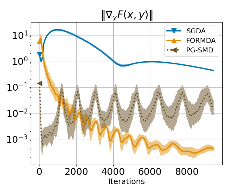
Figure 1 shows the average change in the stochastic gradient norm and the distance from the iteration point to the optimal value point for 5 independent runs of the four test algorithms, and the shaded area around the line indicates the standard deviation. It can be found that the proposed FORMDA algorithm is better than SGDA and close to the performance of PG-SMD.

Secondly, we consider a robust learning problem over multiple domains Qian . Let $P_{1},\ldots,P_{M}$ denote $M$ distributions of data. Robust learning over multiple domains is to minimize the maximum of the expected losses over the $M$ distributions, it can be formulated as the following stochastic nonconvex-concave minimax problem:

\min_{x\in\mathcal{X}}\max_{m}\mathbb{E}_{\zeta\sim P_{m}}[F(x\mathchar 24635\relax\;\zeta)]=\min_{x}\max_{y\in\Delta}\sum_{m=1}^{M}y_{m}f_{m}(x),

where $f_{m}(x)=\mathbb{E}_{\zeta\sim P_{m}}[F(x\mathchar 24635\relax\;\zeta)]$ , $F(x\mathchar 24635\relax\;\zeta)$ is a nonnegative loss function, $x$ denotes the network parameters, $y\in\Delta$ describes the weights over different tasks and $\Delta$ is the simplex, i.e., $\Delta=\left\{(y_{1},\cdots,y_{M})^{T}\mid\sum_{m=1}^{M}y_{m}=1,y_{m}\geq 0\right\}$ . We consider two image classification problems with MNIST and CIFAR10 datasets. Our goal is to train a neural network that works on these two completely unrelated problems simultaneously. The quality of the algorithm for solving a robust learning problem over multiple domains is measured by the worst case accuracy over all domains Qian .

We compare the numerical performance of the proposed FORMDA algorithm with SGDA algorithm Lin2019 and PG-SMD algorithm Rafique . We use cross-entropy loss as our loss function and set the batch size in all tasks to be 32. All algorithms were run for 50 epochs. The parameters in FORMDA are chosen to be $\eta_{k}=\frac{1}{(k+12)^{5/13}+1}$ , $\alpha_{k}=\frac{0.5}{(k+12)^{2/13}+1}$ , $\rho_{k}=\frac{8}{(k+11)^{2/13}+2}$ , $\gamma_{k}=\frac{3}{(k+12)^{8/13}+1}$ , $\theta_{k}=\frac{2}{(k+12)^{8/13}+1}$ , $\beta=0.001$ . All the parameters of the PG-SMD algorithm and the SGDA algorithm are chosen the same as that in Rafique and Lin2019 respectively.

Figure 2 shows the testing accuracy on MNIST and CIFAR10 datasets. It can be found that the proposed FORMDA algorithm outperforms SGDA and has similar performance to PG-SMD.

4 Conclusions

In this paper, we propose an accelerated FORMDA algorithm for solving stochastic nonconvex-concave minimax problems. The iteration complexity of the algorithm is proved to be $\tilde{\mathcal{O}}(\varepsilon^{-6.5})$ to obtain an $\varepsilon$ -stationary point. It owns the optimal complexity bounds within single-loop algorithms for solving stochastic nonconvex-concave minimax problems till now. Moreover, we can extend the analysis to the scenarios with possibly nonsmooth objective functions, and obtain that the iteration complexity is $\tilde{\mathcal{O}}(\varepsilon^{-6.5})$ . Numerical experiments show the efficiency of the proposed algorithm. Whether there is a single-loop algorithm with better complexity for solving this type of problem is still worthy of further research.

\bmhead

Acknowledgments The authors are supported by National Natural Science Foundation of China under the Grant (Nos. 12071279 and 12471294).

Declarations

•

Conflict of interest The authors have no relevant financial or non-financial interests to disclose.
•

Data availability Data sharing not applicable to this article as no datasets were generated or analyzed during the current study.

References

(1) Abadeh S S, Esfahani P M M, and Kuhn D. Distributionally robust logistic regression. In NeurIPS, 2015: 1576-1584.
(2) Arjovsky M, Chintala S, Bottou L. Wasserstein generative adversarial networks. International conference on machine learning. PMLR, 2017: 214-223.
(3) Bertsekas D P. Nonlinear programming. Journal of the Operational Research Society, 1997, 48(3): 334-334.
(4) Boroun M, Alizadeh Z, Jalilzadeh A. Accelerated primal-dual scheme for a class of stochastic nonconvex-concave saddle point problems. arXiv preprint arXiv:2303.00211, 2023.
(5) Bot R I, Böhm A. Alternating proximal-gradient steps for (stochastic) nonconvex-concave minimax problem. SIAM Journal on Optimization, 2023, 33(3): 1884-1913.
(6) Böhm A. Solving nonconvex-nonconcave min-max problems exhibiting weak minty solutions. arXiv preprint arXiv:2201.12247, 2022.
(7) Chen Y, Lan G, Ouyang Y. Accelerated schemes for a class of variational inequalities. Mathematical Programming,2017,165(1):113-149.
(8) Cai Y, Oikonomou A, Zheng W. Accelerated algorithms for monotone inclusions and constrained nonconvex-nonconcave min-max optimization. arXiv preprint arXiv:2206.05248, 2022.
(9) Chen J, Lau V K N. Convergence analysis of saddle point problems in time varying wireless systems—Control theoretical approach. IEEE Transactions on Signal Processing, 2011, 60(1): 443-452.
(10) Diakonikolas J, Daskalakis C, Jordan M. Efficient methods for structured nonconvex-nonconcave min-max optimization. International Conference on Artificial Intelligence and Statistics. PMLR, 2021: 2746-2754.
(11) Doan T. Convergence rates of two-time-scale gradient descent-ascent dynamics for solving nonconvex min-max problems. Learning for Dynamics and Control Conference, PMLR, 2022:192-206.
(12) Grimmer B, Lu H, Worah P, Mirrokni V. The landscape of the proximal point method for nonconvex-nonconcave minimax optimization.Mathematical Programming, 2023, 201(1-2): 373-407.
(13) Giannakis G B, Ling Q, Mateos G, Schizas I D, and Zhu H. Decentralized learning for wireless communications and networking. Splitting Methods in Communication, Imaging, Science, and Engineering, Springer, Cham, 2016:461-497.
(14) Giordano R, Broderick T andJordan M I. Covariances, robustness, and variational bayes. Journal of Machine Learning Research, 19(51), 2018.
(15) Huang F, Gao S, Pei J, Huang H. Accelerated zeroth-order and first-order momentum methods from mini to minimax optimization. Journal of Machine Learning Research, 2022, 23: 1-70.
(16) Huang F. Enhanced Adaptive Gradient Algorithms for Nonconvex-PL Minimax Optimization. arXiv preprint arXiv:2303.03984, 2023.
(17) Hamedani E Y, Aybat N S. A primal-dual algorithm with line search for general convex-concave saddle point problems. SIAM Journal on Optimization, 2021, 31(2): 1299-1329.
(18) Hajizadeh S, Lu H, Grimmer B. On the linear convergence of extra-gradient methods for nonconvex-nonconcave minimax problems. INFORMS Journal on Optimization, 2023.
(19) Jiang J, Chen X. Optimality conditions for nonsmooth nonconvex-nonconcave min-max problems and generative adversarial networks. arXiv preprint arXiv:2203.10914, 2022.
(20) Kong W, Monteiro R D C. An accelerated inexact proximal point method for solving nonconvex-concave min-max problems. SIAM Journal on Optimization, 2021, 31(4): 2558-2585.
(21) Kingma D P, Ba J. Adam: A method for stochastic optimization. arXiv preprint arXiv:1412.6980, 2014.
(22) Lan G, Monteiro R D C. Iteration-complexity of first-order augmented lagrangian methods for convex programming. Mathematical Programming, 2016,155(1-2):511-547.
(23) Lin T, Jin C, Jordan M. Near-optimal algorithms for minimax optimization. Conference on Learning Theory, PMLR, 2020:2738-2779.
(24) Lin H, Mairal J, Harchaoui Z. Catalyst acceleration for first-order convex optimization: from theory to practice. Journal of Machine Learning Research, 2018, 18(212): 1-54.
(25) Liao W, Hong M, Farmanbar H, and Luo Z Q. Semi-asynchronous routing for large scale hierarchical networks. In Proceedings of IEEE International Conference on Acoustics, Speech and Signal Processing (ICASSP), 2015:2894-2898.
(26) Luo L, Ye H S, Huang Z C, Zhang T. Stochastic recursive gradient descent ascent for stochastic nonconvex-strongly-concave minimax problems. NeurIPS, 2020, 33: 20566-20577.
(27) Liu S, Lu S, Chen X, et al. Min-max optimization without gradients: Convergence and applications to adversarial ml. arXiv preprint arXiv:1909.13806, 2019.
(28) Lin T, Jin C, Jordan M. On gradient descent ascent for nonconvex-concave minimax problems. International Conference on Machine Learning, PMLR, 2020:6083-6093.
(29) Lu S, Tsaknakis I, Hong M, Chen Y. Hybrid block successive approximation for one-sided nonconvex min-max problems: algorithms and applications. IEEE Transactions on Signal Processing, 2020,68:3676-3691.
(30) Lee S, Kim D. Fast extra gradient methods for smooth structured nonconvex-nonconcave minimax problems. Advances in Neural Information Processing Systems, 2021, 34:22588-22600.
(31) Mokhtari A, Ozdaglar A, Pattathil S. A unified analysis of extra-gradient and optimistic gradient methods for saddle point problems: Proximal point approach. International Conference on Artificial Intelligence and Statistics. PMLR, 2020: 1497-1507.
(32) Mateos G, Bazerque J A, and Giannakis G B. Distributed sparse linear regression. IEEE Transactions on Signal Processing, 2010, 58(10):5262-5276.
(33) Nouiehed M, Sanjabi M, Huang T, Lee J. D. Solving a class of non-convex min-max games using iterative first order methods. Advances in Neural Information Processing Systems, 2019: 14934-14942.
(34) Nemirovski A. Prox-method with rate of convergence O (1/t) for variational inequalities with Lipschitz continuous monotone operators and smooth convex-concave saddle point problems. SIAM Journal on Optimization, 2004, 15(1): 229-251.
(35) Nesterov Y. Smooth minimization of non-smooth functions. Mathematical programming, 2005, 103: 127-152.
(36) Nesterov Y. Dual extrapolation and its applications to solving variational inequalities and related problems. Mathematical Programming, 2007, 109(2): 319-344.
(37) Ouyang Y, Chen Y, Lan G, Pasiliao Jr E. An accelerated linearized alternating direction method of multipliers. SIAMJournal on Imaging Sciences, 2015, 8(1):644-681.
(38) Ouyang Y, Xu Y. Lower complexity bounds of first-order methods for convex-concave bilinear saddle-point problems.Mathematical Programming, 2021, 185(1): 1-35.
(39) Ostrovskii D, Lowy A, Razaviyayn M. Efficient search of first-order nash equilibria in nonconvex-concave smooth min-max problems. SIAM Journal on Optimization, 2021, 31(4): 2508-2538.
(40) Pan W, Shen J, Xu Z. An efficient algorithm for nonconvex-linear minimax optimization problem and its application in solving weighted maximin dispersion problem. Computational Optimization and Applications, 2021,78(1): 287-306.
(41) Qian Q, Zhu S, Tang J, Jin R, Sun B, Li H. Robust optimization over multiple domains. Proceedings of the AAAI Conference on Artificial Intelligence, 2019,33(01):4739–4746.
(42) Rafique H, Liu M, Lin Q, et al. Weakly-convex-concave min-max optimization: provable algorithms and applications in machine learning. Optimization Methods and Software, 2022, 37(3): 1087-1121.
(43) Sanjabi M, Razaviyayn M, Lee J D. Solving non-convex non-concave min-max games under polyak-Łojasiewicz condition. arXiv preprint arXiv:1812.02878, 2018.
(44) Song C, Zhou Z, Zhou Y, Jiang Y, Ma Y. Optimistic dual extrapolation for coherent non-monotone variational inequalities. Advances in Neural Information Processing Systems, 2020,33: 14303-14314.
(45) Shen J, Wang Z, Xu Z. Zeroth-order single-loop algorithms for nonconvex-linear minimax problems. Journal of Global Optimization, doi:10.1007/s10898-022-01169-5, 2022.
(46) Thekumparampil K K, Jain P, Netrapalli P,Oh S. Efficient algorithms for smooth minimax optimization. Advances inNeural Information Processing Systems, 2019:12680-12691.
(47) Tominin V, Tominin Y, Borodich E, Kovalev D, Gasnikov A, Dvurechensky P. On accelerated methods for saddle-pointproblems with composite structure. COMPUTER,2023, 15(2): 433-467.
(48) Tieleman T, Hinton G, et al. Lecture 6.5-rmsprop: Divide the gradient by a running average of its recent magnitude. COURSERA: Neural networks for machine learning, 2012, 4(2):26-31.
(49) Wang Z, Balasubramanian K, Ma S, Razaviyayn M. Zeroth-order algorithms for nonconvex minimax problems with improved complexities. arXiv preprint arXiv:2001.07819, 2020.
(50) Xu Z, Zhang H, Xu Y, Lan G. A unified single-loop alternating gradient projection algorithm for nonconvex-concave and convex-nonconcave minimax problems. Mathematical Programming, 2023, 201:635-706.
(51) Xu T, Wang Z, Liang Y, Poor H V. Gradient free minimax optimization: Variance reduction and faster convergence. arXiv preprint arXiv:2006.09361, 2020.
(52) Xu Z, Wang Z, Shen J, Dai Y. H. Derivative-free alternating projection algorithms for general nonconvex-concave minimax problems. SIAM Journal on Optimization, 34(2):1879-1908, (2024).
(53) Xu Z, Wang Z Q, Wang J L, Dai Y. H. Zeroth-order alternating gradient descent ascent algorithms for a class of nonconvex-nonconcave minimax problems. Journal of Machine Learning Research, 24(313): 1-25, (2023).
(54) Yang J, Kiyavash N, He N. Global convergence and variance-reduced optimization for a class of nonconvex-nonconcaveminimax problems.Advances in Neural Information Processing Systems, 2020, 33: 1153-1165.
(55) Yang J, Orvieto A, Lucchi A, et al. Faster single-loop algorithms for minimax optimization without strong concavity. International Conference on Artificial Intelligence and Statistics. PMLR, 2022: 5485-5517.
(56) Zhang J, Xiao P, Sun R, Luo Z. A single-loop smoothed gradient descent-ascent algorithm for nonconvex-concave min-max problems. Advances in Neural Information Processing Systems, 2020, 33:7377-7389.
(57) Zhang G, Wang Y, Lessard L, Grosse R B. Near-optimal local convergence of alternating gradient descent-ascent forminimax optimization. International Conference on Artificial Intelligence and Statistics, PMLR, 2022:7659-7679.
(58) Zhang X, Aybat N S, Gurbuzbalaban M. Sapd+: An accelerated stochastic method for nonconvex-concave minimax problems. Advances in Neural Information Processing Systems, 2022, 35: 21668-21681.

	$\displaystyle\\|\nabla_{x}G(x_{1},y,\zeta)-\nabla_{x}G(x_{2},y,\zeta)\\|$	$\displaystyle\leq l\\|x_{1}-x_{2}\\|,$
	$\displaystyle\\|\nabla_{x}G(x,y_{1},\zeta)-\nabla_{x}G(x,y_{2},\zeta)\\|$	$\displaystyle\leq l\\|y_{1}-y_{2}\\|,$
	$\displaystyle\\|\nabla_{y}G(x,y_{1},\zeta)-\nabla_{y}G(x,y_{2},\zeta)\\|$	$\displaystyle\leq l\\|y_{1}-y_{2}\\|,$
	$\displaystyle\\|\nabla_{y}G(x_{1},y,\zeta)-\nabla_{y}G(x_{2},y,\zeta)\\|$	$\displaystyle\leq l\\|x_{1}-x_{2}\\|.$

	$\displaystyle\\|y_{k+1}-y_{k+1}^{*}(x_{k+1})\\|^{2}$
$\displaystyle\leq$	$\displaystyle(1-\frac{\eta_{k}\beta\rho_{k+1}}{4})\\|y_{k}-y_{k}^{*}(x_{k})\\|^{2}-\frac{3\eta_{k}}{4}\\|\tilde{y}_{k+1}-y_{k}\\|^{2}+\frac{5L^{2}\eta_{k}}{\rho_{k+1}^{3}\beta}\\|\tilde{x}_{k+1}-x_{k}\\|^{2}$
	$\displaystyle+\frac{5\eta_{k}\beta}{\rho_{k+1}}\\|\nabla_{y}g_{k}(x_{k},y_{k})-w_{k}\\|^{2}+\frac{5(\rho_{k}-\rho_{k+1})}{\rho_{k+1}^{2}\eta_{k}\beta}(\\|y_{k+1}^{}(x_{k+1})\\|^{2}-\\|y_{k}^{}(x_{k})\\|^{2}).$	(2.27)

	$\displaystyle\frac{1}{2\eta_{k}\beta}\\|y_{k+1}-y_{k}^{*}(x_{k})\\|^{2}$
$\displaystyle\leq$	$\displaystyle(\frac{1}{2\eta_{k}\beta}-\frac{\rho_{k}}{4})\\|y_{k}-y_{k}^{*}(x_{k})\\|^{2}+(\frac{\eta_{k}}{2\beta}+\frac{\rho_{k}}{4}+\frac{L}{2}-\frac{1}{\beta})\\|\tilde{y}_{k+1}-y_{k}\\|^{2}$
	$\displaystyle+\frac{2}{\rho_{k}}\\|\nabla_{y}g_{k}(x_{k},y_{k})-w_{k}\\|^{2}.$	(2.35)

	$\displaystyle\\|y_{k+1}-y_{k+1}^{*}(x_{k+1})\\|^{2}$
$\displaystyle=$	$\displaystyle\\|y_{k+1}-y_{k}^{}(x_{k})\\|^{2}+2\langle y_{k+1}-y_{k}^{}(x_{k}),y_{k}^{}(x_{k})-y_{k+1}^{}(x_{k+1})\rangle+\\|y_{k}^{}(x_{k})-y_{k+1}^{}(x_{k+1})\\|^{2}$
$\displaystyle\leq$	$\displaystyle(1+\frac{\eta_{k}\beta\rho_{k}}{4})\\|y_{k+1}-y_{k}^{}(x_{k})\\|^{2}+(1+\frac{4}{\eta_{k}\beta\rho_{k}})\\|y_{k}^{}(x_{k})-y_{k+1}^{*}(x_{k+1})\\|^{2}$
$\displaystyle\leq$	$\displaystyle(1+\frac{\eta_{k}\beta\rho_{k}}{4})\\|y_{k+1}-y_{k}^{*}(x_{k})\\|^{2}+(1+\frac{4}{\eta_{k}\beta\rho_{k}})\frac{\eta_{k}^{2}L^{2}}{\rho_{k+1}^{2}}\\|\tilde{x}_{k+1}-x_{k}\\|^{2}$
	$\displaystyle+(1+\frac{4}{\eta_{k}\beta\rho_{k}})\frac{\rho_{k}-\rho_{k+1}}{\rho_{k+1}}(\\|y_{k+1}^{}(x_{k+1})\\|^{2}-\\|y_{k}^{}(x_{k})\\|^{2}).$	(2.37)

	$\displaystyle\\|y_{k+1}-y_{k+1}^{*}(x_{k+1})\\|^{2}$
$\displaystyle\leq$	$\displaystyle(1-\frac{\eta_{k}\beta\rho_{k}}{2})(1+\frac{\eta_{k}\beta\rho_{k}}{4})\\|y_{k}-y_{k}^{*}(x_{k})\\|^{2}-\frac{3\eta_{k}}{4}(1+\frac{\eta_{k}\beta\rho_{k}}{4})\\|\tilde{y}_{k+1}-y_{k}\\|^{2}$
	$\displaystyle+(1+\frac{4}{\eta_{k}\beta\rho_{k}})\frac{\eta_{k}^{2}L^{2}}{\rho_{k+1}^{2}}\\|\tilde{x}_{k+1}-x_{k}\\|^{2}+\frac{4\eta_{k}\beta}{\rho_{k}}(1+\frac{\eta_{k}\beta\rho_{k}}{4})\\|\nabla_{y}g_{k}(x_{k},y_{k})-w_{k}\\|^{2}$
	$\displaystyle+(1+\frac{4}{\eta_{k}\beta\rho_{k}})\frac{\rho_{k}-\rho_{k+1}}{\rho_{k+1}}(\\|y_{k+1}^{}(x_{k+1})\\|^{2}-\\|y_{k}^{}(x_{k})\\|^{2}).$	(2.38)