Amplitude-Phase Recombination: Rethinking Robustness of Convolutional Neural Networks in Frequency Domain
Abstract
Recently, the generalization behavior of Convolutional Neural Networks (CNN) is gradually transparent through explanation techniques with the frequency components decomposition. However, the importance of the phase spectrum of the image for a robust vision system is still ignored. In this paper, we notice that the CNN tends to converge at the local optimum which is closely related to the high-frequency components of the training images, while the amplitude spectrum is easily disturbed such as noises or common corruptions. In contrast, more empirical studies found that humans rely on more phase components to achieve robust recognition. This observation leads to more explanations of the CNN’s generalization behaviors in both robustness to common perturbations and out-of-distribution detection, and motivates a new perspective on data augmentation designed by re-combing the phase spectrum of the current image and the amplitude spectrum of the distracter image. That is, the generated samples force the CNN to pay more attention to the structured information from phase components and keep robust to the variation of the amplitude. Experiments on several image datasets indicate that the proposed method achieves state-of-the-art performances on multiple generalizations and calibration tasks, including adaptability for common corruptions and surface variations, out-of-distribution detection, and adversarial attack. The code is released on github/iCGY96/APR.
1 Introduction
In the past few years, deep learning has achieved even surpassed human-level performances in many image recognition/classification tasks [16]. However, the unintuitive generalization behaviors of neural networks, such as the vulnerability towards adversarial examples [12], common corruptions [21], the overconfidence for out-of-distribution (OOD) [20, 24, 41, 3, 2], are still confused in the community. It also leads that current deep learning models depend on the ability of training data to faithfully represent the data encountered during deployment.

To explain the generalization behaviors of neural networks, many theoretical breakthroughs have been made progressively by different model or algorithm perspectives [52, 42, 44]. Several works [49, 26] investigate the generalization behaviors of Convolutional Neural Network (CNN) from a data perspective in the frequency domain, and demonstrate that CNN benefits from the high-frequency image components which are not perceivable to humans. Furthermore, a quantitative study is provided in Figure 4 to indicate that the predictions of CNN are more sensitive to the variation of the amplitude spectrum. The above phenomena indicate that CNN tends to converge at the local optimum which is closely related to the high-frequency components of the training images. Although it is helpful when the test and training samples come from the identical distribution, yet the robustness of the CNN will be affected due of the amplitude spectrum is easily disturbed such as noises or common corruptions. On the other hand, earlier empirical studies [34, 11, 14, 30] indicate that humans rely on more the components related to the phase to recognize an object. As is known, the human eye is much more robust than CNN, and this fact encourages us to rethink the influence of amplitude and phase on CNN’s generalizability. A visualized example is shown in Figure 2 to validate the importance of phase spectrum in [34] to explain one counter-intuitive behavior of CNN. By replacing the amplitude spectrum of one Revolver with the amplitude spectrum of one Jigsaw Puzzle, the CNN classifies the fused image as Jigsaw Puzzle while humans could still recognize it as Revolver. In this example, the prediction outcomes of CNN are almost entirely determined by the amplitude spectrum of the image, which is barely perceivable to humans. On the other hand, even if the amplitude spectrum is replaced, the human is able to correctly recognize the identical object in the original picture. Moreover, we found that this phenomenon not only exists in training data (in-distribution) but also in OOD data as shown in Figure 3. In these images, after exchanging the amplitude spectrum, the prediction of CNN is also transformed with the label of the amplitude spectrum. However, humans could still observe the object structure of the original images in the converted images.
Motivated by the powerful generalizability of the human, we argue that a robust CNN should be insensitive to the change of amplitude and pay more attention to the phase spectrum. To achieve this goal, a novel data augmentation method, called Amplitude-Phase Recombination (APR), is proposed. The core of APR is to re-combine the phase spectrum of the current image and the amplitude spectrum of the distracter image to generate a new training sample, whose label is set to the current image. That is, the generated samples force the CNN to capture more structured information from phase components rather than amplitude. Specifically, the distracter image of the current image comes in two ways: other images and its augmentations generated by existing data augmentation methods such as rotate and random crop, namely APR for the pair images (APR-P) and APR for the single image (APR-S) respectively.
Extensive experiments on multiple generalizations and calibration tasks, including adaptability for common corruptions and surface variations, OOD detection, and adversarial attack, demonstrate the proposed APR outperforms the baselines by a large margin. Meanwhile, it provides a uniform explanation to the texture bias hypothesis [10] and the behaviors of both robustness to common perturbations and the overconfidence of OOD by the CNN’s over-dependence on the amplitude spectrum. That is, the various common perturbations change the high-frequency amplitude components significantly, while has little influence on the components related to the phase spectrum. Hence, the attack sample could confuse the CNN but is easily recognized by humans. On the other hand, the OOD samples often exhibit totally different image structures but may share some similarities in the high-frequency amplitude components, which makes the CNN hard to distinguish.

Our main contributions are summarized as follows: 1) We propose that a robust CNN should be robust to the amplitude variance and pay more attention to the components related to the phase spectrum by a series of quantitative and qualitative analysis, 2) a novel data augmentation method APR is proposed to force the CNN pay more attention to the phase spectrum and achieves state-of-the-art performances on multiple generalizations and calibration tasks, including adaptability for common corruptions and surface variations, OOD detection, and adversarial attack, and 3) a unified explanation is provided to the behaviors of both robustness to common perturbations and the overconfidence of OOD by the CNN’s over-dependence on the amplitude spectrum.


2 Related Work
Frequency-Based Explanation for CNN. Recently, several works provide new insights into neural network behaviors from the aspects of the frequency domain. [49] shows that high-frequency components play significant roles in promoting CNN’s accuracy, unlike human beings. Based on this observation, [49] concludes that smoothing the CNN kernels helps to enforce the model to use features of low frequencies. [13] proposes an adversarial attack only targeting the low-frequency components in an image, which shows that the model does utilize the features in the low-frequency domains for predictions instead of only learning from high-frequency components. [45] demonstrates that state-of-the-art defenses are nearly as vulnerable as undefended models under low-frequency perturbations, which implies current defense techniques are only valid against adversarial attacks in the high-frequency domain. On the other side, [32] demonstrates that CNNs can capture extra implicit features of the phase spectrum which are beneficial to face forgery detection. However, there are not works to give a qualitative study of the roles of amplitude and phase spectrums for the generalization behavior of CNN.
Data Augmentation. Data augmentation has been widely used to prevent deep neural networks from over-fitting to the training data [1], and greatly improve generalization performance. The majority of conventional augmentation methods generate new data by applying transformations depending on the data type or the target task [6]. [55] proposes mixup, which linearly interpolates between two input data and utilizes the mixed data with the corresponding soft label for training. Then, CutMix [53] suggests a spatial copy and paste based mixup strategy on images. AutoAugment [6] is a learned augmentation method, where a group of augmentations is tuned to optimize performance on a downstream task. AugMix [21] helps models withstand unforeseen corruptions by simply mixing random augmentations. However, many methods substantially degrade accuracy on non-adversarial images [36] or need adaptive and complex parameters to different tasks.
3 The Secret of CNN in the Frequency Domain
3.1 Qualitative Study on the Frequency Domain
Beyond the examples in Figure 2 and 3, here more qualitative analyses are given to measure the contributions of amplitude and phase. Several experiments are conducted on CIFAR-10 [28] to evaluate the performances of the CNNs which are trained with the inversed images by various types of amplitude and phase spectra. For the image , its frequency domain is composed by amplitude and phase as:
| (1) |
where indicates the element-wise multiplication of two matrices. Here, four types of amplitude spectra, , , , and are combined with four types of amplitude spectra, including , , , and , respectively. Here , , and , , represent the amplitude spectrum and phase of low-frequency, intermediate-frequency and high-frequency by low-pass , high-pass , and band-pass filters, respectively. Noted in Eq.(1), if one element of is zero, then the corresponding element of would be zero, and the phase spectrum is not able to be considered. To alleviate the influence of this, we define the transfer function as:
Finally, , , , and are combined with , , , and , respectively.

For quantitative evaluation, we trained the ResNet-18 with the inversed images by the above each pair of amplitude and phase spectra:
| (2) |
where is the inverse Discrete Fourier Transform (DFT), and means the CNN model with the learnable parameters .
The test accuracies of the model trained by each pair are shown in Figure 4. It is clear that the combination of phase and amplitude in the corresponding frequency domain achieves better performance in their various combinations, which indicates the CNN can capture effective information from both amplitude and phase spectrum. Moreover, when fixing the amplitude spectrum and phase spectrum respectively, the range of change without amplitude is larger than the case without phase according to the two directions of the arrow. It indicates that the convergence of the CNN more relies on the amplitude spectrum and neglects the phase spectrum.
Furthermore, we randomly select samples from CIFAR-10. Firstly, we generate 1000 corrupted samples by Gaussian noise and show the distribution of corrupted samples and original samples as shown in Figure 5(a). We could observe the amplitude spectrum in high-frequency of two types of samples is so different while the corrupted sample is just added invisible noise. Hence, CNN would make the wrong prediction when the amplitude spectrum is changed. This is also consistent with the conclusion that CNN captured high-frequency information in [49]. Therefore, we propose an assumption (referred to as A1) that presumes:
Assumption 1.
CNN without effective training restrictions tends to perceive more amplitude spectrum instead of the phase spectrum.
Then, we can formulate another formal statement for the robustness of CNN as:
Corollary 1.
With the assumption A1, there exists a sample with its amplitude and phase , that the model without effective training restrictions cannot predict robustly for where is the upper bound of the perturbation allowed.


Secondly, we randomly select OOD samples from CIFAR-100. As shown in Figure 5(b), it is not able to distinguish the amplitude spectrum in high-frequency of in-distribution and out-of-distribution, even these samples are from different categories. As a result, CNN would be overconfident for some distributions when similar amplitude information appears. Therefore, we first attempt to provide an assumption (referred to as A2) for the behaviors of the robustness to common perturbations and the overconfidence of OOD:
Assumption 2.
The behaviors of the sensitivity to common perturbations and the overconfidence of OOD may be all due to CNN’s over-dependence on the amplitude spectrum.
Meanwhile, we can extend our main argument for OOD to a new formal statement:
Corollary 2.
With the assumptions A1 and A2, there exists a in-distribution sample and an out-of-distribution sample with their amplitude and phase , that the model without effective training restrictions would give a high confidence of the for .
The proof is a direct outcome of the previous discussion and thus omitted. The Corollary 1 has been proved in previous works [49, 42, 44] and Corollary 2 can also be verified empirically (e.g., in Figure 2 and 3), therefore we can safely state that these two corollaries can serve as the alternative explanations to the generalization behavior of CNN. Meanwhile, we provide more examples for proof in Appendix.
3.2 The Role of the Phase Spectrum
Previous works [34, 11] have shown many of the important features of a signal are preserved if only the phase spectrum is retained. Meanwhile, several works of image saliency [14, 30] shown the connection of phase spectrum with the fixation of the human visual system. Further, we wish to explore why this important information of the image is retained in the phase spectrum. Here, we reinterpret the concept of discrete Fourier transforms from the perspective of template-based contrast computation [30].
Give a gray image with resolution , its complex-valued Fourier coefficient at can be computed as:
where . Then, the real and the imaginary parts of can be rewritten as:

The frequency in by Fourier transform can be interpreted as computing by four template-based contrasts:
| (3) |
Moreover, we can define templates for an image based on the signs of the real-part and the imaginary-part. A template-based example is shown in Figure 6. More examples for templates are shown in Appendix.
Meanwhile, the phase spectrum for the image is equal to , which can be reinterpreted as:
| (4) |
In Eq.(4), first, we can observe that the above four templates are encoded in the spectral phase. Hence, all templates are contained in the phase spectrum. This template-based contrast can help to explain the importance of the phase spectrum. Once the templates containing more targets without distractors are correctly estimated, the model can highly effectively locate the target objects [30]. On the other hand, these templates in the phase spectrum could help to recover the structural information of the original image even without the original amplitude spectrum as shown in Figure 3. The robustness human visual system can also rely on this visible structured information for recognition.

4 Amplitude-Phase Recombination
Motivated by the powerful generalizability of the human, we argue that reducing the dependence on the amplitude spectrum and enhancing the ability to capture phase spectrum can improve the robustness of CNN. Therefore, we introduce a none-parameter data augmentation routine, termed as Amplitude-Phase Recombination (APR), constructing more effective training examples based on the single sample or pair samples.
| Standard | Cutout | Mixup | CutMix | Adv Training | APR-P | AutoAugment | AugMix | APR-S | ARP-SP | ||
| CIFAR-10-C | AllConvNet | 30.8 | 32.9 | 24.6 | 31.3 | 28.1 | 21.5 | 29.2 | 15.0 | 14.8 | 11.5 |
| DenseNet | 30.7 | 32.1 | 24.6 | 33.5 | 27.6 | 20.3 | 26.6 | 12.7 | 12.3 | 10.3 | |
| WideResNet | 26.9 | 26.8 | 22.3 | 27.1 | 26.2 | 18.3 | 23.9 | 11.2 | 10.6 | 9.1 | |
| ResNeXt | 27.5 | 28.9 | 22.6 | 29.5 | 27 | 18.5 | 24.2 | 10.9 | 11.0 | 9.1 | |
| Mean | 29.0 | 30.2 | 23.5 | 30.3 | 27.2 | 19.7 | 26 | 12.5 | 12.2 | 10.0 | |
| CIFAR-100-C | AllConvNet | 56.4 | 56.8 | 53.4 | 56.0 | 56.0 | 47.5 | 55.1 | 42.7 | 39.8 | 35.9 |
| DenseNet | 59.3 | 59.6 | 55.4 | 59.2 | 55.2 | 49.8 | 53.9 | 39.6 | 38.3 | 35.8 | |
| WideResNet | 53.3 | 53.5 | 50.4 | 52.9 | 55.1 | 44.7 | 49.6 | 35.9 | 35.5 | 32.9 | |
| ResNeXt | 53.4 | 54.6 | 51.4 | 54.1 | 54.4 | 44.2 | 51.3 | 34.9 | 33.7 | 31.0 | |
| Mean | 55.6 | 56.1 | 52.6 | 55.5 | 55.2 | 46.6 | 52.5 | 38.3 | 36.8 | 33.9 | |
APR for the Pair Samples (APR-P). Firstly, and are two examples drawn at random from our training data. The main principle of APR is to change the amplitude spectrum as much as possible while keeping the phase spectrum and the corresponding labels unchanged. Hence, the APR-P could be defined as:
| (5) |
Then, the inversed training pair samples and are generated. Note that we use labels of phase as targets to allow the model to find the effective structured information in the phase spectrum. Meanwhile, through a variety of spectrum changes, the model gradually ignores the information from the imperceptible amplitude spectrum. It can be implemented by the way as Mixup [15] that uses a single data loader to obtain one minibatch, and then APR-P is applied to the original minibatch and the minibatch after random shuffling.
APR for the Single Sample (APR-S). For a single training sample, we consider a set consisting of different (random or deterministic) transformations, denoted . Here, we attempt to consider that the sample and its transformed sample are two different samples with the same label. The process of APR-S could be denoted as:
| (6) |
where and are transformations set based on different random seeds or sequences.
Moreover, these two ways of amplitude-phase recombination could be used in combination and generate different gains for different data. Several examples from APR-P and APR-S are shown in Figure 7.
5 Experiments
Datasets. CIFAR-10 and CIFAR-100 [28] datasets contain small xx color natural images, both with 50,000 training images and 10,000 testing images. CIFAR-10 has 10 categories, and CIFAR-100 has 100. The larger and more difficult ImageNet [7] dataset contains 1,000 classes of approximately 1.2 milion large-scale color images.
In order to measure a model’s resilience to common corruptions and surface variations, we evaluate methods on the CIFAR-10-C, CIFAR-100-C, and ImageNet-C datasets [18]. These datasets are constructed by corrupting the original CIFAR and ImageNet testsets. For each dataset, there are a total of 15 noise, blur, weather, and digital corruption types, each appearing at 5 severity levels or intensities. Since these datasets are used to measure network behavior under data shift, these 15 corruptions are not introduced into the training procedure.
To measure the ability for OOD detection, we consider CIFAR-10 as in-distribution and the following datasets as OOD: SVHN [33], resized LSUN and ImageNet [31], CIFAR-100 [28].
| Method | Test acc. | CIFAR-10 | Mean | |||||
|---|---|---|---|---|---|---|---|---|
| SVHN | LSUN | ImageNet | LSUN(FIX) | ImageNet(FIX) | CIFAR100 | |||
| Cross Entropy (CE) | 93.0 | 88.6 | 90.7 | 88.3 | 87.5 | 87.4 | 85.8 | 88.1 |
| CE w/ Cutout [8] | 95.8 | 93.6 | 94.5 | 90.2 | 92.2 | 89.0 | 86.4 | 91.0 |
| CE w/ Mixup [15] | 96.1 | 78.1 | 80.7 | 76.5 | 80.7 | 76.0 | 74.9 | 77.8 |
| CE w/ APR-P | 95.0 | 98.1 | 93.7 | 95.2 | 91.4 | 91.1 | 88.9 | 93.1 |
| SupCLR [27] | 93.8 | 97.3 | 92.8 | 91.4 | 91.6 | 90.5 | 88.6 | 92.0 |
| CSI [47] | 94.8 | 96.5 | 96.3 | 96.2 | 92.1 | 92.4 | 90.5 | 94.0 |
| CE w/ APR-S | 95.1 | 90.4 | 96.1 | 94.2 | 90.9 | 89.1 | 86.8 | 91.3 |
| CE w/ APR-SP | 95.6 | 97.7 | 97.9 | 96.3 | 93.7 | 92.8 | 89.5 | 94.7 |
5.1 CIFAR-10 and CIFAR-100
Training Setup. For a model’s resilience to common corruptions and surface variations, we adopt various architectures including an All Convolutional Network [40], a DenseNet-BC () [25], a 40-2 Wide ResNet [54], and a ResNeXt-29 (32x4) [51]. All networks use an initial learning rate of 0.1 which decay every 60 epochs. All models require 200 epochs for convergence. We optimize with stochastic gradient descent using Nesterov momentum [46]. All input images are processed with ”Standard” random left-right flipping and cropping prior to any augmentations. For the data augmentations of APR-S, we adopt those used in [21] which is shown in Appendix. For the OOD detection, we use ResNet-18 [17] with the same training strategies above. The data augmentations are set up the same as the above. We report the Area Under the Receiver Operating Characteristic curve (AUROC) [20] as a threshold-free evaluation metric for a detection score. We divide all methods into two categories, one is to add one augmentation on the basis of standard augmentations (random left-right flipping, and cropping), and the other is to add a combination of multiple augmentations as [5, 21].
Common Corruptions and Surface Variations. We first evaluate all methods with common corruptions and surface variations, such as noise, blur, weather, and digital. Compared to the Mixup or CutMix based on pair images, our APR-P with exchanging amplitude spectrum in pair images achieves 6% lower absolute corruption error for CIFAR-100 as shown in Table 1. For methods based on a combination of multiple augmentations, our APR-S of the single image with just Cross-Entropy loss (CE) performs better than AugMix with simply mixing random augmentations and using the Jensen-Shannon loss substantially. When combining our method for single and pair images, the APR-SP achieves 5% performance improvement compared with AugMix in CIFAR-100. In addition to surpassing numerous other data augmentation techniques, Table 1 also demonstrates that these gains come from simple recombination of amplitude and phase without a complex mixup strategy. More comparisons and results about test accuracy are shown in Appendix.
Out-of-Distribution Detection. We compare APR with those augmentations (Cutout, and Mixup) and those several training methods, the cross-entropy, supervised contrastive learning (SupCLR) [27], and state-of-the-art method contrasting shifted instances (CSI) [47]. Since our goal is to calibrate the confidence, the maximum softmax probability is used to detect OOD samples. Table 2 shows the results. Firstly, APR-P consistently improves 2% AUROC than Cutout on CIFAR-10 while maintaining test accuracy. Then, after combining APR based on single and pair images, APR-SP exceeds CSI and gains in almost all OOD tasks. APR promotes CNN to pay more attention to the phase spectrum so that some OOD samples that affect CNN’s decision-making in amplitude spectrum could be detected effectively.
| Method | Clean | AutoAttack[4] |
|---|---|---|
| FSGM [50] | 83.3 | 43.2 |
| FSGM w/ Cutout | 81.3 | 41.6 |
| FSGM w/ APR-P | 85.3 | 44.1 |
| FSGM w/ APR-S | 83.5 | 45.0 |
| FSGM w/ APR-SP | 84.3 | 45.7 |
Adversarial Attack. Moreover, the phenomenon of CNN focusing on amplitude spectrum leads to a question of whether APR can improve the adversarial robustness of models. Here, we evaluate several augmentations against one adversarial attack, AutoAttack [4]. Table 3 shows the AutoAttack [4] performance by combining different methods with revisiting adversarial training method of FSGM [50] on CIFAR10. The cutout is not able to effectively against adversarial attacks compared with the baseline with revisiting adversarial training method of FSGM [50]. On the contrary, APR could effectively against AutoAttack while maintaining test accuracy. Compared with APR-P, APR-S for single images achieves more improvement on AutoAttack. Furthermore, the combination of these two strategies achieves better performance. It is evident that APR-SP improves the ability of the original model not only on clean images but also against adversarial attacks.
| Method | Test Err. | Noise | Blur | Weather | Digital | mCE | |||||||||||
|---|---|---|---|---|---|---|---|---|---|---|---|---|---|---|---|---|---|
| Gauss | Shot | Impulse | Defocus | Glass | Motion | Zoom | Snow | Frost | Fog | Bright | Contrast | Elastic | Pixel | JPEG | |||
| Standard | 23.9 | 79 | 80 | 82 | 82 | 90 | 84 | 80 | 86 | 81 | 75 | 65 | 79 | 91 | 77 | 80 | 80.6 |
| Patch Uniform | 24.5 | 67 | 68 | 70 | 74 | 83 | 81 | 77 | 80 | 74 | 75 | 62 | 77 | 84 | 71 | 71 | 74.3 |
| AutoAugment(AA) | 22.8 | 69 | 68 | 72 | 77 | 83 | 80 | 81 | 79 | 75 | 64 | 56 | 70 | 88 | 57 | 71 | 72.7 |
| Random AA | 23.6 | 70 | 71 | 72 | 80 | 86 | 82 | 81 | 81 | 77 | 72 | 61 | 75 | 88 | 73 | 72 | 76.1 |
| MaxBlur pool | 23.0 | 73 | 74 | 76 | 74 | 86 | 78 | 77 | 77 | 72 | 63 | 56 | 68 | 86 | 71 | 71 | 73.4 |
| SIN | 27.2 | 69 | 70 | 70 | 77 | 84 | 76 | 82 | 74 | 75 | 69 | 65 | 69 | 80 | 64 | 77 | 73.3 |
| AugMix | 22.4 | 65 | 66 | 67 | 70 | 80 | 66 | 66 | 75 | 72 | 67 | 58 | 58 | 79 | 69 | 69 | 68.4 |
| APR-S | 24.5 | 61 | 64 | 60 | 73 | 87 | 72 | 81 | 72 | 67 | 62 | 56 | 70 | 83 | 79 | 71 | 70.5 |
| APR-P | 24.4 | 64 | 68 | 68 | 70 | 89 | 69 | 81 | 69 | 69 | 55 | 57 | 58 | 85 | 66 | 72 | 69.3 |
| APR-SP | 24.4 | 55 | 61 | 54 | 68 | 84 | 68 | 80 | 62 | 62 | 49 | 53 | 57 | 83 | 70 | 69 | 65.0 |
| DeepAugment [19] | 26.3 | 49 | 49 | 48 | 62 | 74 | 68 | 79 | 68 | 64 | 64 | 57 | 63 | 78 | 50 | 73 | 63.1 |
| DeepAugment+APR-SP | 26.4 | 44 | 45 | 41 | 57 | 70 | 60 | 79 | 56 | 56 | 50 | 54 | 54 | 78 | 47 | 71 | 57.5 |
5.2 ImageNet Classsification
Training Setup. ResNet-50 [17] is trained with an initial learning rate of 0.1 which decay every 30 epochs. It is optimized with stochastic gradient descent using momentum [35], and requires 100 epochs for convergence. All input images are pre-processed with standard random cropping horizontal mirroring. For the data augmentations of APR-S, we adopt those used in [21] without augmentations such as contrast, color, brightness, sharpness, and Cutout, which may overlap with the corruptions of ImageNet-C. Following [21], we utilize the convention of normalizing the corruption error by the corruption err of AlexNet [29]. Corruption Error () is computed as . The average of the 15 corruption errors is as the Mean Corruption Error ().


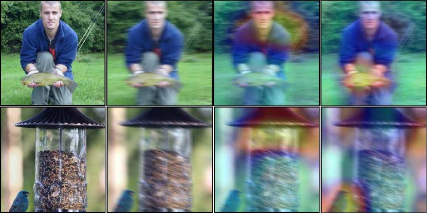
Results. Our method APR-SP achieves 15% improvement than the baseline while maintaining test accuracy. Other methods such as AutoAugment and AugMix require a more complex combination strategy, while ours does not. Meanwhile, APR improves corruption robustness [21] and uncertainty estimates across almost every individual corruption and severity level while the performance of zoom blur is comparable with most methods. APR-SP gets about 5% improvement than APR-S and APR-P, and APR-SP with DeepAugment improves 6% than the reproduced DeepAugment [19]. As shown in Figure 8, the CNN trained with APR-SP is able to focus on the parts of the target object for classification even in a heavy fog. These results demonstrate that scaling up APR from CIFAR to ImageNet also leads to state-of-the-art results in robustness and uncertainty estimation.
5.3 Labeled by Amplitude or Phase?
For our proposed APR-P, we utilize the labels of phase spectrum in the pair samples. Naturally, we wish to explore the impact of using labels amplitude and phase separately. Here, we add a linear classifier layer in ResNet-18 to predict the labels of the amplitude spectrum. The model is trained for the sample combined by the phase spectrum and the amplitude spectrum by optimizing:
| (7) |
Then, the final prediction is defined as . The recognition ability of the model to different distribution changes with as shown in Figure 9. With the enhancement of the weight of phase prediction, the accuracy of the model is improved, especially for common corruptions and surface variations, and OOD detection. Meanwhile, the detection ability of the model for OOD samples becomes stronger with the increase of phase attention. This result could further prove the correctness of our corollaries.

6 Conclusion & Outlook
This paper proposes a series of quantitative and qualitative analyses to indicate that a robust CNN should be robust to the amplitude variance and pay more attention to the components related to the phase spectrum. Then, a novel data augmentation method APR is proposed to force the CNN to pay more attention to the phase spectrum and achieves state-of-the-art performances on multiple generalizations and calibration tasks. Also, a unified explanation is provided to the behaviors of both adversarial attack and the overconfidence of OOD by the CNN’s over-dependence on the amplitude spectrum. Looking forward, more research directions about phase could be exploited in the future era of computer vision research. One possible direction is to explore how to represent part-whole hierarchies [23] in neural networks that rely on the phase spectrum. On the other hand, more CNN models [39, 37] or convolution operations to capture more phase information are worth exploring.
Acknowledgments. This work is partially supported by grants from the National Key R&D Program of China under Grant 2020AAA0103501, and grants from the National Natural Science Foundation of China under contract No. 61825101 and No. 62088102.
References
- [1] Chris M Bishop. Training with noise is equivalent to tikhonov regularization. Neural computation, 7(1):108–116, 1995.
- [2] Guangyao Chen, Peixi Peng, Xiangqian Wang, and Yonghong Tian. Adversarial reciprocal points learning for open set recognition. arXiv preprint arXiv:2103.00953, 2021.
- [3] Guangyao Chen, Limeng Qiao, Yemin Shi, Peixi Peng, Jia Li, Tiejun Huang, Shiliang Pu, and Yonghong Tian. Learning open set network with discriminative reciprocal points. In Proceedings of European Conference on Computer Vision, pages 507–522. Springer, 2020.
- [4] Francesco Croce and et.al. Reliable evaluation of adversarial robustness with an ensemble of diverse parameter-free attacks. In ICML, 2020.
- [5] Ekin D Cubuk, Barret Zoph, Dandelion Mane, Vijay Vasudevan, and Quoc V Le. Autoaugment: Learning augmentation policies from data. In Proceedings of the IEEE conference on computer vision and pattern recognition, 2018.
- [6] Ekin D Cubuk, Barret Zoph, Dandelion Mane, Vijay Vasudevan, and Quoc V Le. Autoaugment: Learning augmentation strategies from data. In Proceedings of the IEEE/CVF Conference on Computer Vision and Pattern Recognition, pages 113–123, 2019.
- [7] Jia Deng, Wei Dong, Richard Socher, Li-Jia Li, Kai Li, and Li Fei-Fei. Imagenet: A large-scale hierarchical image database. In 2009 IEEE conference on computer vision and pattern recognition, pages 248–255. Ieee, 2009.
- [8] Terrance DeVries and Graham W Taylor. Improved regularization of convolutional neural networks with cutout. arXiv preprint arXiv:1708.04552, 2017.
- [9] Akshay Raj Dhamija, Manuel Günther, and Terrance Boult. Reducing network agnostophobia. In Advances in Neural Information Processing Systems, pages 9157–9168, 2018.
- [10] Robert Geirhos, Patricia Rubisch, Claudio Michaelis, Matthias Bethge, Felix A Wichmann, and Wieland Brendel. Imagenet-trained cnns are biased towards texture; increasing shape bias improves accuracy and robustness. arXiv preprint arXiv:1811.12231, 2018.
- [11] Dennis C Ghiglia and Mark D Pritt. Two-dimensional phase unwrapping: theory, algorithms, and software, volume 4. Wiley New York, 1998.
- [12] Ian J Goodfellow, Jonathon Shlens, and Christian Szegedy. Explaining and harnessing adversarial examples. In International Conference on Learning Representations, 2015.
- [13] Chuan Guo, Jared S Frank, and Kilian Q Weinberger. Low frequency adversarial perturbation. In Uncertainty in Artificial Intelligence, pages 1127–1137. PMLR, 2020.
- [14] Chenlei Guo, Qi Ma, and Liming Zhang. Spatio-temporal saliency detection using phase spectrum of quaternion fourier transform. In 2008 IEEE Conference on Computer Vision and Pattern Recognition, pages 1–8. IEEE, 2008.
- [15] Hongyu Guo, Yongyi Mao, and Richong Zhang. Mixup as locally linear out-of-manifold regularization. In Proceedings of the AAAI Conference on Artificial Intelligence, volume 33, pages 3714–3722, 2019.
- [16] Kaiming He, Xiangyu Zhang, Shaoqing Ren, and Jian Sun. Delving deep into rectifiers: Surpassing human-level performance on imagenet classification. In Proceedings of the IEEE International Conference on Computer Vision, pages 1026–1034, 2015.
- [17] Kaiming He, Xiangyu Zhang, Shaoqing Ren, and Jian Sun. Deep residual learning for image recognition. In Proceedings of the IEEE conference on computer vision and pattern recognition, pages 770–778, 2016.
- [18] Dan Hendrycks and Thomas Dietterich. Benchmarking neural network robustness to common corruptions and perturbations. arXiv preprint arXiv:1903.12261, 2019.
- [19] Dan Hendrycks and et.al. The many faces of robustness: A critical analysis of out-of-distribution generalization. arXiv preprint arXiv:2006.16241, 2020.
- [20] Dan Hendrycks and Kevin Gimpel. A baseline for detecting misclassified and out-of-distribution examples in neural networks. In Proceedings of International Conference on Learning Representations, 2017.
- [21] Dan Hendrycks, Norman Mu, Ekin Dogus Cubuk, Barret Zoph, Justin Gilmer, and Balaji Lakshminarayanan. Augmix: A simple data processing method to improve robustness and uncertainty. In International Conference on Learning Representations, 2019.
- [22] Dan Hendrycks, Kevin Zhao, Steven Basart, Jacob Steinhardt, and Dawn Song. Natural adversarial examples. arXiv preprint arXiv:1907.07174, 2019.
- [23] Geoffrey Hinton. How to represent part-whole hierarchies in a neural network. arXiv preprint arXiv:2102.12627, 2021.
- [24] Yen-Chang Hsu, Yilin Shen, Hongxia Jin, and Zsolt Kira. Generalized odin: Detecting out-of-distribution image without learning from out-of-distribution data. In Proceedings of the IEEE Conference on Computer Vision and Pattern Recognition, pages 10951–10960, 2020.
- [25] Gao Huang, Zhuang Liu, Laurens Van Der Maaten, and Kilian Q Weinberger. Densely connected convolutional networks. In Proceedings of the IEEE conference on computer vision and pattern recognition, pages 4700–4708, 2017.
- [26] Andrew Ilyas, Shibani Santurkar, Logan Engstrom, Brandon Tran, and Aleksander Madry. Adversarial examples are not bugs, they are features. Advances in neural information processing systems, 32, 2019.
- [27] Prannay Khosla, Piotr Teterwak, Chen Wang, Aaron Sarna, Yonglong Tian, Phillip Isola, Aaron Maschinot, Ce Liu, and Dilip Krishnan. Supervised contrastive learning. Advances in Neural Information Processing Systems, 33, 2020.
- [28] Alex Krizhevsky, Geoffrey Hinton, et al. Learning multiple layers of features from tiny images. 2009.
- [29] Alex Krizhevsky, Ilya Sutskever, and Geoffrey E Hinton. Imagenet classification with deep convolutional neural networks. Advances in neural information processing systems, 25:1097–1105, 2012.
- [30] Jia Li, Ling-Yu Duan, Xiaowu Chen, Tiejun Huang, and Yonghong Tian. Finding the secret of image saliency in the frequency domain. IEEE transactions on pattern analysis and machine intelligence, 37(12):2428–2440, 2015.
- [31] Shiyu Liang, Yixuan Li, and R Srikant. Enhancing the reliability of out-of-distribution image detection in neural networks. In International Conference on Learning Representations, 2018.
- [32] Honggu Liu, Xiaodan Li, Wenbo Zhou, Yuefeng Chen, Yuan He, Hui Xue, Weiming Zhang, and Nenghai Yu. Spatial-phase shallow learning: Rethinking face forgery detection in frequency domain. In Proceedings of the IEEE/CVF Conference on Computer Vision and Pattern Recognition, 2021.
- [33] Yuval Netzer, Tao Wang, Adam Coates, Alessandro Bissacco, Bo Wu, and Andrew Y Ng. Reading digits in natural images with unsupervised feature learning. In Neural Information Processing Systems Workshop on Deep Learning and Unsupervised Feature Learning, 2011.
- [34] Alan V Oppenheim and Jae S Lim. The importance of phase in signals. Proceedings of the IEEE, 69(5):529–541, 1981.
- [35] Ning Qian. On the momentum term in gradient descent learning algorithms. Neural Networks, 12(1):145–151, 1999.
- [36] Aditi Raghunathan, Sang Michael Xie, Fanny Yang, John C Duchi, and Percy Liang. Adversarial training can hurt generalization. arXiv preprint arXiv:1906.06032, 2019.
- [37] Kaushik Roy, Akhilesh Jaiswal, and Priyadarshini Panda. Towards spike-based machine intelligence with neuromorphic computing. Nature, 575(7784):607–617, 2019.
- [38] Olga Russakovsky, Jia Deng, Hao Su, Jonathan Krause, Sanjeev Satheesh, Sean Ma, Zhiheng Huang, Andrej Karpathy, Aditya Khosla, Michael Bernstein, Alexander C. Berg, and Li Fei-Fei. ImageNet Large Scale Visual Recognition Challenge. International Journal of Computer Vision, 115(3):211–252, 2015.
- [39] Sara Sabour, Nicholas Frosst, and Geoffrey E Hinton. Dynamic routing between capsules. In Proceedings of the 31st International Conference on Neural Information Processing Systems, pages 3859–3869, 2017.
- [40] Tim Salimans and Diederik P Kingma. Weight normalization: a simple reparameterization to accelerate training of deep neural networks. In Proceedings of the 30th International Conference on Neural Information Processing Systems, pages 901–909, 2016.
- [41] Walter J Scheirer, Anderson de Rezende Rocha, Archana Sapkota, and Terrance E Boult. Toward open set recognition. IEEE Transactions on Pattern Analysis and Machine Intelligence, 35(7):1757–1772, 2012.
- [42] Ludwig Schmidt, Shibani Santurkar, Dimitris Tsipras, Kunal Talwar, and Aleksander Madry. Adversarially robust generalization requires more data. Advances in neural information processing systems, 31, 2018.
- [43] Ramprasaath R Selvaraju, Michael Cogswell, Abhishek Das, Ramakrishna Vedantam, Devi Parikh, and Dhruv Batra. Grad-cam: Visual explanations from deep networks via gradient-based localization. In Proceedings of the IEEE international conference on computer vision, pages 618–626, 2017.
- [44] Adi Shamir, Itay Safran, Eyal Ronen, and Orr Dunkelman. A simple explanation for the existence of adversarial examples with small hamming distance. arXiv preprint arXiv:1901.10861, 2019.
- [45] Yash Sharma, Gavin Weiguang Ding, and Marcus Brubaker. On the effectiveness of low frequency perturbations. arXiv preprint arXiv:1903.00073, 2019.
- [46] Ilya Sutskever, James Martens, George Dahl, and Geoffrey Hinton. On the importance of initialization and momentum in deep learning. In International conference on machine learning, pages 1139–1147. PMLR, 2013.
- [47] Jihoon Tack, Sangwoo Mo, Jongheon Jeong, and Jinwoo Shin. Csi: Novelty detection via contrastive learning on distributionally shifted instances. In 34th Conference on Neural Information Processing Systems (NeurIPS) 2020. Neural Information Processing Systems, 2020.
- [48] Laurens Van der Maaten and Geoffrey Hinton. Visualizing data using t-sne. Journal of machine learning research, 9(11), 2008.
- [49] Haohan Wang, Xindi Wu, Zeyi Huang, and Eric P Xing. High-frequency component helps explain the generalization of convolutional neural networks. In Proceedings of the IEEE/CVF Conference on Computer Vision and Pattern Recognition, pages 8684–8694, 2020.
- [50] Eric Wong and et.al. Fast is better than free: Revisiting adversarial training. In ICLR, 2019.
- [51] Saining Xie, Ross Girshick, Piotr Dollár, Zhuowen Tu, and Kaiming He. Aggregated residual transformations for deep neural networks. In Proceedings of the IEEE conference on computer vision and pattern recognition, pages 1492–1500, 2017.
- [52] Yang You, Igor Gitman, and Boris Ginsburg. Scaling sgd batch size to 32k for imagenet training. In Proceedings of International Conference on Learning Representations, 2017.
- [53] Sangdoo Yun, Dongyoon Han, Seong Joon Oh, Sanghyuk Chun, Junsuk Choe, and Youngjoon Yoo. Cutmix: Regularization strategy to train strong classifiers with localizable features. In Proceedings of the IEEE/CVF International Conference on Computer Vision, pages 6023–6032, 2019.
- [54] Sergey Zagoruyko and Nikos Komodakis. Wide residual networks. In British Machine Vision Conference 2016. British Machine Vision Association, 2016.
- [55] Hongyi Zhang, Moustapha Cisse, Yann N Dauphin, and David Lopez-Paz. mixup: Beyond empirical risk minimization. In International Conference on Learning Representations, 2018.
Appendix
In the supplemental material, we firstly visualize the distributions of the corrupted samples, adversarial samples, and OOD samples in the frequency domain to validate the Assumption 2 in the main text in Section A. Then, several typical templates of the phase spectrum are shown in Section B to intuitionally explain the rationality of the proposed APR method, and the implementation details of the data augmentation of APR-S are listed in Section C. In Section D, the Fourier analysis is provided to demonstrate the various gains from APR-P and APR-S, and the clean error analysis and OOD detection on ImageNet are also listed to clarify the excellent scalability of our method.


A More Studies on the Frequency Domain.
Here, we show more studies of the different types of the amplitude spectrum. For all samples in CIFAR, we generate the low-frequency, intermediate-frequency and high-frequency counterparts with for non-zero parts set to , and , respectively. In Figure 10, we show the amplitude spectrum distributions of low-frequency, intermediate-frequency, and high-frequency from original samples, their corrupted samples, adversarial samples, and OOD samples respectively.
Firstly, for corrupted samples and adversarial samples from a single category, we could observe that their amplitude spectrum in high-frequency and intermediate-frequency has different distribution with the original samples even if only invisible noises are introduced. Moreover, the amplitude spectrums in low-frequency of corrupted samples and adversarial samples are indistinguishable from the original images. It also explains that CNN captures the high-frequency image components for classification [49]. Hence, CNN would make a wrong prediction for ’similar’ images (corruption and adversarial samples) when the parts of the amplitude spectrum are changed.
Then, for the OOD samples from CIFAR-100, it is evident that any type of the amplitude spectrum of in-distribution and out-of-distribution could be not able to distinguish. CNN focusing on the amplitude spectrum has a huge risk that any OOD sample with a similar amplitude part of in-distribution samples would be classified as an in-distribution sample. Hence, CNN would be overconfident for some out-of-distributions when similar amplitude information appears.
Overall, the above analyses explain our Assumption 2 in the main text, that the counter-intuitive behaviors of the sensitivity to common perturbations and the overconfidence of OOD maybe both be related to CNN’s over-dependence on the amplitude spectrum. We do not focus on the high frequency only, because the OOD samples may come from the similarity of any amplitude part as shown in Figure 10. As a result, the focusing of some parts of the amplitude spectrum may create an invisible way to attack CNN, such as the adversarial attack and various corruptions (Corollary 1), and the amplitude attack or OOD attack (Corollary 2).
B Templates from the Phase Spectrum
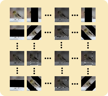


To better reveal the role of the phase spectrum, we analyze the phase spectrum in the different frequency domains. When DFT is applied on a gray image, there are totally templates which are used to compute contrast scores (as shown in Figure 11). Consequently, the frequency spectrum stores contrast values obtained at multiple scales and directions. The classification or other visual tasks could benefit from capturing the difference between targets and distractors by these templates. The templates of the lowest frequencies divide images into large regions, which are ”coarse” partitions. Then, the templates of the highest frequencies provide ”fine” partitions that achieve only high responses to noises and textures. In addition, the templates of the intermediate frequencies provide ”moderate” partitions which may include the target object, and it has also been proved that it’s beneficial for fixation prediction in [30]. These templates in the phase spectrum could help to recover the structural information of the original image even without the original amplitude spectrum [34]. The robustness human visual system can also rely on this visible structured information for recognition [34, 32].
C Augmentation Operations
The augmentation operations used in APR-S are same with [21] as shown in Figure 12. We do not use contrast, color, brightness, sharpness and Cutout as they may overlap with the corruptions of CIFAR-C and ImageNet-C.


D Additional Results

| Standard | Cutout | Mixup | CutMix | AutoAugment | Adv Training | AugMix | APR-P | APR-S | APR-SP | ||
|---|---|---|---|---|---|---|---|---|---|---|---|
| CIFAR-10-C | AllConvNet | 6.1 | 6.1 | 6.3 | 6.4 | 6.6 | 18.9 | 6.5 | 5.5 | 6.5 | 5.7 |
| DenseNet | 5.8 | 4.8 | 5.5 | 5.3 | 4.8 | 17.9 | 4.9 | 5.0 | 5.1 | 4.8 | |
| WideResNet | 5.2 | 4.4 | 4.9 | 4.6 | 4.8 | 17.1 | 4.9 | 4.8 | 5.0 | 4.3 | |
| ResNeXt | 4.3 | 4.4 | 4.2 | 3.9 | 3.8 | 15.4 | 4.2 | 4.5 | 4.5 | 3.9 | |
| Mean | 5.4 | 4.9 | 5.2 | 5.0 | 5.0 | 17.3 | 5.1 | 5.0 | 5.2 | 4.7 | |
D.1 Fourier Analysis
In order to better understand the reliance of our methods on different frequencies, here we measure the model sensitivity to the additive noise at differing frequencies. We add a total of Fourier basis vector to the CIFAR-10 test set, one at a time, and record the resulting error rate after adding each Fourier basis vector. Each point in the sensitivity heatmap shows the error rate on the CIFAR-10 test set after it has been perturbed by a single Fourier basis vector. Points corresponding to the low-frequency vectors are shown in the center of the heatmap, whereas the high-frequency vectors are farther than the center.
In Figure 13, we observe that the standard model is robust to the low-frequency perturbations but severely lacks robustness to the high-frequency perturbations, where the error rates exceed . Then, the model trained by APR-P is more robust to all frequencies, especially to the low and intermediate frequencies. Moreover, the model trained by APR-S maintains robustness to low-frequency perturbations and improves robustness to the high-frequency perturbations, but is still sensitive to the additive noise in the intermediate frequencies. This further explains the experiments in Section 5.1.2 (main text) that APR-P improves performances of both OOD detection and defense adversarial attacks tasks. From Appendix A, the adversarial samples are more different from original samples in intermediate and high frequencies, while the OOD samples may share similarities with the original samples in any frequencies. The gains of APR-P and APR-S to different frequency domains bring the gains to different tasks.
Furthermore, APR-SP (combining APR-S and APR-P) could substantially improve robustness to most frequency perturbations. The weak sensitivity to the intermediate frequencies is reasonable because of the gains for target prediction from intermediate frequencies in Appendix B.
D.2 Clean Error
Table 5 reports clean error [21] of CIFAR-10 by different methods, and the proposed method achieves the best performances on various backbone networks. APR-SP not only improves the model adaptability to the common corruptions, surface variations and OOD detection, but also improves the classification accuracy of the clean images.
| Method | AUROC | OSCR |
|---|---|---|
| Standard | 40.9 | 36.8 |
| APR-SP | 62.3 | 53.2 |
D.3 OOD Detection on ImageNet.
We conduct OOD experiments on the larger and more difficult ImageNet-1K dataset [38]. ImageNet-O [22] is adopted as the out-of-distribution dataset of ImageNet-1K. ImageNet-O includes 2K examples from ImageNet-22K [38] excluding ImageNet-1K. The ResNet 50 [17] is trained on ImageNet-1K and tested on both ImageNet-1K and ImageNet-O.
In order to evaluate the accuracy of in-distribution and the ability of OOD detection simultaneously, we introduce Open Set Classification Rate (OSCR) [9, 2] as an evaluation metric. Let is a score threshold. The Correct Classification Rate (CCR) is the fraction of the samples where the correct class has maximum probability and has a probability greater than :
| (A.1) |
where is the interest in-distribution classes that the neural network shall identify. The False Positive Rate (FPR) is the fraction of samples from OOD data that are classified as any in-distribution class with a probability greater than :
| (A.2) |
A larger value of OSCR indicates a better detection performance. As shown in Table 6, APR-SP performs better than the standard augmentations even on the large and difficult dataset. Especially, APR-SP achieves about 22% improvement on AUROC. From the OSCR, APR-SP improves the performances of the OOD detection while maintaining test accuracy. These results indicate the excellent scalability of APR in larger-scale datasets.
D.4 More CAM Visualization Examples
We also list more visualization examples with various corruptions in Figure 14 and 15, the CNN trained by APR-SP is able to focus on the target objects for classification even with different common corruptions and surface variations.