Amercing: An Intuitive, Elegant and Effective Constraint for Dynamic Time Warping

Dynamic Time Warping ($\operatorname{DTW}$) is a distance measure for time series. First developed for speech recognition [2, 3], it has been adopted across a broad spectrum of applications including gesture recognition [4], signature verification [5], shape matching [6], road surface monitoring [7], neuroscience [8] and medical diagnosis [9].

DTW sums pairwise-distances between aligned points in two series. To allow for similar events that unfold at different rates, $\operatorname{DTW}$ provides elasticity in which points are aligned. However, it is well understood that $\operatorname{DTW}$ can be too flexible in the alignments it allows. We illustrate this with respect to three series shown in Figure 1.

A natural expectation for any time series distance function $\operatorname{dist}$ is that $\operatorname{dist}(S,S)=0<\operatorname{dist}(S,T)<\operatorname{dist}(S,U)$. However, $\operatorname{DTW}(S,S)=\operatorname{DTW}(S,T)=\operatorname{DTW}(S,U)=0$. While this may be appropriate for some tasks, where all that matters is that these sequences all contain five 1s and one -1, it is inappropriate for others.

Two variants have been developed to constrain $\operatorname{DTW}$’s flexibility, Constrained $\operatorname{DTW}$ ($\operatorname{CDTW}$ [2, 3], see Section 2.2) and Weighted $\operatorname{DTW}$ ($\operatorname{WDTW}$ [10], see Section 2.3). $\operatorname{CDTW}_{w}$ constrains the alignments from warping by more than a window, $w$. Within the window, any warping is allowed, and none beyond it. Depending on $w$, there are three possibilities for how $\operatorname{CDTW}$ might assess our example:

1. 1.

   For $w\geq 2$, $\operatorname{CDTW}_{w}(S,S)=\operatorname{CDTW}_{w}(S,T)=\operatorname{CDTW}_{w}(S,U)=0$.

2. 2.

   $\operatorname{CDTW}_{1}(S,S)=\operatorname{CDTW}_{1}(S,T)=0<\operatorname{CDTW}_{1}(S,U)=8$ (see Figure 3)

3. 3.

   $\operatorname{CDTW}_{0}(S,S)=0<\operatorname{CDTW}_{0}(S,T)=\operatorname{CDTW}_{0}(S,U)$.

$\operatorname{WDTW}$ applies a multiplicative penalty to alignments that increases the more the alignment is warped. However, because the penalty is multiplicative, the perfectly matched elements in our example still lead to $\operatorname{WDTW}(S,S)=\operatorname{WDTW}(S,T)=\operatorname{WDTW}(S,U)=0$ (see Figure 4).

None of $\operatorname{DTW}$, $\operatorname{WDTW}$ or $\operatorname{CDTW}$ can be parameterized to obtain the natural expectation that $\operatorname{dist}(S,S)=0<\operatorname{dist}(S,T)<\operatorname{dist}(S,U)$.

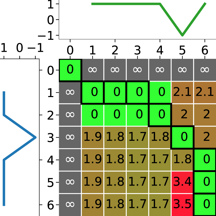
In this paper, we present Amerced DTW ($\operatorname{ADTW}$), an intuitive, elegant and effective variant of $\operatorname{DTW}$ that applies a tunable additive penalty $\omega$ for warping an alignment. To align the $-1$ in $S$ with the $-1$ in $T$, it is necessary to warp the alignments by 1 step, incurring a cost of $\omega$. A further compensatory warping step is required to bring the two end points back into alignment, incurring another cost of $\omega$. Thus, the total cost of aligning the two series is $\operatorname{ADTW}_{\omega}(S,T)=2\omega$. Aligning the $-1$ in $S$ with the $-1$ in $U$ requires warping by two steps, incurring a penalty of $2\omega$, with a further $2\omega$ penalty required to realign the end points, resulting in $\operatorname{ADTW}_{\omega}(S,U)=4\omega$. Thus, $\operatorname{ADTW}$ can be parameterized to be in line with natural expectations for our example, or to allow the flexibility to treat the three series as equivalent if that is appropriate for an application:

1. 1.

   For $0<\omega<4$ (see Figure 5), $\operatorname{ADTW}_{\omega}(S,S)=0<\operatorname{ADTW}_{\omega}(S,T)=2\omega<\operatorname{ADTW}_{\omega}(S,U)=\min(4\omega,8)$. We have $\operatorname{ADTW}_{\omega}(S,U)=\min(4\omega,8)$ because the path will not be warped if the resulting cost of $8$ is cheaper than 4 warping penalties.

2. 2.

   For $\omega\geq 4$, ${\operatorname{ADTW}_{\omega}(S,S)=0<\operatorname{ADTW}_{\omega}(S,T)=\operatorname{ADTW}_{\omega}(S,U)=8}$, because the penalty for warping is greater than the cost of not warping.

3. 3.

   For $\omega=0$, ${\operatorname{ADTW}_{0}(S,S)=\operatorname{ADTW}_{0}(S,T)=\operatorname{ADTW}_{0}(S,U)=0}$, because there is no penalty for warping.

We show that this approach is not only intuitive, it often provides superior outcomes in practice.

The remainder of this paper is organised as follows. In Section 2, we review the literature related to DTW and its variants. ADTW is presented Section 3, and Section 4 discusses how to parameterize it. We then present the results of our experiment in Section 5, and conclude in Section 6.

$\operatorname{DTW}$ is a foundational technique for a wide range of time series data analysis tasks, including similarity search [11], regression [12], clustering [13], anomaly and outlier detection [14], motif discovery [15], forecasting [16], and subspace projection [17].

In this paper, for ease of exposition, we only consider univariate time series, although $\operatorname{ADTW}$ extends directly to the multivariate case. We denote series by the capital letters $S$, $T$ and $U$. The letter $\ell$ denotes the length of the series. Subscripting (e.g. $\ell{}_{S}$) is used to disambiguate between the length of different series. The elements $S_{1},S_{2},\dots S_{i}\dots S_{\ell{}_{S}}$ with $1\leq{}i\leq{}\ell{}_{S}$ are the elements of the series $S=(S_{1},S_{2},\dots S_{i}\dots S_{\ell{}_{S}})$, drawn from a domain $\operatorname{\mathbb{D}}$ (e.g. real numbers).

We assess $\operatorname{ADTW}$ on time series classification tasks. Given a training set $\operatorname{\mathcal{D}}=\langle\operatorname{\mathcal{D}}_{1},\operatorname{\mathcal{D}}_{2},\ldots,\operatorname{\mathcal{D}}_{N}\rangle$ of labeled time series $\operatorname{\mathcal{D}}_{i}$, time series classification learns a classifier which is then assessed with respect to classifying an evaluation set $\operatorname{\mathcal{T}}=\langle\operatorname{\mathcal{T}}_{1},\operatorname{\mathcal{T}}_{2},\ldots,\operatorname{\mathcal{T}}_{M}\rangle$ of labeled time series.

Amerced Dynamic Time Warping ($\operatorname{ADTW}$) provides a new, intuitive, elegant, and effective mechanism for constraining the alignments within the $\operatorname{DTW}$ framework. It achieves this by the introduction of a novel constraint, amercing — the application of a simple additive penalty $\omega$ every time an alignment is warped ($i-j$ changes). This addresses the following problems:

• 1.

  $\operatorname{DTW}$ can be too flexible in its alignments;

• 2.

  $\operatorname{CDTW}$ uses a crude step function — any flexibility is allowed within the window and none beyond it;

• 3.

  $\operatorname{WDTW}$ applies a multiplicative weight, and hence promotes large degrees of warping if they lead to low cost alignments — the penalty incurred for warping is dependent on the costs of the warped alignments. Further, as the penalty is paid for every off-diagonal alignment (where $i\neq j$), $\operatorname{WDTW}$ penalizes off diagonal paths for their length, rather than for the number of times they adjust the alignment ¹¹1By adjust the alignment we mean having successive alignments $\operatorname{\mathcal{A}}_{k}$ and $\operatorname{\mathcal{A}}_{k+1}$ such that $i_{k+1}-i_{k}\neq j_{k+1}-j_{k}$..

As shown Section 3.2, $\operatorname{ADTW}_{\omega}(S,T)$ can be parameterized so as to range from being as flexible as $\operatorname{DTW}$, to being as constrained as $\operatorname{SQED}$. If the situation requires a large amount of warping, a small penalty should be used. Reciprocally, a large penalty helps to avoid warping. Hence, $\omega$ must be tuned for the task at hand, ideally using expert knowledge. Without the latter, one has to fallback on some automated approach. In this paper, we evaluate $\operatorname{ADTW}$ on a classification benchmark (Section 5) due to its clearly defined objective evaluation measures. Our automated parameter selection method has been designed to work in this context. It remains an important topic for future investigation on how to best parameterize ADTW in other scenarios.

The penalty range $0\leq\omega\leq\infty$ is continuous, and hence cannot be exhaustively assessed unless the objective function is convex with respect to $\omega$, or there are other properties that can be exploited for efficient complete search. Instead, we use a similar method to the defacto standard for parameterizing $\operatorname{CDTW}$ and $\operatorname{WDTW}$. To this end we define a range from small to large penalties. We select from this range the one that achieves the lowest error when used as the distance measure for nearest neighbor classification, as assessed through leave-one-out cross validation (LOOCV) on the training set.

This leads to a major issue with an additive penalty such as $\omega$: its scale. A small penalty in a given context may be huge in another one, as the impact of the penalty depends on the magnitude of the costs at each step along a warping path. Hence, we must find a reasonable way to determine the scale of penalties. We achieved this by defining a maximal penalty $\omega^{\prime}$, and multiplying it by a ratio $0\leq{}r\leq{}1$ (13). Our penalty range is now $0\leq\omega\leq\omega^{\prime}$. This leads to two questions: how to define $\omega^{\prime}$, and how to sample $r$.

Let us first consider two series $S$ and $T$. As $\operatorname{ADTW}_{\omega}(S,T)\leq\operatorname{SQED}(S,T)$, taking $\omega=\operatorname{SQED}(S,T)$ does ensure that $\operatorname{ADTW}_{\omega}(S,T)=\operatorname{SQED}(S,T)$. Indeed, taking one single warping step costs as much as the full diagonal. In turn, this ensures that we do not need to test any other value beyond $\omega^{\prime}=\operatorname{SQED}(S,T)$. However, we need to have a single penalty for all series from $\operatorname{\mathcal{D}}$, so we sample random pairs of series, and set $\omega^{\prime}$ to their average $\operatorname{SQED}$, $\omega^{\prime}=\operatorname{mean}_{S,T\sim\operatorname{\mathcal{D}}}\operatorname{SQED}(S,T)$.

We now have to find the best $r$ — we use a detour to better explain it. Intuitively, $\omega^{\prime}$ represents the cost of $\ell$ steps along the diagonal, and we can define an average step cost $\alpha=\frac{\omega^{\prime}}{\ell}$. In turn, we have

where $0\leq{}r^{\prime}\leq{}1$. As $\alpha$ remains a large penalty, we need to start sampling $r_{1}^{\prime}$ at value below $\frac{1}{\ell}$. Without expert knowledge, our best guess is to start at several order of magnitudes $m$ lower. Simplifying equation (14) back to equation (13), $r_{1}$ must be small enough to account for both $m$, and the magnitude of $\ell$. Then, successive $r_{i}$ must gradually increase toward $1$. If several “best” $r_{i}$ are found, we take the median value.

As leave-one-out cross validation is time consuming, and to ensure a fair comparison with the methods for parameterizing $\operatorname{CDTW}$ and $\operatorname{WDTW}$, we limit the search to a hundred values [20, 24]. The formula $r_{i}=(\frac{i}{100})^{5}$ for $1\leq{}i\leq{100}$ fulfills our requirements, covering a range from $1E-10$ to 1 and favoring smaller penalties, which tend to be more useful than large ones, as any sufficiently large penalty confines the warping path to the diagonal.

Due to its clearly defined objective evaluation measures, we evaluate $\operatorname{ADTW}$ against other distances on a classification benchmark, using the UCR archive [23] in its 128 dataset versions. We retained 112 datasets after filtering out those with series of variable length, containing missing data, or having only one training exemplar per class (leading to spurious results under LOOCV). The distances are used in nearest neighbor classifiers. The archive provides default train and test splits. For each dataset, the parameters $w$, $g$ and $\omega$ are learned on the training data $\operatorname{\mathcal{D}}$ following the methods described Sections 2 and 4. We report the accuracy obtained on the test split. Our results are available online [1].

Following Demsar [25], we compare classifiers using the Wilcoxon signed-rank test. The result can be graphically presented in mean-rank diagrams (Figures 6 and 9), where classifiers not significantly different (at a $0.05$ significance level, adjusted with the Holm correction for multiple testing) are lined by a horizontal bar. A rank closer to 1 indicates a more accurate classifier.

We compare $\operatorname{ADTW}$ against $\operatorname{SQED}$, $\operatorname{DTW}$, $\operatorname{CDTW}$ and $\operatorname{WDTW}$. Figure 6 summarizes the outcome of this comparison. It shows that $\operatorname{ADTW}$ attains a significantly better rank on accuracy than any other measure.

Mean rank diagrams are useful to summarize relative performance, but do not tell the full story — a classifier consistently outperforming another would be deemed as significantly better ranked, even if the actual gain is minimal. Accuracy scatter plots (see figures 7 and 8) allow to visualize how a classifier performs relatively to another one. The space is divided by a diagonal representing equal accuracy, and each dot represents a dataset. Points close to the diagonal indicates comparable accuracy between classifiers; conversely, points far away indicates different accuracies.

Figure 7 shows the accuracy scatter plot of $\operatorname{ADTW}$ against other distances. Points above the diagonal indicate datasets where $\operatorname{ADTW}$ is more accurate, and conversely below it. We also indicate the numbers of ties and wins per classifiers, and the resulting Wilcoxon score. $\operatorname{ADTW}$ is almost always more accurate than $\operatorname{SQED}$ and $\operatorname{DTW}$ — usually substantially so, and the majority of points remain well above the diagonal for $\operatorname{CDTW}$ and $\operatorname{WDTW}$, albeit by a smaller margin. We note a point well below the diagonal in Figures 7(a) and 7(c). This it the “Rock” dataset, for which our parameterization process fails to select a high enough penalty. Although $\operatorname{ADTW}$ has the capacity to behave like $\operatorname{SQED}$ if appropriately parameterized, our parameterization process fails to achieve this for “Rock.” Effective parameterization remains an open problem.

We also compare against a hypothetical $\operatorname{BEST}$ classifier, a classifier that uses the most accurate among all $\operatorname{ADTW}$ competitors. Such a classifier is not feasible to obtain in practice as it is not possible to be certain which classifier will obtain the lowest error on previously unseen test data. The accuracy scatter plots against the hypothetical $\operatorname{BEST}$ classifier are shown in Figure 8. A Wilcoxon signed-rank test assesses $\operatorname{ADTW}$ as significantly more accurate at a $0.05$ significance level than $\operatorname{BEST}$ ($p=4e^{-4}<0.05$). These results suggest that $\operatorname{ADTW}$ is a good default choice of $\operatorname{DTW}$ variant.

Finally, we present a sensitivity analysis for the exponent used to tune $\omega$. Figure 9 shows the effect of using different values for exponent $e$ when sampling the ratio $r$ under LOOCV at train time. All exponents above $1$ lead to comparable results. While $e=4$ leads to the best results on the benchmark, we have no theoretical grounds on which to prefer it and in other applications we have examined, slightly higher values lead to slightly greater accuracy.

$\operatorname{DTW}$ is a popular time series distance measure that allows flexibility in the series alignments [2, 3]. However, it can be too flexible for some applications, and two main forms of constraint have been developed to limit the alignments. Windows provide a strict limit on the distance over which points may be aligned [3, 19]. Multiplicative weights penalize all off diagonal points proportionally to their distance from the diagonal and the cost of their alignment [10].

However, windows introduce an abrupt discontinuity. Within the window there is unconstrained flexibility and beyond it there is none. Multiplicative weights allow large warping at little cost if the aligned points have low cost. Further, they penalize the length of an off-diagonal path rather than the number of times the path deviates from the diagonal. Whats more, neither windows nor multiplicative weights are symmetric with respect to reversing the series (they do not guarantee $\operatorname{dist}(S,T)=\operatorname{dist}(\operatorname{reverse}(S),\operatorname{reverse}(T))$ when $\ell_{S}\neq\ell_{T}$).

Amerced DTW introduces a tunable additive weight $\omega$ that produces a smooth range of distance measures such that $\operatorname{ADTW}_{\omega}(S,T)$ is monotonic with respect to $\omega$, $\operatorname{ADTW}_{0}(S,T)=\operatorname{DTW}(S,T)$, and $\operatorname{ADTW}_{\infty}(S,T)=\operatorname{SQED}(S,T)$. It is symmetric with respect to the order of the parameters and reversing the series, irrespective of whether the series share the same length. It has the intuitive property of penalizing the number of times a path deviates from simply aligning successive points in each series, rather than penalizing the length of the paths following such a deviation.

Our experiments indicate that when $\operatorname{ADTW}$ is employed for nearest neighbor classification on the widely used UCR benchmark, it results in more accurate classification significantly more often than any other $\operatorname{DTW}$ variant.

The application of $\operatorname{ADTW}$ in the many other types of task to which $\operatorname{DTW}$ is often applied remains a productive direction for future investigation. These include similarity search [11], regression [12], clustering [13], anomaly and outlier detection [14], motif discovery [15], forecasting [16], and subspace projection [17]. One issue that will need to be addressed in each of these domains is how best to tune the amercing penalty $\omega$, especially if a task does not have objective criteria by which utility may be judged. We hope that $\operatorname{ADTW}$ will prove as effective in these other applications as it has proved to be in classification. A C++ implementation of $\operatorname{ADTW}$ is available at [1].

This work was supported by the Australian Research Council award DP210100072. We would like to thank the maintainers and contributors for providing the UCR Archive, and Hassan Fawaz for the critical diagram drawing code [26]. We are also grateful to Eamonn Keogh, Chang Wei Tan, and Mahsa Salehi for insightful comments on an early draft.

References

- [1] M. Herrmann, Nn1 adtw demonstration application and results, https://github.com/HerrmannM/paper-2021-ADTW (2021).
- [2] H. Sakoe, S. Chiba, Recognition of continuously spoken words based on time-normalization by dynamic programming, Journal of the Acoustical Society of Japan 27 (9) (1971) 483–490.
- [3] H. Sakoe, S. Chiba, Dynamic programming algorithm optimization for spoken word recognition, IEEE Transactions on Acoustics, Speech, and Signal Processing 26 (1) (1978) 43–49. doi:10.1109/TASSP.1978.1163055.
- [4] H. Cheng, Z. Dai, Z. Liu, Y. Zhao, An image-to-class dynamic time warping approach for both 3d static and trajectory hand gesture recognition, Pattern Recognition 55 (2016) 137–147.
- [5] M. Okawa, Online signature verification using single-template matching with time-series averaging and gradient boosting, Pattern Recognition 112 (2021) 107699.
- [6] Z. Yasseen, A. Verroust-Blondet, A. Nasri, Shape matching by part alignment using extended chordal axis transform, Pattern Recognition 57 (2016) 115–135.
- [7] G. Singh, D. Bansal, S. Sofat, N. Aggarwal, Smart patrolling: An efficient road surface monitoring using smartphone sensors and crowdsourcing, Pervasive and Mobile Computing 40 (2017) 71–88.
- [8] Y. Cao, N. Rakhilin, P. H. Gordon, X. Shen, E. C. Kan, A real-time spike classification method based on dynamic time warping for extracellular enteric neural recording with large waveform variability, Journal of Neuroscience Methods 261 (2016) 97–109.
- [9] R. Varatharajan, G. Manogaran, M. K. Priyan, R. Sundarasekar, Wearable sensor devices for early detection of alzheimer disease using dynamic time warping algorithm, Cluster Computing 21 (1) (2018) 681–690.
- [10] Y.-S. Jeong, M. K. Jeong, O. A. Omitaomu, Weighted dynamic time warping for time series classification, Pattern Recognition 44 (9) (2011) 2231–2240. doi:10.1016/j.patcog.2010.09.022.
- [11] T. Rakthanmanon, B. Campana, A. Mueen, G. Batista, B. Westover, Q. Zhu, J. Zakaria, E. Keogh, Searching and mining trillions of time series subsequences under dynamic time warping, in: Proc. 18th ACM SIGKDD Int. Conf. Knowledge Discovery and Data Mining, 2012, pp. 262–270.
- [12] C. W. Tan, C. Bergmeir, F. Petitjean, G. I. Webb, Time series extrinsic regression, Data Mining and Knowledge Discovery 35 (3) (2021) 1032–1060. doi:10.1007/s10618-021-00745-9.
- [13] F. Petitjean, A. Ketterlin, P. Gançarski, A global averaging method for dynamic time warping, with applications to clustering, Pattern Recognition 44 (3) (2011) 678–693.
- [14] D. M. Diab, B. AsSadhan, H. Binsalleeh, S. Lambotharan, K. G. Kyriakopoulos, I. Ghafir, Anomaly detection using dynamic time warping, in: 2019 IEEE International Conference on Computational Science and Engineering (CSE) and IEEE International Conference on Embedded and Ubiquitous Computing (EUC), IEEE, 2019, pp. 193–198.
- [15] S. Alaee, R. Mercer, K. Kamgar, E. Keogh, Time series motifs discovery under DTW allows more robust discovery of conserved structure, Data Mining and Knowledge Discovery 35 (3) (2021) 863–910.
- [16] K. Bandara, H. Hewamalage, Y.-H. Liu, Y. Kang, C. Bergmeir, Improving the accuracy of global forecasting models using time series data augmentation, Pattern Recognition 120 (2021) 108148.
- [17] H. Deng, W. Chen, Q. Shen, A. J. Ma, P. C. Yuen, G. Feng, Invariant subspace learning for time series data based on dynamic time warping distance, Pattern Recognition 102 (2020) 107210. doi:https://doi.org/10.1016/j.patcog.2020.107210.
-
[18]
M. Herrmann, G. I. Webb,
Early abandoning and
pruning for elastic distances including dynamic time warping, Data Mining
and Knowledge Discovery 35 (6) (2021) 2577–2601.
doi:10.1007/s10618-021-00782-4.
URL https://doi.org/10.1007/s10618-021-00782-4 - [19] F. Itakura, Minimum prediction residual principle applied to speech recognition, IEEE Transactions on Acoustics, Speech, and Signal Processing 23 (1) (1975) 67–72. doi:10.1109/TASSP.1975.1162641.
- [20] J. Lines, A. Bagnall, Time series classification with ensembles of elastic distance measures, Data Mining and Knowledge Discovery 29 (3) (2015) 565–592. doi:10.1007/s10618-014-0361-2.
- [21] B. Lucas, A. Shifaz, C. Pelletier, L. O’Neill, N. Zaidi, B. Goethals, F. Petitjean, G. I. Webb, Proximity Forest: An effective and scalable distance-based classifier for time series, Data Mining and Knowledge Discovery 33 (3) (2019) 607–635. doi:10.1007/s10618-019-00617-3.
- [22] A. Shifaz, C. Pelletier, F. Petitjean, G. I. Webb, TS-CHIEF: A scalable and accurate forest algorithm for time series classification, Data Mining and Knowledge Discovery 34 (3) (2020) 742–775. doi:10.1007/s10618-020-00679-8.
- [23] H. A. Dau, A. Bagnall, K. Kamgar, C.-C. M. Yeh, Y. Zhu, S. Gharghabi, C. A. Ratanamahatana, E. Keogh, The UCR Time Series Archive, arXiv:1810.07758 [cs, stat] (Sep. 2019). arXiv:1810.07758.
- [24] C. W. Tan, F. Petitjean, G. I. Webb, FastEE: Fast Ensembles of Elastic Distances for time series classification, Data Mining and Knowledge Discovery 34 (1) (2020) 231–272. doi:10.1007/s10618-019-00663-x.
- [25] J. Demšar, Statistical Comparisons of Classifiers over Multiple Data Sets, Journal of Machine Learning Research 7 (2006) 1–30.
- [26] H. Ismail Fawaz, Critical difference diagram with Wilcoxon-Holm post-hoc analysis, https://github.com/hfawaz/cd-diagram (2019).