ALMA High-resolution Spectral Survey of Thioformaldehyde (H2CS) Towards Massive Protoclusters
Abstract
Investigating the temperature and density structures of gas in massive protoclusters is crucial for understanding the chemical properties therein. In this study, we present observations of the continuum and thioformaldehyde (H2CS) lines at 345 GHz of 11 massive protoclusters using the Atacama Large Millimeter/submillimeter Array (ALMA) telescope. High spatial resolution and sensitivity observations have detected 145 continuum cores from the 11 sources. H2CS line transitions are observed in 72 out of 145 cores, including line-rich cores, warm cores and cold cores. The H2 column densities of the 72 cores are estimated from the continuum emission which are larger than the density threshold value for star formation, suggesting that H2CS can be widely distributed in star-forming cores with different physical environments. Rotation temperature and column density of H2CS are derived by use of the XCLASS software. The results show the H2CS abundances increase as temperature rises and higher gas temperatures are usually associated with higher H2CS column densities. The abundances of H2CS are positively correlated with its column density, suggesting that the H2CS abundances are enhanced from cold cores, warm cores to line-rich cores in star forming regions.
1 Introduction
The origin and evolution of life in the universe is one of the most fascinating and challenging questions in science. To address this question, astronomers have been searching for and studying the molecules that contain basic elements essential for life, such as hydrogen, carbon, nitrogen, oxygen, and sulfur. These elements form a variety of complex organic molecules in interstellar space, some of which may be precursors or building blocks of life (Irvine et al., 1987).
As of September 2023, more than 300 interstellar or circumstellar species have been discovered in space and their information is collected in the Cologne Database for Molecular Spectroscopy (CDMS, Müller et al. 2001, 2005; Endres et al. 2016). Surprisingly, even though sulfur is the tenth most abundant element in the universe (Yamamoto, 2017), there is a significant number (35) of sulfur-bearing molecules. The observations highlight the active role that sulfur plays in various interstellar environments, as sulfur plays a crucial role in the synthesis and evolution of macromolecules such as amino acids, proteins, and nucleic acids (Rimmer et al., 2018). One of the simplest and most abundant sulfur-containing molecules in space is thioformaldehyde (H2CS), which has been detected in out Galaxy and in various environments in our Galaxy, ranging from massive star-forming regions to low-mass protostars to comets (Sinclair et al., 1973; Woodney et al., 2000; Minh et al., 2011; Le Roy et al., 2015; Oya et al., 2016; Shimonishi et al., 2016; Oya, 2018; Shimajiri et al., 2019; Sewiło et al., 2022). These observations suggest that H2CS may be involved in prebiotic chemistry and may provide clues about the origin of life in the universe (Hasegawa et al., 1992; Holdship et al., 2019).
Like its oxygen-substituted analog H2CO, the structure of H2CS is a nearly elongated and slightly asymmetrical rotor that exhibits a wealth of transitions in the millimeter and submillimeter bands (Barnett et al., 2005; Tercero et al., 2010; Öberg et al., 2013; Neill et al., 2014; Agúndez et al., 2019; Spezzano et al., 2022), and these spectral lines correspond to different energy levels. Due to the fact that its transitions between multiple levels at Kp ladders can be captured within a single sideband spectrum (Blake et al., 1994), the physical parameters of celestial environments can be easily and accurately determined by fitting multiple lines of multiple species within a single spectral band. The transitions of H2CS molecule are affected by the excitation of collisions with other molecules (Mangum & Wootten, 1993; Wootten & Mangum, 2009; Chandra, 2012; Oya et al., 2016; Sharma et al., 2017). In high-density environments, the impact of collision excitation on energy-level transitions is more significant, so the spectral lines of H2CS can be used to study the physical conditions in dense molecular clouds. Because the emission of H2CS at millimeter and submillimeter wavebands is optically thin (Luo et al., 2019; Li et al., 2020), H2CS is a better tracer than H2CO for identifying the kinetic temperature and density of dense gases (Tang et al., 2017; van ’t Hoff et al., 2020).
In this paper, we present the first systematical analysis of H2CS molecule in 11 massive protoclusters using Band-7 data from cycle 5 of the Atacama Large Millimeter/submillimeter Array (ALMA) telescope. We aim to investigate the physical and chemical properties of H2CS in these protoclusters and to explore its potential as a tracer of dense gas. We used multiple transitions of H2CS at different energy levels to derive the kinetic temperature, density, column density, and abundance of H2CS in our sample. The paper is organized as follows: In Section 2, we describe our observations and data reduction. In Section 3, we present our results on the detection and distribution of H2CS. In Section 4, we analyze the physical and chemical parameters of H2CS. In Section 5, we summarize our main conclusions.
2 Observations
2.1 Sample Selection
The targeted 11 IRAS sources are a subsample of the ATOMS survey toward 146 massive protoclusters by Liu et al. (2016). The 146 massive protoclusters are very diverse that are suitable for statistics studies for the physical and chemical processes of star formation with different physical conditions. Among them, 30 sources are identified with ”blue profiles” which indicate infall emotions (Chira et al., 2014). Further more, 18 out of the 30 sources are found to be featured by HCN(3-2) and CO(4-3) lines and have virial parameters less than 2 (Yue et al., 2021), suggesting that the 18 sources are experiencing global collapse and undergoing star formation. Finally, 11 massive and luminous sources with collapsing signature were observed with the ALMA.
Table 1 shows key parameters of our sample, such as J2000.0 positions, systemic velocities, distances from the sun and Galactic center, source radius, averaged dust temperatures, bolometric luminosity, and clump mass. Our sources are high-mass star forming regions with bright CS emission (Tb 2 K) indicating dense gas (Bronfman et al., 1996), and bolometric luminosities above 104 L☉ implying at least a B0.5 type star (Faúndez et al., 2004). The gas mass of all sources exceeds 103 M☉. The clump-averaged temperatures range from 23 to 32 K with a median of 28 K.
2.2 ALMA Observations and data reduction
We observed 11 massive protocluster clumps with ALMA cycle 5 Band-7 from May 18 to May 20, 2018 (UTC) using 43 12-meter antennas in the C43-1 configuration (Project ID: 2017.1.00545.S; PI: Tie Liu). The observations covered four spectral windows (SPWs 31, 29, 27 and 25) with increasing spectral frequency ranges: (i) 342.36-344.24 GHz, (ii) 344.25-346.09 GHz, (iii) 354.27-354.74 GHz, and (iv) 356.60-357.07 GHz. Each window has 1920 channels with a bandwidth of 1875.00 MHz for SPW 31 and SPW 29, and 468.75 MHz for SPW 27 and SPW 25. The integrate on-source time was 3.7 minutes per source. J1650-5044 and J1924-2914 were used as atmosphere, flux and phase calibrators, while J1924-2914 as a bandpass calibrator. We calibrated the visibility data set using CASA software version 5.1.15 with the standard pipeline provided by the ALMA Observatory and imaged it with the TCLEAN task in CASA 5.3.
ALMA Band-7 is ideal for studying interstellar molecules, especially organic and inorganic ones, at high resolution and sensitivity (Jacobsen et al., 2019; Manigand et al., 2021; Lee et al., 2023). We analyzed the spectral lines in two spectral windows (SPW 31 and SPW 29) because of their wide frequency band, which contain a rich molecular line transitions. With a spatial resolution of 0.8–1.2, and a high sensitivity of 1.2 mJy beam-1 for continuum and 4.7 mJy per channel for lines, we could easily observe molecular emission lines that could not be found in previous lower resolution observations (Shimonishi et al., 2023).
| ID | IRAS | RA | DEC | Vlsr | Distance | Radius | log() | log() | ||
|---|---|---|---|---|---|---|---|---|---|---|
| (km s-1) | (kpc) | (kpc) | (pc) | (K) | (L☉) | (M☉) | ||||
| 1 | I14382-6017 | 14:42:02.76 | 60:30:35.1 | 60.7 | 7.7 | 6.0 | 1.68 | 28.0 | 5.2 | 3.6 |
| 2 | I14498-5856 | 14:53:42.81 | 59:08:56.5 | 49.3 | 3.2 | 6.4 | 0.74 | 26.7 | 4.4 | 3.0 |
| 3 | I15520-5234 | 15:55:48.84 | 52:43:06.2 | 41.3 | 2.7 | 6.2 | 0.67 | 32.2 | 5.1 | 3.2 |
| 4 | I15596-5301 | 16:03:32.29 | 53:09:28.1 | 72.1 | 10.1 | 5.2 | 1.81 | 28.5 | 5.5 | 3.9 |
| 5 | I16060-5146 | 16:09:52.85 | 51:54:54.7 | 91.6 | 5.3 | 4.5 | 1.24 | 32.2 | 5.8 | 3.9 |
| 6 | I16071-5142 | 16:11:00.01 | 51:50:21.6 | 87.0 | 5.3 | 4.5 | 1.21 | 23.9 | 4.8 | 3.7 |
| 7 | I16076-5134 | 16:11:27.12 | 51:41:56.9 | 87.7 | 5.3 | 4.5 | 1.57 | 30.1 | 5.3 | 3.6 |
| 8 | I16272-4837 | 16:30:59.08 | 48:43:53.3 | 46.6 | 2.9 | 5.8 | 0.84 | 23.1 | 4.3 | 3.2 |
| 9 | I16351-4722 | 16:38:50.98 | 47:27:57.8 | 41.4 | 3.0 | 5.7 | 0.69 | 30.4 | 4.9 | 3.2 |
| 10 | I17204-3636 | 17:23:50.32 | 36:38:58.1 | 18.2 | 3.3 | 5.1 | 0.60 | 25.8 | 4.2 | 2.9 |
| 11 | I17220-3609 | 17:25:24.99 | 36:12:45.1 | 93.7 | 8.0 | 1.3 | 2.41 | 25.4 | 5.7 | 4.3 |
Note. — The 11 IRAS sources are list in the table with detailed physical parameters (Urquhart et al., 2018; Liu et al., 2020b). The system velocities of the sources in column (5) are measured from molecular line observations (e.g. CO, NH3, CS, etc.). The distances to all of the sources in column (6) and (7) are determined using a combination HI analysis, maser parallax and spectroscopic measurements. The radii of the sources in column (8) are calculated using their effective angular radii and the distances. The averaged dust temperatures in column (9) and bolometric luminosities in column (10) are derived from the SED fits. The clump masses in column (11) are estimated using the Hildebrand (1983) method.
3 RESULTS and analysis
3.1 Continuum
3.1.1 Core Identification
We analyzed the flux density in continuum maps to establish appropriate contours that minimize noise effects on dust core identification, such as spurious voids in continuum emission that would be treated as closed contours for dense cores. In addition, the dust cores are required to have at least two closed contours above a 8 rms level. Following this, we identified 145 dust cores across 11 sources.
We take the source IRAS 14382-6017 (hereafter I14382, as with other sources for the alias naming rule) as an example, which is shown in Figure 1. The rms noise level is 0.8 mJy beam-1 for continuum emission. To avoid noise effects, we set the contours to start at 8 rms with a 4 rms step. This results in clean contours around compact dust cores, allowing to locate them. As a result, 11 cores were identified in this source, as marked in the figure. Their peak intensities range from 13 to 142 mJy beam-1. The core identification results of other 10 sources are shown in Figure A1 of the appendix.

3.1.2 Core Parameters
The deconvolved parameters of these dust cores were obtained using the 2D Gaussian fitting tool in CASA, including the full width at half maximum (FWHM) of the major and minor axes, denoted as and respectively, along with the position angle (PA), integrated flux density, and peak intensity. These values are displayed in columns (6), (7), (9), and (10) of Table A1. In regions with crowded cores, the CASA-IMFIT program separated them and made the accurate measurements for the parameters mentioned above.
| (1) |
where D is the distance to the source, is the integrated flux of the continuum, is a generic gas-to-dust ratio for interstellar matter with solar metallicity (Lis et al., 1991; Hasegawa et al., 1992), 1.89 cm2 g-1 is the dust absorption coefficient of molecular cloud cores at 870 m (Ossenkopf & Henning, 1994), and is the Planck function at the dust temperature . The method for selecting the dust temperature is described in Section 3.4 in this article. The core with a larger distance tends to have a larger mass at the same integrated flux.
We list the core masses in Table A1 column (8). They range from 0.3 to 263.1 M. We find 75 massive cores ( 8 M), 57 intermediate-mass cores (28 M), and 13 low-mass cores ( 2 M). I17220 and I16060 have only massive cores, and I15596 has 21 massive cores. These are the three most massive sources of the 11 targets. No massive core is detected in I17204 and it is the lowest-mass source in the sample investigated here.
The mean optical depth of the continuum can be derived by the following equation (Frau et al., 2010; Gieser et al., 2021):
| (2) |
where is the solid angle subtended by the source. The derived toward the 145 cores are on the order of 10-3 to 10-2, guaranteeing that optically thin assumption of dust continuum at 870 m is reasonable. Then the source-averaged column density of H2 () can be derived as below (Frau et al., 2010; Bonfand et al., 2019):
| (3) |
where is the mean particle weight per molecule (Kauffmann et al., 2008) and is the hydrogen atom mass. Note that H2CS abundances are not affected by distance which are derived from the ratios of source-averaged column densities of H2CS and H2.
We calculate for the cores with H2CS detected. They range from to , with a two orders of magnitude difference. Overall, massive cores have higher . All of the cores have column densities much above a threshold of for suggestive of initial density conditions of star formation (André et al., 2014; Tang et al., 2018), confirming that the protocluster sources investigated here are actively forming stars (Baug et al., 2020).
3.2 H2CS Line Emission
Molecular lines are powerful tools for revealing the physical state of gas density structures and for exploring various astrochemical processes therein. As mentioned earlier, a total of 145 dense cores have been identified in 11 massive protocluster sources. We extracted the molecular lines from the continuum peak position of each core. Nine transitions of H2CS are tuned in SPWs 29 and 31 (Maeda et al., 2008; Müller et al., 2019), and their corresponding parameters are summarized in Table A2. The Eu of H2CS covers a wide range of energy levels from 91 to 419 K, allowing accurately determine the rotation temperature and column density. Therefore, two isolated H2CS lines with Eu of 90.59 and 143.37 K and two mutually blended H2CS lines with Eu of 209.09 K were selected for a reliable parameters fitting, as they are separated from other molecular lines and spectrally resolved with higher signal to noise ratios.
By inputting presupposed parameters (the deconvolved size of the continuum core, rotation temperature, source-averaged column density, FWHM, and ), we utilized the XCLASS (Möller et al., 2017) software to obtain the best-fit parameters for rotation temperature, source-averaged H2CS column density, FWHM, and for cores with 3 H2CS lines. The range was approximately determined relative to the systemic velocity of each source, while the range of the other three parameters was constrained through manual matching. For cores with two velocity components, we set two H2CS components with different parameters for simultaneous fitting, the final column density is the sum of the two components, and the temperature of the velocity component with higher temperature is used to calculate the column density of H2. And for the cores with only one line, the temperature was set to the same as that of the natal clump (with an error of 20%), and subsequently the column density parameter was fitted separately.
We also calculated the optimal outcomes using two algorithm namely Genetic algorithm (GA) and Levenberg-Marquardt algorithm (LM) and determined the errors of temperatures and column densities using the Markov chain Monte Carlo algorithm (MCMC). All fitted H2CS parameters are summarized in columns (5) to (8) of Table 2.
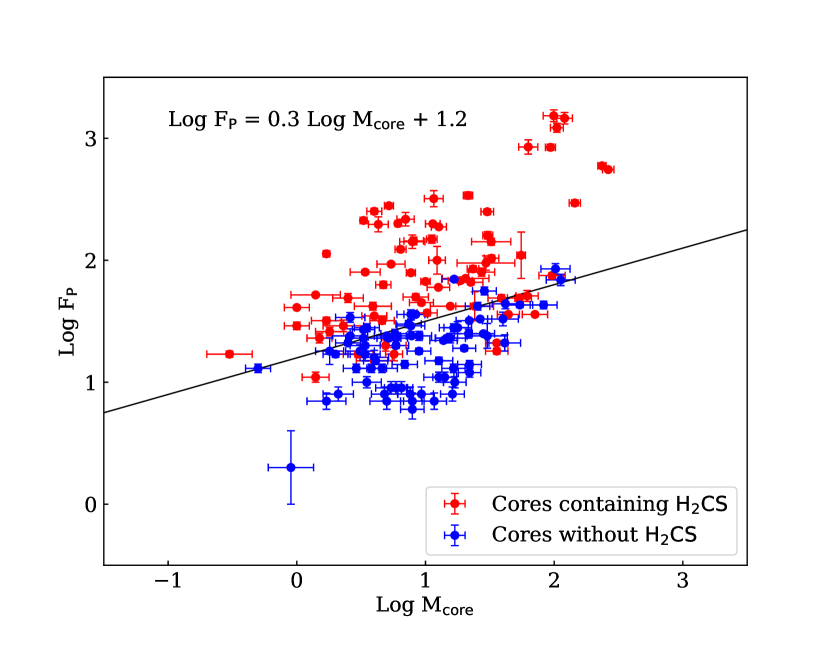
Here we define line-rich cores as those with abundant molecular spectral lines (at least 50 lines) and potential CH3OCHO detection (Kurtz et al., 2000; Ceccarelli, 2004; Jørgensen et al., 2020). Warm cores have H2CS detection but no CH3OCHO detection. Cold cores have only one or no H2CS line. Among the 145 cores, 28 cores are considered line-rich with at least 50 lines detected in SPWs 29 and 31 (Liu et al., 2023). Additionally, 25 less-line-rich cores (warm cores) and 92 cores with several molecular lines (cold cores) are also found. We used the XCLASS (Möller et al., 2017) software for H2CS line identification. Among the 145 cores, 72 have H2CS line emission. Multiple H2CS lines can be detected in all line-rich and warm cores, and 19 out of 92 cold cores only have single H2CS line transition. The reason whether a core has H2CS transition detected may be attributed to the relationship between the continuum peak flux (FP) and mass of the core (Mcore). Figure 2 illustrates 145 cores that the peak flux of 84.7% (61 out of 72) cores containing H2CS meets Log FP 0.3 Log Mcore + 1.2 and the peak flux of 84.9% (62 out of 73) cores without H2CS has Log FP 0.3 Log Mcore + 1.2.
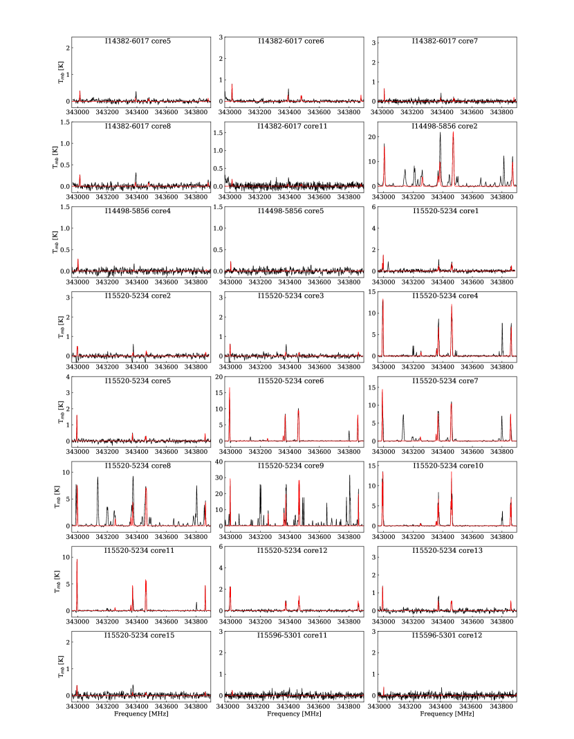
Figure 3 shows typical H2CS lines in I16076 for ”line-rich core”, ”warm core”, and ”cold core”. These three types of cores show different number and emission intensity of molecular lines. The fitting results of the other cores are shown in Figure A2.
| ID | IRAS | Core | FWHM | TypeaaColumn (9) presents the type of each core: G means neither H2CS nor CH3OCHO is detected; H means H2CS is detected but CH3OCHO is not detected; C means both H2CS and CH3OCHO are detected. | |||||||
|---|---|---|---|---|---|---|---|---|---|---|---|
| (″) | (K) | () | (km ) | (km ) | (K) | ( ) | |||||
| 1 | I14382-6017 | 5 | 1.13 | 47±14 | (6.8±3.5) | 2.0 | 59.8 | H | 0.1±0.0 | (6.2±3.2) | |
| 2 | I14382-6017 | 6 | 1.22 | 56±16 | (1.6±0.3) | 2.6 | 59.2 | H | 2.2±0.7 | (7.3±2.5) | |
| 3 | I14382-6017 | 7 | 1.34 | 50±17 | (7.1±0.2) | 1.4 | 59.2 | H | 1.2±0.4 | (6.1±2.1) | |
| 4 | I14382-6017 | 8 | 1.48 | 50±15 | (5.5±1.1) | 3.0 | 59.7 | H | 0.7±0.2 | (7.6±2.8) | |
| 5 | I14382-6017 | 11 | 1.37 | 51±5 | (4.1±2.6) | 3.0 | 59.2 | H | 1.8±0.2 | (2.3±1.5) | |
| 6 | I14498-5856 | 2 | 2.47 | 109±4 | (7.0±0.1) | 6.1 | 51.3 | C | 102±6 | 2.1±0.2 | (3.4±0.3) |
| 7 | I14498-5856 | 4 | 1.55 | 26±5 | (1.1±0.2) | 3.3 | 48.8 | G | 2.5±0.5 | (4.5±1.2) | |
| 8 | I14498-5856 | 5 | 1.63 | 26±5 | (6.0±1.5) | 2.0 | 47.5 | G | 1.9±0.4 | (3.2±1.0) | |
| 9 | I15520-5234 | 1 | 2.22 | 60±16 | (1.0±0.2) | 2.4 | 40.3 | H | 0.7±0.2 | (4.4±1.1) | |
| 55±11 | (2.1±0.2) | 2.5 | 44.7 | ||||||||
| 10 | I15520-5234 | 2 | 0.75 | 60±14 | (1.3±0.2) | 2.5 | 46.2 | H | 1.5±0.4 | (1.7±0.6) | |
| 43±13 | (1.2±0.4) | 2.3 | 43.1 | ||||||||
| 11 | I15520-5234 | 3 | 1.61 | 50±8 | (1.1±0.2) | 3.0 | 43.7 | H | 0.5±0.1 | (2.3±1.1) | |
| 12 | I15520-5234 | 4 | 3.04 | 78±7 | (2.7±0.1) | 3.5 | 43.5 | C | 77±11 | 2.7±0.3 | (1.5±0.1) |
| 64±8 | (1.3±0.1) | 3.2 | 39.7 | ||||||||
| 13 | I15520-5234 | 5 | 1.21 | 42±10 | (3.1±1.5) | 2.3 | 42.0 | H | 1.0±0.2 | (3.2±1.8) | |
| 14 | I15520-5234 | 6 | 2.41 | 70±3 | (3.6±0.1) | 3.4 | 40.5 | C | 80±10 | 1.6±0.1 | (2.3±0.2) |
| 15 | I15520-5234 | 7 | 1.45 | 79±3 | (4.1±0.1) | 3.8 | 39.6 | C | 78±10 | 2.8±0.4 | (1.5±0.2) |
| 16 | I15520-5234 | 8 | 1.39 | 100±4 | (2.2±0.3) | 3.8 | 44.2 | C | 104±6 | 1.9±0.3 | (1.2±0.3) |
| 17 | I15520-5234 | 9 | 1.67 | 107±4 | (5.6±0.1) | 1.8 | 44.3 | C | 102±4 | 1.8±0.1 | (3.1±0.2) |
| 18 | I15520-5234 | 10 | 1.63 | 74±18 | (1.9±0.1) | 2.6 | 39.1 | C | 70±36 | 1.1±0.2 | (3.5±0.4) |
| 63±11 | (1.8±0.2) | 1.6 | 42.8 | ||||||||
| 19 | I15520-5234 | 11 | 2.43 | 75±12 | (1.6±0.2) | 2.7 | 42.9 | C | 105±37 | 1.1±0.2 | (1.4±0.3) |
| 20 | I15520-5234 | 12 | 1.91 | 62±14 | (3.0±1.3) | 2.4 | 42.5 | H | 0.4±0.1 | (1.7±0.4) | |
| 46±13 | (3.8±1.0) | 2.7 | 46.1 | ||||||||
| 21 | I15520-5234 | 13 | 2.20 | 60±16 | (2.3±0.5) | 3.0 | 41.0 | H | 0.5±0.1 | (4.9±1.8) | |
| 22 | I15520-5234 | 15 | 1.04 | 50±9 | (8.2±4.0) | 2.7 | 42.7 | H | 0.8±0.2 | (1.1±0.6) | |
| 23 | I15596-5301 | 11 | 1.19 | 28±5 | (8.4±1.8) | 2.8 | 72.9 | G | 2.4±0.4 | (3.4±1.0) | |
| 24 | I15596-5301 | 12 | 1.09 | 28±5 | (5.6±1.2) | 0.7 | 72.5 | G | 2.5±0.5 | (2.2±0.6) | |
| 25 | I15596-5301 | 13 | 1.02 | 80±8 | (1.7±0.2) | 4.5 | 73.0 | C | 100±23 | 0.7±0.1 | (2.4±0.5) |
| 26 | I15596-5301 | 15 | 1.17 | 28±5 | (1.7±0.4) | 1.2 | 71.6 | G | 1.9±0.3 | (8.8±2.6) | |
| 27 | I15596-5301 | 16 | 1.50 | 28±5 | (9.5±2.1) | 2.3 | 71.2 | G | 0.9±0.2 | (1.0±0.3) | |
| 28 | I15596-5301 | 17 | 1.73 | 85±8 | (1.5±0.1) | 3.0 | 77.7 | H | 0.5±0.1 | (3.8±0.9) | |
| 66±13 | (3.2±0.2) | 2.4 | 73.0 | ||||||||
| 29 | I15596-5301 | 18 | 1.41 | 99±3 | (4.7±0.5) | 5.2 | 71.3 | C | 110±39 | 1.7±0.1 | (2.8±0.4) |
| 30 | I15596-5301 | 20 | 0.70 | 50±18 | (5.0±0.1) | 4.5 | 74.9 | H | 3.7±1.5 | (1.4±0.6) | |
| 31 | I15596-5301 | 21 | 1.66 | 28±5 | (1.9±0.4) | 2.8 | 74.9 | G | 0.8±0.1 | (2.5±0.7) | |
| 32 | I16060-5146 | 2 | 1.33 | 32±6 | (5.8±1.0) | 1.5 | 93.4 | G | 2.8±0.5 | (2.1±0.6) | |
| 33 | I16060-5146 | 4 | 1.33 | 110±13 | (4.7±0.1) | 4.7 | 96.5 | C | 136±4 | 12.1±2.1 | (3.9±0.7) |
| 34 | I16060-5146 | 5 | 1.62 | 110±6 | (5.6±0.1) | 3.0 | 84.8 | C | 112±7 | 7.6±0.7 | (7.3±0.6) |
| 35 | I16060-5146 | 7 | 1.44 | 121±4 | (1.2±0.3) | 6.4 | 95.8 | H | 12.5±1.6 | (9.6±2.7) | |
| 36 | I16060-5146 | 8 | 1.39 | 93±4 | (1.6±0.1) | 6.4 | 86.3 | C | 110±2 | 11.8±1.3 | (1.4±0.2) |
| 37 | I16060-5146 | 9 | 0.92 | 86±11 | (2.0±0.1) | 4.4 | 92.9 | H | 3.3±0.5 | (1.1±0.1) | |
| 81±9 | (1.7±0.1) | 5.2 | 86.9 | ||||||||
| 38 | I16060-5146 | 10 | 0.94 | 32±6 | (9.8±1.7) | 1.5 | 87.8 | G | 2.3±0.4 | (4.3±1.1) | |
| 39 | I16060-5146 | 11 | 1.43 | 40±3 | (1.3±0.1) | 2.7 | 97.4 | H | 2.5±0.2 | (5.3±0.7) | |
| 40 | I16060-5146 | 12 | 1.10 | 32±6 | (2.7±0.5) | 2.5 | 94.3 | G | 3.3±0.6 | (8.1±2.2) | |
| 41 | I16060-5146 | 13 | 1.55 | 46±7 | (2.7±1.0) | 2.2 | 92.4 | H | 0.9±0.2 | (2.9±1.2) | |
| 42 | I16071-5142 | 5 | 0.59 | 23±4 | (4.5±1.3) | 3.5 | 84.4 | G | 7.8±1.4 | (5.8±2.0) | |
| 43 | I16071-5142 | 6 | 1.34 | 95±4 | (2.6±0.1) | 8.7 | 87.2 | C | 127±10 | 7.5±1.2 | (3.5±0.6) |
| 44 | I16076-5134 | 8 | 1.98 | 30±6 | (1.2±0.3) | 2.4 | 86.1 | G | 2.1±0.5 | (5.6±1.8) | |
| 45 | I16076-5134 | 9 | 0.94 | 81±18 | (4.5±1.5) | 3.2 | 89.5 | C | 87±11 | 1.9±0.4 | (2.4±1.0) |
| 46 | I16076-5134 | 10 | 2.30 | 81±8 | (8.9±1.0) | 5.6 | 86.4 | H | 0.2±0.0 | (3.9±0.7) | |
| 47 | I16076-5134 | 11 | 1.86 | 98±3 | (7.1±0.1) | 8.5 | 87.2 | C | 98±10 | 1.9±0.2 | (3.7±0.3) |
| 48 | I16076-5134 | 12 | 1.20 | 42±12 | (1.4±0.6) | 1.3 | 89.9 | H | 0.7±0.2 | (1.9±1.0) | |
| 49 | I16076-5134 | 14 | 0.92 | 30±6 | (2.8±0.6) | 3.5 | 87.2 | G | 1.0±0.3 | (2.7±1.0) | |
| 50 | I16076-5134 | 15 | 1.28 | 68±5 | (8.4±1.2) | 3.0 | 87.4 | H | 1.3±0.1 | (6.4±1.1) | |
| 51 | I16272-4837 | 4 | 0.89 | 89±3 | (1.5±0.1) | 3.2 | 46.6 | C | 106±3 | 3.0±0.2 | (5.1±0.5) |
| 52 | I16272-4837 | 5 | 1.16 | 23±4 | (8.5±2.5) | 2.0 | 45.5 | G | 2.5±0.5 | (3.5±1.2) | |
| 53 | I16272-4837 | 6 | 0.85 | 90±9 | (6.8±0.2) | 8.0 | 48.4 | C | 102±17 | 4.0±0.5 | (1.7±0.2) |
| 54 | I16272-4837 | 7 | 0.81 | 71±5 | (1.4±0.1) | 2.4 | 46.4 | C | 82±27 | 5.7±0.4 | (2.5±0.3) |
| 55 | I16272-4837 | 8 | 0.80 | 112±6 | (3.6±0.1) | 3.1 | 46.4 | C | 115±4 | 15.7±1.3 | (2.3±0.2) |
| 56 | I16351-4722 | 4 | 0.69 | 70±5 | (8.4±0.3) | 1.8 | 42.0 | C | 90±9 | 2.4±0.2 | (3.5±0.3) |
| 57 | I16351-4722 | 5 | 1.25 | 30±6 | (9.8±2.0) | 1.5 | 42.4 | G | 1.8±0.4 | (5.5±1.6) | |
| 58 | I16351-4722 | 6 | 1.74 | 87±12 | (3.0±0.2) | 4.8 | 43.3 | C | 70±4 | 1.8±0.3 | (2.0±0.3) |
| 76±18 | (5.3±0.2) | 2.2 | 38.1 | ||||||||
| 59 | I16351-4722 | 7 | 2.04 | 101±1 | (3.0±0.1) | 5.5 | 39.6 | C | 170±10 | 1.9±0.3 | (1.6±0.3) |
| 60 | I16351-4722 | 8 | 1.83 | 81±10 | (5.6±0.3) | 4.8 | 39.0 | C | 91±4 | 2.3±0.3 | (2.5±0.3) |
| 61 | I16351-4722 | 9 | 1.76 | 56±4 | (4.8±0.2) | 1.0 | 37.7 | H | 1.6±0.1 | (3.0±0.3) | |
| 62 | I16351-4722 | 10 | 1.33 | 58±7 | (4.2±0.8) | 4.0 | 38.1 | H | 1.8±0.2 | (2.4±0.6) | |
| 63 | I16351-4722 | 11 | 0.70 | 78±5 | (4.7±0.1) | 3.0 | 37.6 | H | 0.4±0.0 | (1.1±0.1) | |
| 64 | I16351-4722 | 12 | 1.10 | 51±12 | (3.4±1.1) | 3.9 | 40.1 | H | 1.4±0.3 | (2.4±1.0) | |
| 65 | I17204-3636 | 4 | 0.98 | 25±5 | (1.8±0.5) | 3.0 | 16.9 | G | 0.8±0.2 | (2.2±0.8) | |
| 66 | I17204-3636 | 5 | 1.28 | 25±5 | (7.0±2.0) | 2.0 | 16.9 | G | 1.0±0.2 | (6.9±2.5) | |
| 67 | I17204-3636 | 9 | 1.55 | 88±7 | (3.0±0.2) | 3.0 | 17.5 | H | 1.5±0.1 | (2.0±0.2) | |
| 68 | I17220-3609 | 3 | 1.48 | 25±5 | (2.4±0.7) | 2.5 | 94.1 | G | 4.1±0.9 | (5.8±2.1) | |
| 69 | I17220-3609 | 7 | 1.70 | 68±5 | (3.8±0.6) | 5.0 | 94.6 | H | 4.8±0.5 | (8.0±1.5) | |
| 70 | I17220-3609 | 9 | 2.24 | 100±9 | (2.5±0.1) | 7.2 | 96.1 | C | 107±13 | 4.9±0.5 | (5.1±0.5) |
| 71 | I17220-3609 | 10 | 1.84 | 117±6 | (2.4±1.2) | 7.4 | 96.7 | C | 94±3 | 6.6±0.5 | (3.7±1.8) |
| 72 | I17220-3609 | 14 | 1.91 | 25±5 | (1.5±0.4) | 3.0 | 95.1 | G | 1.8±0.4 | (8.2±2.7) |
Note. — IRAS sources and extracted cores ID are listed in column (2) and (3). The calculated deconvolved source sizes are listed in column (4). The fitted rotational temperatures, column densities, FWHM, and velocity offset () of H2CS are listed in column (5)–(8), for 8 cores with two velocity components, the parameters are listed simultaneously. The fitted rotational temperatures of CH3OCHO are list in column (10) (C. Li et al. 2023, submitted to ApJ). The peak column densities of H2 are shown in column (11) and the abundances of H2CS relative to H2 are shown in column (12).

3.3 H2CS Spatial Distribution
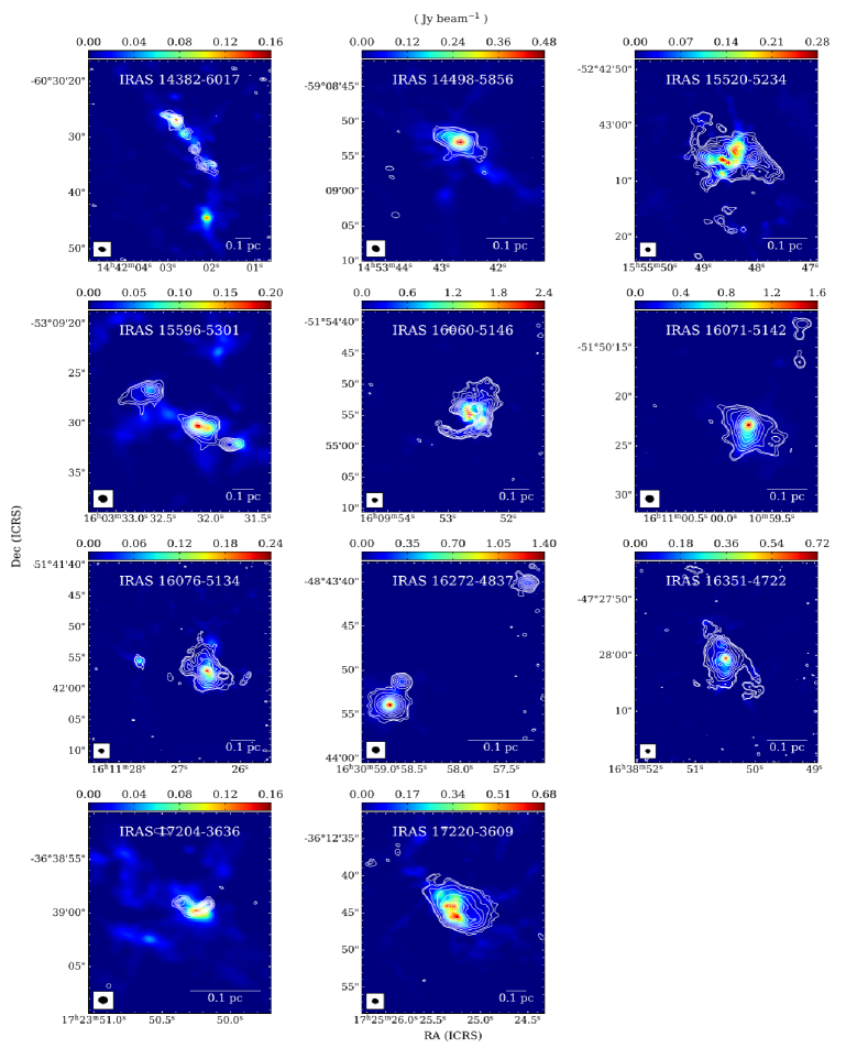
Figure 4 shows the 870 m continuum maps of the 11 protocluster clumps, overlaid with contours of the H2CS Moment 0 (integrated intensity) maps. For the continuum maps, we zoom in on the central regions of the protoclusters to see the intensities of H2CS emissions in detail. The moment 0 maps demonstrate that H2CS is widely distributed throughout the clumps.
Among our targeted 11 sources, I14382 and I17204 are 2 sources with a few molecular emission lines and only contain warm cores and cold cores, and H2CS is distributed within very small areas around warm cores. For the two sources I14498 and I15596, the emissions of H2CS molecule are mainly around the compact regions of the line-rich cores. And for the remaining 7 sources, the spatial distribution of H2CS emission is similar with the dust emission. The observations revealed that the emission of H2CS is originated from extended regions surrounding both compact line-rich cores and warm cores and also can cover plenty of regions of the cold cores.
3.4 Temperature Structure
Temperature is an indicator of the interstellar chemical complexity and star formation process (Sánchez-Monge et al., 2017; Gorai et al., 2020; Liu et al., 2020a; Peng et al., 2022). It affects the mass estimation of dense gas. It also provides the main thermal pressure source within molecular gas (Rosen et al., 2020; Rosen, 2022), which counteracts gravity in the early stages of star formation. Thus, accurate temperature measurements enable an appropriate understanding of star formation mechanism. H2CS can provide such an useful tracer of gas temperature.
Table 3 lists the number of these three-type cores. The H2CS temperature ranges from 23 to 121 K for all cores. The range is 68 to 121 K for line-rich cores and 40 to 88 K for warm cores. The temperatures for cold cores range from 23 to 32 K, which are equal to the clump temperatures. Compared to the temperatures of CH3OCHO of line-rich cores, H2CS shows no significant temperature differences within uncertainties, because the molecule is thermalized in line-rich core regions. Therefore, we choose the higher gas temperature of H2CS and CH3OCHO as . In addition, H2CS is more widely distributed than CH3OCHO in protoclusters and can applicably determine the temperature of cold cores, warm cores and line-rich cores, indicating that H2CS is a more efficient temperature tracer as it can trace more extended regions than CH3OCHO.
| Sources | Cores | Total | ||
|---|---|---|---|---|
| Line-rich | Warm | Cold | ||
| IRAS 14382-6017 | 0 | 5 | 6 | 11 |
| IRAS 14498-5856 | 1 | 0 | 6 | 7 |
| IRAS 15520-5234 | 7 | 7 | 1 | 15 |
| IRAS 15596-5301 | 2 | 2 | 23 | 27 |
| IRAS 16060-5146 | 4 | 3 | 6 | 13 |
| IRAS 16071-5142 | 1 | 0 | 6 | 7 |
| IRAS 16076-5134 | 2 | 3 | 10 | 15 |
| IRAS 16272-4837 | 4 | 0 | 5 | 9 |
| IRAS 16351-4722 | 4 | 4 | 4 | 12 |
| IRAS 17204-3636 | 0 | 1 | 11 | 12 |
| IRAS 17220-3609 | 3 | 0 | 14 | 17 |
| Total | 28 | 25 | 92 | 145 |
4 Discussion
4.1 H2CS Column Densities and Abundances
Based on Table 2 and Figure 5, several significant characteristics can be found among line-rich, warm, and cold cores by comparing and parameters. For line-rich cores, ranges from to , with a mean of . For warm and cold cores, ranges from to and to , with means of and , respectively. The line-rich cores have higher values than the other two types of cores. The warm cores have a wider range of than the cold ones, but the values overlap, despite the mean of warm cores being much higher (about twice) than that of cold cores.
The abundance of H2CS versus H2 () is calculated via /. Apparently, varies similarly to . Numerous studies have analyzed and in diverse massive star formation regions. Table A3 lists the results of previous studies on H2CS in line-rich cores of massive star formation regions. We combine these 7 line-rich cores with our 28 line-rich core samples, resulting in 35 line-rich core samples. Among the line-rich cores, Mon R 2 IRS 3 A (Fuente et al., 2021) and Sgr B2 (Möller et al., 2021) have lower than the line-rich cores studied here. Except for these 2 line-rich cores, the other 33 have similar ranges from to . These results indicate that varies greatly among different line-rich cores within and outside the Galaxy.
Similarly, due to physical differences, can vary greatly among different interstellar environments, leading to variation in . It is worth noting that I16351 core7 has a very high of . The reason for this large value is its high and low . Except for this line-rich core, the abundance values of the other 34 are within the same range, from to .
4.2 Temperature-Abundance Relation
Through the results collated in Table 2, we can clearly find that temperature has a significant effect on the value of H2CS abundance. Considering two variables X and Y, the formula for Pearson’s correlation coefficient r can be expressed as:
| (4) |
where and are the mean values of X and Y. The value of Pearson’s correlation coefficient for temperature and is 0.71. The value of relies on temperature, and the corresponding trend line shown in left panel of Figure 5 is fitted as,
| (5) |
with uncertainties of 9.4% and 1.3% for slope and intercept. We find the abundance tends to increase with increasing temperature. H2CS molecule is thought to be trapped on icy dust grains and principally form on dust grain surface at low temperatures (Jørgensen et al., 2020), and is generally desorbed from the grain surface into gas-phase as the temperature increases (Vidal & Wakelam, 2018; Vidal et al., 2019). The chemical property of H2CS in the hot regions is to a high degree inherited from the surrounding cold dust regions (el Akel et al., 2022). Therefore would be a good tracer of gas temperature.
4.3 Column Density-Abundance Relation


Since and show the same trend in all types of cores, it would be pertinent to discuss the relationship of and . The value of Pearson’s correlation coefficient for and is 0.88, indicating a high correlation between H2CS and H2.
The correlation between and is shown in right panel of Figure 5. We can see that is sensitive to changes in . Thus, the trend line of and can be expressed using the following equation,
| (6) |
with uncertainties of 5.3% and 3.1% for slope and intercepts. The red dots represent line-rich cores that have abundant organic molecules and high temperatures, column densities, and abundances of H2CS. The line-rich cores have higher and than warm cores and cold cores. Additionally, warm cores are largely scattered above the line, while cold cores are below the line. This indicates that warm cores have higher than cold cores at same .
This trend suggests that different regions have varying chemical characteristics and that the H2CS abundances are enhanced from cold cores, warm cores to line-rich cores. Additionally, this proportional relationship can provide insights into the distribution and formation of H2CS in interstellar space. Further observations and studies are still needed to better understand the physical and chemical properties of H2CS in space.
5 Conclusions
We have presented the continuum and H2CS line observations using the ALMA Band-7 survey toward 11 massive protocluster sources. The observations have detected a total of 145 continuum dense cores. Of these, 72 have H2CS emission, including 28 line-rich cores, 25 warm cores, and 19 cold cores. The major results are summarized as follows:
(1) 72 cores with H2CS in our sample have column densities exceed a threshold value for star formation, stating that H2CS can be widely distributed in star-forming regions with different physical environments.
(2) Spatial distribution of H2CS are revealed among the 11 sources. H2CS emissions come from extended areas around dense rich-line cores and warm cores, and can also cover large areas of cold cores.
(3) H2CS is found extensively distributed in protoclusters and increases with temperature from cold cores, warm cores to line-rich cores, indicating that H2CS is a good tracer for temperature in a variety of complex physical environments.
(4) and are found tightly correlated among different types of cores, showing that the H2CS abundances are enhanced from cold cores, warm cores to line-rich cores in star forming regions.
Our ALMA observations of the H2CS line provide a substantial dataset of massive protoclusters with high angular resolution, which plays a crucial role in studying the formation mechanism and spatial distribution of H2CS in interstellar space. Further observations and studies will definitely enhance our understanding of the H2CS formation network and contribute to advancements in astrochemistry.
Appendix A Cores identification and 2D Gaussian fitting
The complete results of cores identification of the 11 IRAS sources are shown in Figure 1 and Figure A1. The background color maps show the ALMA 345 GHz continuum flux in J2000.0 coordinates. The overlaid black contours of flux start from 8 rms and increase with power-law function. Each central location of identified cloud core is marked with yellow cross and the corresponding ID number is labeled beside the cross. The deconvolved parameters of each core was obtained from 2D Gaussian fitting tool in CASA and the whole parameters of the 145 cores are list in Table A2.
Appendix B The fitted H2CS spectral lines
Figure A2 illustrates the 72 observed molecular lines and the synthetic spectra of the best fitting parameters for H2CS lines. All the nine transitions of H2CS surveyed in ALMA Band-7, which are summarized in Table A2, are only tuned in SPW 31 and so here we present frequency range from roughly 342.95 GHz to 344.00 GHz.


| ID | IRAS | Core | RA | DEC | Source size | PA | Mass | Integrated flux | Peak intensity | Note |
|---|---|---|---|---|---|---|---|---|---|---|
| () | (∘) | () | (mJy) | (mJy beam-1) | ||||||
| 1 | I14382-6017 | 1 | 14:42:03.6 | 60:30:10.4 | 1.51.3 | 51 | 25.4±5.0 | 127±11 | 42±3 | |
| 2 | I14382-6017 | 2 | 14:42:02.5 | 60:30:10.2 | 2.41.1 | 100 | 26.6±5.0 | 133±7 | 33±1 | |
| 3 | I14382-6017 | 3 | 14:42:01.9 | 60:30:09.6 | 1.20.6 | 68 | 4.6±1.1 | 23±4 | 13±1 | |
| 4 | I14382-6017 | 4 | 14:42:02.9 | 60:30:22.8 | 1.00.6 | 90 | 7.8±1.4 | 39±2 | 24±1 | |
| 5 | I14382-6017 | 5 | 14:42:03.1 | 60:30:26.1 | 1.60.8 | 69 | 1.4±0.5 | 13±3 | 52±1 | |
| 6 | I14382-6017 | 6 | 14:42:02.8 | 60:30:27.3 | 1.51.0 | 33 | 32.4±9.6 | 380±30 | 142±9 | |
| 7 | I14382-6017 | 7 | 14:42:02.6 | 60:30:29.5 | 1.51.2 | 43 | 20.5±7.0 | 210±8 | 71±2 | |
| 8 | I14382-6017 | 8 | 14:42:02.4 | 60:30:31.3 | 2.21.0 | 10 | 15.6±4.7 | 160±6 | 42±1 | |
| 9 | I14382-6017 | 9 | 14:42:02.1 | 60:30:34.8 | 2.81.3 | 65 | 41.8±8.8 | 209±23 | 44±4 | |
| 10 | I14382-6017 | 10 | 14:42:02.0 | 60:30:36.8 | 1.90.9 | 18 | 14.6±2.6 | 73±2 | 23±1 | |
| 11 | I14382-6017 | 11 | 14:42:02.1 | 60:30:44.5 | 1.71.1 | 174 | 32.6±4.0 | 343±26 | 104±6 | |
| 12 | I14498-5859 | 1 | 14:53:42:4 | 59:08:46.1 | 3.61.3 | 144 | 4.1±0.8 | 108±8 | 15±1 | |
| 13 | I14498-5859 | 2 | 14:53:42.7 | 59:08:52:8 | 3.21.9 | 65 | 21.4±1.7 | 2830±200 | 340±22 | * |
| 14 | I14498-5859 | 3 | 14:53:42.8 | 59:08:57.7 | 1.61.5 | 40 | 3.3±0.9 | 87±17 | 23±4 | |
| 15 | I14498-5859 | 4 | 14:53:42.2 | 59:08:57.2 | 4.11.6 | 57 | 27.3±5.7 | 716±60 | 80±6 | |
| 16 | I14498-5859 | 5 | 14:53:42.9 | 59:09:00.6 | 1.91.4 | 148 | 8.4±1.7 | 219±15 | 50±3 | |
| 17 | I14498-5859 | 6 | 14:53:41.6 | 59:09:00.2 | 3.01.5 | 50 | 7.4±1.5 | 193±14 | 30±2 | |
| 18 | I14498-5859 | 7 | 14:53:40.3 | 59:09:06.0 | 2.81.6 | 121 | 4.0±0.9 | 104±11 | 16±2 | |
| 19 | I15520-5234 | 1 | 15:55:49.1 | 52:42:59.2 | 2.91.7 | 40 | 3.9±1.1 | 399±31 | 42±3 | |
| 20 | I15520-5234 | 2 | 15:55:48.8 | 52:43:01.7 | 1.40.4 | 16 | 1.0±0.2 | 99±4 | 41±1 | |
| 21 | I15520-5234 | 3 | 15:55:49.3 | 52:43:02.9 | 2.01.3 | 115 | 1.5±0.3 | 128±13 | 23±2 | |
| 22 | I15520-5234 | 4 | 15:55:48.4 | 52:43:04.2 | 3.72.5 | 19 | 30.2±3.2 | 4130±230 | 250±13 | * |
| 23 | I15520-5234 | 5 | 15:55:49.3 | 52:43:05.7 | 2.10.7 | 87 | 1.7±0.4 | 115±7 | 32±2 | |
| 24 | I15520-5234 | 6 | 15:55:48.9 | 52:43:06.1 | 2.92.0 | 158 | 11.2±1.0 | 1600±120 | 149±11 | * |
| 25 | I15520-5234 | 7 | 15:55:48.7 | 52:43:06.1 | 1.91.1 | 76 | 7.0±1.0 | 968±137 | 217±26 | * |
| 26 | I15520-5234 | 8 | 15:55:48.5 | 52:43:06.8 | 1.61.2 | 60 | 4.3±0.7 | 819±133 | 197±26 | * |
| 27 | I15520-5234 | 9 | 15:55:48.4 | 52:43:06.5 | 2.01.4 | 119 | 6.1±0.3 | 1128±35 | 200±5 | * |
| 28 | I15520-5234 | 10 | 15:55:48.1 | 52:43:06.5 | 1.91.4 | 85 | 3.4±0.8 | 440±18 | 80±3 | * |
| 29 | I15520-5234 | 11 | 15:55:48.6 | 52:43:08.5 | 3.11.9 | 63 | 7.9±1.6 | 1510±190 | 142±17 | * |
| 30 | I15520-5234 | 12 | 15:55:47.8 | 52:43:09.7 | 2.81.3 | 23 | 1.8±0.4 | 190±19 | 26±2 | |
| 31 | I15520-5234 | 13 | 15:55:48.3 | 52:43:18.6 | 3.41.2 | 80 | 2.3±0.7 | 234±27 | 29±3 | |
| 32 | I15520-5234 | 14 | 15:55:47.8 | 52:43:18.3 | 2.60.8 | 0 | 2.6±0.7 | 125±21 | 24±3 | |
| 33 | I15520-5234 | 15 | 15:55:47.5 | 52:43:17.1 | 1.20.9 | 88 | 1.0±0.2 | 81±8 | 29±2 | |
| 34 | I15596-5301 | 1 | 16:03:32.7 | 53:09:08.2 | 2.01.1 | 117 | 11.7±2.3 | 34±3 | 7±1 | |
| 35 | I15596-5301 | 2 | 16:03:33.3 | 53:09:10.2 | 1.20.9 | 167 | 7.6±1.5 | 22±2 | 8±1 | |
| 36 | I15596-5301 | 3 | 16:03:33.1 | 53:09:12.6 | 1.90.7 | 62 | 14.1±2.7 | 41±3 | 11±1 | |
| 37 | I15596-5301 | 4 | 16:03:32.4 | 53:09:13.0 | 1.70.8 | 145 | 7.9±1.5 | 23±1 | 6±1 | |
| 38 | I15596-5301 | 5 | 16:03:32.4 | 53:09:14.1 | 1.60.8 | 55 | 9.3±1.8 | 27±2 | 8±1 | |
| 39 | I15596-5301 | 6 | 16:03:29.9 | 53:09:15.2 | 0.70.3 | 116 | 8.9±1.7 | 26±2 | 18±1 | |
| 40 | I15596-5301 | 7 | 16:03:32.9 | 53:09:19.5 | 1.60.7 | 111 | 28.2±5.1 | 82±2 | 25±1 | |
| 41 | I15596-5301 | 8 | 16:03:33.2 | 53:09:21.1 | 1.91.0 | 12 | 22.0±4.2 | 64±4 | 14±1 | |
| 42 | I15596-5301 | 9 | 16:03:33.2 | 53:09:22.2 | 2.01.0 | 115 | 16.9±3.1 | 49±2 | 10±1 | |
| 43 | I15596-5301 | 10 | 16:03:31.8 | 53:09:18.8 | 1.00.7 | 24 | 6.5±1.2 | 19±1 | 9±1 | |
| 44 | I15596-5301 | 11 | 16:03:32.6 | 53:09:26.7 | 1.51.0 | 76 | 61.6±11.1 | 179±4 | 51±5 | |
| 45 | I15596-5301 | 12 | 16:03:31.9 | 53:09:22.8 | 1.40.9 | 139 | 53.7±10.4 | 156±12 | 49±3 | |
| 46 | I15596-5301 | 13 | 16:03:32.6 | 53:09:26.6 | 1.30.8 | 67 | 12.3±1.7 | 160±16 | 100±23 | * |
| 47 | I15596-5301 | 14 | 16:03:32.8 | 53:09:27.5 | 1.60.6 | 16 | 20.0±3.7 | 58±3 | 19±1 | |
| 48 | I15596-5301 | 15 | 16:03:32.7 | 53:09:29.3 | 1.50.9 | 177 | 44.1±7.9 | 128±3 | 36±1 | |
| 49 | I15596-5301 | 16 | 16:03:32.9 | 53:09:31.1 | 1.81.3 | 101 | 35.8±6.5 | 104±4 | 21±1 | |
| 50 | I15596-5301 | 17 | 16:03:32.4 | 53:09:29.1 | 2.31.3 | 60 | 24.1±6.9 | 263±71 | 42±10 | |
| 51 | I15596-5301 | 18 | 16:03:32.1 | 53:09:30.3 | 2.20.9 | 66 | 55.4±4.1 | 799±54 | 110±39 | * |
| 52 | I15596-5301 | 19 | 16:03:31.7 | 53:09:28.3 | 0.70.3 | 24 | 6.9±1.4 | 20±2 | 14±1 | |
| 53 | I15596-5301 | 20 | 16:03:31.7 | 53:09:32.1 | 0.80.6 | 63 | 29.5±11.9 | 176±32 | 95±12 | |
| 54 | I15596-5301 | 21 | 16:03:32.1 | 53:09:33.7 | 2.01.4 | 12 | 35.8±6.5 | 104±4 | 18±1 | |
| 55 | I15596-5301 | 22 | 16:03:31.4 | 53:09:33.1 | 1.41.1 | 91 | 16.5±3.1 | 48±3 | 13±1 | |
| 56 | I15596-5301 | 23 | 16:03:31.3 | 53:09:32.9 | 1.91.3 | 65 | 22.0±4.0 | 64±2 | 12±1 | |
| 57 | I15596-5301 | 24 | 16:03:30.7 | 53:09:33.8 | 1.20.7 | 70 | 12.7±2.8 | 37±5 | 15±1 | |
| 58 | I15596-5301 | 25 | 16:03:30.5 | 53:09:35.6 | 1.00.5 | 75 | 5.9±1.1 | 17±1 | 9±1 | |
| 59 | I15596-5301 | 26 | 16:03:30.2 | 53:09:34.3 | 2.10.4 | 79 | 7.9±1.5 | 23±1 | 7±1 | |
| 60 | I15596-5301 | 27 | 16:03:32.4 | 53:09:41.9 | 2.31.0 | 7 | 16.2±3.1 | 47±3 | 8±1 | |
| 61 | I16060-5146 | 1 | 16:09:53.1 | 51:54:43.7 | 2.31.7 | 114 | 17.8±3.9 | 223±26 | 28±3 | |
| 62 | I16060-5146 | 2 | 16:09:53.1 | 51:54:53.2 | 1.61.1 | 119 | 22.5±4.4 | 282±16 | 66±3 | |
| 63 | I16060-5146 | 3 | 16:09:53.2 | 51:54:55.0 | 1.50.7 | 72 | 8.4±1.6 | 105±5 | 36±1 | |
| 64 | I16060-5146 | 4 | 16:09:52.7 | 51:54:53.9 | 1.61.1 | 11 | 99.2±17.0 | 6520±810 | 1530±160 | * |
| 65 | I16060-5146 | 5 | 16:09:52.4 | 51:54:53.8 | 2.21.2 | 34 | 93.6±8.0 | 5000±330 | 843±48 | * |
| 66 | I16060-5146 | 6 | 16:09:51.9 | 51:54:53.7 | 1.50.7 | 58 | 16.7±3.3 | 210±11 | 70±3 | |
| 67 | I16060-5146 | 7 | 16:09:52.6 | 51:54:55.2 | 1.61.3 | 177 | 120.5±15.7 | 6990±880 | 1460±150 | * |
| 68 | I16060-5146 | 8 | 16:09:52.4 | 51:54:55.6 | 1.61.2 | 142 | 105.0±11.4 | 5500±550 | 1220±100 | * |
| 69 | I16060-5146 | 9 | 16:09:53.0 | 51:54:57.4 | 1.40.6 | 83 | 12.7±1.6 | 507±8 | 188±2 | |
| 70 | I16060-5146 | 10 | 16:09:53.7 | 51:55:00.7 | 1.10.8 | 13 | 9.3±1.8 | 117±6 | 45±2 | |
| 71 | I16060-5146 | 11 | 16:09:53.5 | 51:54:59.0 | 1.71.2 | 80 | 23.4±2.3 | 389±25 | 85±5 | |
| 72 | I16060-5146 | 12 | 16:09:53.2 | 51:54:59.6 | 1.50.8 | 58 | 18.6±3.6 | 234±11 | 68±3 | |
| 73 | I16060-5146 | 13 | 16:09:52.6 | 51:55:02.4 | 2.01.2 | 137 | 10.3±1.7 | 203±12 | 37±2 | |
| 74 | I16071-5142 | 1 | 16:10:59.0 | 51:50:03.2 | 0.90.7 | 45 | 7.7±1.7 | 62±8 | 29±3 | |
| 75 | I16071-5142 | 2 | 16:10:59.4 | 51:50:06.9 | 1.50.4 | 50 | 5.9±1.2 | 48±5 | 20±1 | |
| 76 | I16071-5142 | 3 | 16:10:59.2 | 51:50:07.7 | 0.90.7 | 54 | 5.9±1.1 | 48±2 | 23±1 | |
| 77 | I16071-5142 | 4 | 16:10:59.3 | 51:50:10.5 | 2.10.6 | 180 | 28.7±5.5 | 232±18 | 56±4 | |
| 78 | I16071-5142 | 5 | 16:10:59.4 | 51:50:16.6 | 0.70.5 | 0 | 12.6±2.3 | 102±6 | 60±2 | |
| 79 | I16071-5142 | 6 | 16:10:59.8 | 51:50:23.1 | 1.81.0 | 164 | 62.9±9.9 | 3840±580 | 849±107 | * |
| 80 | I16071-5142 | 7 | 16:10:59.4 | 51:50:34.5 | 1.50.6 | 139 | 8.9±1.8 | 72±7 | 24±2 | |
| 81 | I16076-5134 | 1 | 16:11:28.6 | 51:41:44.9 | 2.01.4 | 57 | 5.4±1.3 | 62±9 | 9±1 | |
| 82 | I16076-5134 | 2 | 16:11:26.7 | 51:41:44.6 | 3.21.0 | 33 | 5.0±1.3 | 58±9 | 7±1 | |
| 83 | I16076-5134 | 3 | 16:11:25.8 | 51:41:44.9 | 1.20.6 | 149 | 2.1±0.5 | 24±4 | 8±1 | |
| 84 | I16076-5134 | 4 | 16:11:29.1 | 51:41:50.0 | 1.50.9 | 86 | 3.5±0.8 | 40±5 | 10±1 | |
| 85 | I16076-5134 | 5 | 16:11:26.8 | 51:41:50.7 | 2.00.8 | 69 | 0.9±0.3 | 10±2 | 2±1 | |
| 86 | I16076-5134 | 6 | 16:11:26.6 | 51:41:50.2 | 2.91.9 | 39 | 12.7±3.0 | 147±19 | 11±1 | |
| 87 | I16076-5134 | 7 | 16:11:26.4 | 51:41:50.2 | 2.21.2 | 161 | 4.8±1.0 | 55±1 | 8±1 | |
| 88 | I16076-5134 | 8 | 16:11:26.5 | 51:41:52.7 | 2.31.7 | 71 | 38.9±8.3 | 449±32 | 49±3 | |
| 89 | I16076-5134 | 9 | 16:11:27.7 | 51:41:55.6 | 0.90.7 | 69 | 5.4±1.2 | 218±5 | 93±1 | * |
| 90 | I16076-5134 | 10 | 16:11:26.9 | 51:41:56.7 | 3.11.7 | 18 | 5.7±0.8 | 214±21 | 17±2 | |
| 91 | I16076-5134 | 11 | 16:11:26.5 | 51:41:57.4 | 2.31.5 | 16 | 30.5±2.6 | 1410±110 | 160±11 | * |
| 92 | I16076-5134 | 12 | 16:11:26.2 | 51:41:57.3 | 1.80.8 | 70 | 4.9±1.5 | 86±10 | 20±2 | |
| 93 | I16076-5134 | 13 | 16:11:25.9 | 51:41:57.1 | 1.60.6 | 55 | 3.8±0.9 | 44±6 | 13±1 | |
| 94 | I16076-5134 | 14 | 16:11:25.9 | 51:41:58.3 | 1.40.6 | 151 | 4.0±1.1 | 46±9 | 15±1 | |
| 95 | I16076-5134 | 15 | 16:11:26.6 | 51:41:59.5 | 1.51.1 | 113 | 10.0±0.8 | 310±11 | 67±2 | |
| 96 | I16272-4837 | 1 | 16:30:57.9 | 48:43:40.4 | 2.60.9 | 125 | 5.2±1.0 | 139±8 | 23±1 | |
| 97 | I16272-4837 | 2 | 16:30:57.7 | 48:43:37.5 | 1.80.6 | 51 | 3.5±0.7 | 95±7 | 28±2 | |
| 98 | I16272-4837 | 3 | 16:30:57.6 | 48:43:38.3 | 1.40.8 | 110 | 2.5±0.5 | 67±4 | 21±1 | |
| 99 | I16272-4837 | 4 | 16:30:57.3 | 48:43:40.1 | 1.00.8 | 77 | 3.3±0.2 | 549±27 | 212±8 | * |
| 100 | I16272-4837 | 5 | 16:30:58.4 | 48:43:50.9 | 1.50.9 | 173 | 4.6±0.9 | 123±10 | 32±2 | |
| 101 | I16272-4837 | 6 | 16:30:58.6 | 48:43:51.4 | 1.20.6 | 146 | 4.0±0.5 | 638±49 | 252±14 | * |
| 102 | I16272-4837 | 7 | 16:30:58.7 | 48:43:52.6 | 1.10.6 | 128 | 5.2±0.4 | 658±19 | 280±6 | * |
| 103 | I16272-4837 | 8 | 16:30:58.8 | 48:43:54.0 | 0.80.8 | 161 | 14.0±1.2 | 2560±160 | 1144±51 | * |
| 104 | I16272-4837 | 9 | 16:30:58.4 | 48:43:56.7 | 1.80.5 | 35 | 3.3±0.6 | 88±4 | 27±1 | |
| 105 | I16351-4722 | 1 | 16:38:51.2 | 47:27:46.2 | 2.41.1 | 112 | 3.1±0.7 | 111±12 | 18±2 | |
| 106 | I16351-4722 | 2 | 16:38:50.3 | 47:27:47.1 | 1.10.8 | 167 | 2.6±0.6 | 95±10 | 34±3 | |
| 107 | I16351-4722 | 3 | 16:38:51.5 | 47:27:55.2 | 1.40.9 | 62 | 1.8±0.4 | 65±4 | 18±4 | |
| 108 | I16351-4722 | 4 | 16:38:50.8 | 47:27:54.1 | 0.80.6 | 52 | 1.7±0.1 | 220±9 | 113±3 | * |
| 109 | I16351-4722 | 5 | 16:38:50.4 | 47:27:54.7 | 1.51.0 | 118 | 4.0±0.8 | 146±4 | 35±1 | |
| 110 | I16351-4722 | 6 | 16:38:50.6 | 47:27:58.1 | 1.91.6 | 8 | 8.1±1.3 | 1024±79 | 144±10 | * |
| 111 | I16351-4722 | 7 | 16:38:50.5 | 47:28:00.8 | 2.21.9 | 180 | 11.6±1.8 | 3010±470 | 320±45 | * |
| 112 | I16351-4722 | 8 | 16:38:50.5 | 47:28:02.8 | 2.11.6 | 159 | 11.4±1.4 | 1511±36 | 199±4 | * |
| 113 | I16351-4722 | 9 | 16:38:50.6 | 47:28:05.3 | 2.71.2 | 119 | 7.7±0.6 | 597±10 | 79±1 | |
| 114 | I16351-4722 | 10 | 16:38:50.0 | 47:28:02.8 | 2.00.9 | 21 | 4.7±0.6 | 378±23 | 63±4 | |
| 115 | I16351-4722 | 11 | 16:38:49.9 | 47:28:06.2 | 0.80.6 | 22 | 0.3±0.1 | 33±1 | 17±1 | |
| 116 | I16351-4722 | 12 | 16:38:50.1 | 47:28:07.7 | 1.30.9 | 174 | 2.5±0.6 | 170±9 | 49±4 | |
| 117 | I17204-3636 | 1 | 17:23:51.0 | 36:38:55.0 | 1.70.9 | 71 | 3.4±0.8 | 80±8 | 20±2 | |
| 118 | I17204-3636 | 2 | 17:23:50.8 | 36:38:54.6 | 2.11.0 | 45 | 5.8±1.3 | 136±12 | 25±2 | |
| 119 | I17204-3636 | 3 | 17:23:50.3 | 36:38:54.1 | 0.80.7 | 88 | 0.5±0.1 | 11±2 | 13±1 | |
| 120 | I17204-3636 | 4 | 17:23:50.2 | 36:38:55.1 | 1.20.8 | 6 | 1.4±0.3 | 32±4 | 11±1 | |
| 121 | I17204-3636 | 5 | 17:23:50.1 | 36:38:56.0 | 1.51.1 | 8 | 3.0±0.7 | 70±6 | 17±1 | |
| 122 | I17204-3636 | 6 | 17:23:50.8 | 36:38:56.6 | 1.30.6 | 6 | 2.0±0.4 | 46±2 | 17±1 | |
| 123 | I17204-3636 | 7 | 17:23:50.7 | 36:38:58.4 | 1.71.1 | 20 | 3.4±0.8 | 79±10 | 17±2 | |
| 124 | I17204-3636 | 8 | 17:23:50.6 | 36:38:58.0 | 2.20.9 | 164 | 2.9±0.6 | 67±4 | 13±1 | |
| 125 | I17204-3636 | 9 | 17:23:50.2 | 36:38:59.9 | 2.01.2 | 74 | 6.4±0.6 | 680±38 | 123±6 | |
| 126 | I17204-3636 | 10 | 17:23:50.0 | 36:39:01.9 | 2.40.9 | 43 | 1.7±0.5 | 39±7 | 7±1 | |
| 127 | I17204-3636 | 11 | 17:23:50.8 | 36:39:01.9 | 2.01.0 | 73 | 5.0±1.0 | 117±4 | 24±1 | |
| 128 | I17204-3636 | 12 | 17:23:50.6 | 36:39:02.5 | 2.30.9 | 75 | 7.7±1.7 | 181±16 | 36±3 | |
| 129 | I17220-3609 | 1 | 17:25:23.9 | 36:12:30.4 | 2.00.9 | 176 | 102.4±23.5 | 407±46 | 85±8 | |
| 130 | I17220-3609 | 2 | 17:25:24.1 | 36:12:31.2 | 1.91.0 | 165 | 40.0±9.6 | 159±21 | 33±4 | |
| 131 | I17220-3609 | 3 | 17:25:25.6 | 36:12:35.0 | 2.01.1 | 134 | 96.3±20.2 | 383±24 | 75±4 | |
| 132 | I17220-3609 | 4 | 17:25:24.8 | 36:12:35.6 | 3.70.8 | 158 | 41.3±10.2 | 164±24 | 21±3 | |
| 133 | I17220-3609 | 5 | 17:25:24.5 | 36:12:39.3 | 1.60.4 | 158 | 21.9±4.6 | 87±5 | 32±1 | |
| 134 | I17220-3609 | 6 | 17:25:25.7 | 36:12:39.5 | 2.71.0 | 85 | 112.4±25.6 | 447±49 | 69±7 | |
| 135 | I17220-3609 | 7 | 17:25:25.4 | 36:12:42.6 | 1.81.6 | 105 | 144.7±13.8 | 1960±120 | 295±16 | * |
| 136 | I17220-3609 | 8 | 17:25:25.8 | 36:12:46.1 | 1.70.6 | 135 | 21.6±4.8 | 86±8 | 25±2 | |
| 137 | I17220-3609 | 9 | 17:25:25.3 | 36:12:44.1 | 3.61.4 | 83 | 263.1±25.7 | 5870±220 | 554±19 | * |
| 138 | I17220-3609 | 10 | 17:25:25.3 | 36:12:45.4 | 2.61.3 | 84 | 235.2±16.6 | 4560±220 | 595±26 | * |
| 139 | I17220-3609 | 11 | 17:25:24.8 | 36:12:42.8 | 2.40.8 | 111 | 54.1±11.1 | 215±9 | 43±2 | |
| 140 | I17220-3609 | 12 | 17:25:25.2 | 36:12:49.6 | 1.71.2 | 96 | 30.2±9.1 | 120±27 | 24±5 | |
| 141 | I17220-3609 | 13 | 17:25:25.0 | 36:12:49.1 | 2.41.5 | 89 | 82.8±17.7 | 329±25 | 43±3 | |
| 142 | I17220-3609 | 14 | 17:25:24.7 | 36:12:47.3 | 2.81.3 | 62 | 70.9±14.4 | 282±9 | 36±1 | |
| 143 | I17220-3609 | 15 | 17:25:24.5 | 36:12:46.4 | 1.30.5 | 123 | 16.6±3.8 | 66±7 | 28±2 | |
| 144 | I17220-3609 | 16 | 17:25:24.3 | 36:12:45.8 | 1.20.7 | 79 | 13.8±3.0 | 55±5 | 22±1 | |
| 145 | I17220-3609 | 17 | 17:25:24.4 | 36:12:47.8 | 1.40.6 | 46 | 15.6±3.7 | 62±8 | 23±2 |
Note. — The rows marked with * indicate that the molecular cloud cores are recognized as line-rich cores.
| Frequency | Uncertainty | EU | |||
|---|---|---|---|---|---|
| (MHz) | (MHz) | (D2) | () | (K) | |
| 342946.4239 | 0.0500 | 27.19603 | 3.21610 | 90.59115 | |
| 343203.2392 | 0.0500 | 61.19507 | 3.34004 | 419.17248 | |
| 343203.2392 | 0.0500 | 61.19507 | 3.34004 | 419.17248 | |
| 343309.8296 | 0.0500 | 22.84414 | 3.29045 | 301.07181 | |
| 343309.8296 | 0.0500 | 22.84414 | 3.29045 | 301.07181 | |
| 343322.0819 | 0.0500 | 26.10686 | 3.23243 | 143.30653 | |
| 343409.9625 | 0.0500 | 74.24497 | 3.25530 | 209.09441 | |
| 343414.1463 | 0.0500 | 74.24322 | 3.25530 | 209.09476 | |
| 343813.1683 | 0.0500 | 26.10949 | 3.23052 | 143.37729 |
Note. — Data source: CDMS. The rest frequencies are listed with an uncertainty of 0.05 MHz. The , , and lines are not affected by other molecular lines and can be used for precise parameter estimation. In cold cores, only lines are detected. The and lines are blended with C2H5CN and NH2CHO molecular lines in most line-rich cores but are not blended in warm cores. The and lines are blended with unidentified molecular lines in all line-rich cores and a few warm cores, and may also be blended with (CH2OH)2 molecular lines in some line-rich cores. The lines are blended with in both line-rich cores and warm cores.
| Sources | Cores | Ref. | ||
|---|---|---|---|---|
| () | ||||
| Mon R 2 | IRS 3 A | 8.0 | 3.1 | Fuente et al. (2021) |
| Sgr B2 | M | 2.5 | 2.3 | Möller et al. (2021) |
| Orion KL | MM1 | 8.0 | 4.0 | Luo et al. (2019) |
| G33.92+0.11 | A5(1) | 7.2 | 1.8 | Minh et al. (2018) |
| OMC 2 | FIR 4 | 6.7 | 6.7 | Shimajiri et al. (2015) |
| G9.62+0.19 | F | 2.6 | 1.2 | Liu et al. (2011) |
| DR21(OH) | MM1a | 3.3 | 4.0 | Minh et al. (2011) |
Note. — The column densities and abundances of H2CS towards other 7 line-rich cores in 7 different massive star formation regions. The samples cover a variety of massive star-forming regions in the Galaxy, and the rich sample types facilitate our comparison. The shown and values are calculated from the peak center of all targets.
References
- Agúndez et al. (2019) Agúndez, M., Marcelino, N., Cernicharo, J., Roueff, E., & Tafalla, M. 2019, A&A, 625, A147, doi: 10.1051/0004-6361/201935164
- André et al. (2014) André, P., Di Francesco, J., Ward-Thompson, D., et al. 2014, in Protostars and Planets VI, ed. H. Beuther, R. S. Klessen, C. P. Dullemond, & T. Henning, 27–51, doi: 10.2458/azu_uapress_9780816531240-ch002
- Astropy Collaboration et al. (2013) Astropy Collaboration, Robitaille, T. P., Tollerud, E. J., et al. 2013, A&A, 558, A33, doi: 10.1051/0004-6361/201322068
- Astropy Collaboration et al. (2018) Astropy Collaboration, Price-Whelan, A. M., Sipőcz, B. M., et al. 2018, AJ, 156, 123, doi: 10.3847/1538-3881/aabc4f
- Astropy Collaboration et al. (2022) Astropy Collaboration, Price-Whelan, A. M., Lim, P. L., et al. 2022, ApJ, 935, 167, doi: 10.3847/1538-4357/ac7c74
- Barnett et al. (2005) Barnett, M., Ramsay, D. A., & Zhu, Q. 2005, J. Chem. Phys., 123, 154310, doi: 10.1063/1.2060708
- Baug et al. (2020) Baug, T., Wang, K., Liu, T., et al. 2020, ApJ, 890, 44, doi: 10.3847/1538-4357/ab66b6
- Blake et al. (1994) Blake, G. A., van Dishoeck, E. F., Jansen, D. J., Groesbeck, T. D., & Mundy, L. G. 1994, ApJ, 428, 680, doi: 10.1086/174278
- Bonfand et al. (2019) Bonfand, M., Belloche, A., Garrod, R. T., et al. 2019, A&A, 628, A27, doi: 10.1051/0004-6361/201935523
- Bronfman et al. (1996) Bronfman, L., Nyman, L. A., & May, J. 1996, A&AS, 115, 81
- CASA Team et al. (2022) CASA Team, Bean, B., Bhatnagar, S., et al. 2022, PASP, 134, 114501, doi: 10.1088/1538-3873/ac9642
- Ceccarelli (2004) Ceccarelli, C. 2004, in Astronomical Society of the Pacific Conference Series, Vol. 323, Star Formation in the Interstellar Medium: In Honor of David Hollenbach, ed. D. Johnstone, F. C. Adams, D. N. C. Lin, D. A. Neufeeld, & E. C. Ostriker, 195
- Chandra (2012) Chandra, S. 2012, in 39th COSPAR Scientific Assembly, Vol. 39, 305
- Chira et al. (2014) Chira, R.-A., Smith, R. J., Klessen, R. S., Stutz, A. M., & Shetty, R. 2014, MNRAS, 444, 874, doi: 10.1093/mnras/stu1497
- el Akel et al. (2022) el Akel, M., Kristensen, L. E., Le Gal, R., et al. 2022, A&A, 659, A100, doi: 10.1051/0004-6361/202141810
- Endres et al. (2016) Endres, C. P., Schlemmer, S., Schilke, P., Stutzki, J., & Müller, H. S. P. 2016, Journal of Molecular Spectroscopy, 327, 95, doi: 10.1016/j.jms.2016.03.005
- Faúndez et al. (2004) Faúndez, S., Bronfman, L., Garay, G., et al. 2004, A&A, 426, 97, doi: 10.1051/0004-6361:20035755
- Frau et al. (2010) Frau, P., Girart, J. M., Beltrán, M. T., et al. 2010, ApJ, 723, 1665, doi: 10.1088/0004-637X/723/2/1665
- Fuente et al. (2021) Fuente, A., Treviño-Morales, S. P., Alonso-Albi, T., et al. 2021, MNRAS, 507, 1886, doi: 10.1093/mnras/stab2216
- Gieser et al. (2021) Gieser, C., Beuther, H., Semenov, D., et al. 2021, A&A, 648, A66, doi: 10.1051/0004-6361/202039670
- Gorai et al. (2020) Gorai, P., Bhat, B., Sil, M., et al. 2020, ApJ, 895, 86, doi: 10.3847/1538-4357/ab8871
- Hasegawa et al. (1992) Hasegawa, T. I., Herbst, E., & Leung, C. M. 1992, ApJS, 82, 167, doi: 10.1086/191713
- Hildebrand (1983) Hildebrand, R. H. 1983, QJRAS, 24, 267
- Holdship et al. (2019) Holdship, J., Jimenez-Serra, I., Viti, S., et al. 2019, ApJ, 878, 64, doi: 10.3847/1538-4357/ab1cb5
- Irvine et al. (1987) Irvine, W. M., Goldsmith, P. F., & Hjalmarson, A. 1987, in Interstellar Processes, ed. D. J. Hollenbach & J. Thronson, Harley A., Vol. 134, 561, doi: 10.1007/978-94-009-3861-8_21
- Jacobsen et al. (2019) Jacobsen, S. K., Jørgensen, J. K., Di Francesco, J., et al. 2019, A&A, 629, A29, doi: 10.1051/0004-6361/201833214
- Jørgensen et al. (2020) Jørgensen, J. K., Belloche, A., & Garrod, R. T. 2020, ARA&A, 58, 727, doi: 10.1146/annurev-astro-032620-021927
- Kauffmann et al. (2008) Kauffmann, J., Bertoldi, F., Bourke, T. L., Evans, N. J., I., & Lee, C. W. 2008, A&A, 487, 993, doi: 10.1051/0004-6361:200809481
- Kurtz et al. (2000) Kurtz, S., Cesaroni, R., Churchwell, E., Hofner, P., & Walmsley, C. M. 2000, in Protostars and Planets IV, ed. V. Mannings, A. P. Boss, & S. S. Russell, 299–326
- Le Roy et al. (2015) Le Roy, L., Altwegg, K., Balsiger, H., et al. 2015, A&A, 583, A1, doi: 10.1051/0004-6361/201526450
- Lee et al. (2023) Lee, J.-E., Baek, G., Lee, S., et al. 2023, arXiv e-prints, arXiv:2306.16959, doi: 10.48550/arXiv.2306.16959
- Li et al. (2020) Li, D., Tang, X., Henkel, C., et al. 2020, ApJ, 901, 62, doi: 10.3847/1538-4357/abae60
- Lis et al. (1991) Lis, D. C., Carlstrom, J. E., & Keene, J. 1991, ApJ, 380, 429, doi: 10.1086/170601
- Liu et al. (2020a) Liu, H.-L., Sanhueza, P., Liu, T., et al. 2020a, ApJ, 901, 31, doi: 10.3847/1538-4357/abadfe
- Liu et al. (2021) Liu, H.-L., Liu, T., Evans, Neal J., I., et al. 2021, MNRAS, 505, 2801, doi: 10.1093/mnras/stab1352
- Liu et al. (2023) Liu, M., Qin, S.-L., Liu, T., et al. 2023, ApJ, 958, 174, doi: 10.3847/1538-4357/ad00aa
- Liu et al. (2011) Liu, T., Wu, Y., Liu, S.-Y., et al. 2011, ApJ, 730, 102, doi: 10.1088/0004-637X/730/2/102
- Liu et al. (2016) Liu, T., Kim, K.-T., Yoo, H., et al. 2016, ApJ, 829, 59, doi: 10.3847/0004-637X/829/2/59
- Liu et al. (2020b) Liu, T., Evans, N. J., Kim, K.-T., et al. 2020b, MNRAS, 496, 2790, doi: 10.1093/mnras/staa1577
- Luo et al. (2019) Luo, G., Feng, S., Li, D., et al. 2019, ApJ, 885, 82, doi: 10.3847/1538-4357/ab45ef
- Maeda et al. (2008) Maeda, A., Medvedev, I. R., Winnewisser, M., et al. 2008, ApJS, 176, 543, doi: 10.1086/528684
- Mangum & Wootten (1993) Mangum, J. G., & Wootten, A. 1993, ApJS, 89, 123, doi: 10.1086/191841
- Manigand et al. (2021) Manigand, S., Coutens, A., Loison, J. C., et al. 2021, A&A, 645, A53, doi: 10.1051/0004-6361/202038113
- McMullin et al. (2007) McMullin, J. P., Waters, B., Schiebel, D., Young, W., & Golap, K. 2007, in Astronomical Society of the Pacific Conference Series, Vol. 376, Astronomical Data Analysis Software and Systems XVI, ed. R. A. Shaw, F. Hill, & D. J. Bell, 127
- Minh et al. (2018) Minh, Y. C., Liu, H. B., Galvań-Madrid, R., et al. 2018, ApJ, 864, 102, doi: 10.3847/1538-4357/aad909
- Minh et al. (2011) Minh, Y. C., Liu, S. Y., Chen, H. R., & Su, Y. N. 2011, ApJ, 737, L25, doi: 10.1088/2041-8205/737/1/L25
- Möller et al. (2013) Möller, T., Bernst, I., Panoglou, D., et al. 2013, A&A, 549, A21, doi: 10.1051/0004-6361/201220063
- Möller et al. (2017) Möller, T., Endres, C., & Schilke, P. 2017, A&A, 598, A7, doi: 10.1051/0004-6361/201527203
- Möller et al. (2021) Möller, T., Schilke, P., Schmiedeke, A., et al. 2021, A&A, 651, A9, doi: 10.1051/0004-6361/202040203
- Müller et al. (2005) Müller, H. S. P., Schlöder, F., Stutzki, J., & Winnewisser, G. 2005, Journal of Molecular Structure, 742, 215, doi: 10.1016/j.molstruc.2005.01.027
- Müller et al. (2001) Müller, H. S. P., Thorwirth, S., Roth, D. A., & Winnewisser, G. 2001, A&A, 370, L49, doi: 10.1051/0004-6361:20010367
- Müller et al. (2019) Müller, H. S. P., Maeda, A., Thorwirth, S., et al. 2019, A&A, 621, A143, doi: 10.1051/0004-6361/201834517
- Neill et al. (2014) Neill, J. L., Bergin, E. A., Lis, D. C., et al. 2014, ApJ, 789, 8, doi: 10.1088/0004-637X/789/1/8
- Öberg et al. (2013) Öberg, K. I., Boamah, M. D., Fayolle, E. C., et al. 2013, ApJ, 771, 95, doi: 10.1088/0004-637X/771/2/95
- Ossenkopf & Henning (1994) Ossenkopf, V., & Henning, T. 1994, A&A, 291, 943
- Oya (2018) Oya, Y. 2018, IAU Symposium, 332, 73, doi: 10.1017/S1743921317007591
- Oya et al. (2016) Oya, Y., Sakai, N., López-Sepulcre, A., et al. 2016, ApJ, 824, 88, doi: 10.3847/0004-637X/824/2/88
- Peng et al. (2022) Peng, Y., Liu, T., Qin, S.-L., et al. 2022, MNRAS, 512, 4419, doi: 10.1093/mnras/stac624
- Rimmer et al. (2018) Rimmer, P. B., Xu, J., Thompson, S. J., et al. 2018, Science Advances, 4, eaar3302, doi: 10.1126/sciadv.aar3302
- Rosen (2022) Rosen, A. L. 2022, ApJ, 941, 202, doi: 10.3847/1538-4357/ac9f3d
- Rosen et al. (2020) Rosen, A. L., Offner, S. S. R., Sadavoy, S. I., et al. 2020, Space Sci. Rev., 216, 62, doi: 10.1007/s11214-020-00688-5
- Sánchez-Monge et al. (2017) Sánchez-Monge, Á., Schilke, P., Schmiedeke, A., et al. 2017, A&A, 604, A6, doi: 10.1051/0004-6361/201730426
- Sewiło et al. (2022) Sewiło, M., Cordiner, M., Charnley, S. B., et al. 2022, ApJ, 931, 102, doi: 10.3847/1538-4357/ac4e8f
- Sharma et al. (2017) Sharma, M. K., Sharma, M., & Chandra, S. 2017, New A, 52, 48, doi: 10.1016/j.newast.2016.10.006
- Shimajiri et al. (2019) Shimajiri, Y., André, P., Ntormousi, E., et al. 2019, A&A, 632, A83, doi: 10.1051/0004-6361/201935689
- Shimajiri et al. (2015) Shimajiri, Y., Sakai, T., Kitamura, Y., et al. 2015, ApJS, 221, 31, doi: 10.1088/0067-0049/221/2/31
- Shimonishi et al. (2016) Shimonishi, T., Onaka, T., Kawamura, A., & Aikawa, Y. 2016, ApJ, 827, 72, doi: 10.3847/0004-637X/827/1/72
- Shimonishi et al. (2023) Shimonishi, T., Tanaka, K. E. I., Zhang, Y., & Furuya, K. 2023, ApJ, 946, L41, doi: 10.3847/2041-8213/acc031
- Sinclair et al. (1973) Sinclair, M. W., Fourikis, N., Ribes, J. C., et al. 1973, Australian Journal of Physics, 26, 85, doi: 10.1071/PH730085
- Spezzano et al. (2022) Spezzano, S., Sipilä, O., Caselli, P., et al. 2022, A&A, 661, A111, doi: 10.1051/0004-6361/202243073
- Tang et al. (2018) Tang, M., Liu, T., Qin, S.-L., et al. 2018, ApJ, 856, 141, doi: 10.3847/1538-4357/aaadad
- Tang et al. (2017) Tang, X. D., Henkel, C., Menten, K. M., et al. 2017, A&A, 598, A30, doi: 10.1051/0004-6361/201629694
- Tercero et al. (2010) Tercero, B., Cernicharo, J., Pardo, J. R., & Goicoechea, J. R. 2010, A&A, 517, A96, doi: 10.1051/0004-6361/200913501
- Urquhart et al. (2018) Urquhart, J. S., König, C., Giannetti, A., et al. 2018, MNRAS, 473, 1059, doi: 10.1093/mnras/stx2258
- van ’t Hoff et al. (2020) van ’t Hoff, M. L. R., van Dishoeck, E. F., Jørgensen, J. K., & Calcutt, H. 2020, A&A, 633, A7, doi: 10.1051/0004-6361/201936839
- Vidal et al. (2019) Vidal, T. H. G., Gratier, P., Vaytet, N., Coutens, A., & Wakelam, V. 2019, MNRAS, 486, 5197, doi: 10.1093/mnras/stz1214
- Vidal & Wakelam (2018) Vidal, T. H. G., & Wakelam, V. 2018, MNRAS, 474, 5575, doi: 10.1093/mnras/stx3113
- Woodney et al. (2000) Woodney, L. M., A’Hearn, M. F., & Meier, R. 2000, in AAS/Division for Planetary Sciences Meeting Abstracts, Vol. 32, AAS/Division for Planetary Sciences Meeting Abstracts #32, 44.02
- Wootten & Mangum (2009) Wootten, A., & Mangum, J. 2009, in Astronomical Society of the Pacific Conference Series, Vol. 417, Submillimeter Astrophysics and Technology: a Symposium Honoring Thomas G. Phillips, ed. D. C. Lis, J. E. Vaillancourt, P. F. Goldsmith, T. A. Bell, N. Z. Scoville, & J. Zmuidzinas, 219, doi: 10.48550/arXiv.0907.4088
- Yamamoto (2017) Yamamoto, S. 2017, Introduction to Astrochemistry: Chemical Evolution from Interstellar Clouds to Star and Planet Formation (Springer Nature), doi: 10.1007/978-4-431-54171-4
- Yue et al. (2021) Yue, Y.-H., Qin, S.-L., Liu, T., et al. 2021, Research in Astronomy and Astrophysics, 21, 014, doi: 10.1088/1674-4527/21/1/14