ALMA Band-to-band Phase Referencing: Imaging Capabilities on Long Baselines and High Frequencies
Abstract
High-frequency long-baseline experiments with the Atacama Large Millimeter/submillimeter Array (ALMA) were organized to test the high angular resolution imaging capabilities in the submillimeter (submm) wave regime using baselines up to 16 km. Four experiments were conducted, two Band 7 (289 GHz) and two Band 8 (405 GHz) observations. Phase correction using band-to-band (B2B) phase referencing was used with a phase calibrator only away observed in Band 3 (96 GHz) and Band 4 (135 GHz), respectively. In Band 8, we achieved the highest resolution of mas. We compared the synthesis images of the target quasar using 20 and 60 s switching cycle times in the phase referencing. In Band 7, the atmosphere had good stability in phase rms ( rad over 2 minutes) and there was little difference in image coherence between the 20 and 60 s switching cycle times. One Band 8 experiment was conducted under a worse phase RMS condition ( rad over 2 minutes), which led to a significantly reduced coherence when using the 60 s switching cycle time. One of our four experiments indicates that the residual phase RMS error after phase referencing can be reduced to 0.16 rad at 289 GHz in using the 20 s switching cycle time. Such conditions would meet the phase correction requirement of image coherence of 70% in Band 10, assuming a similar phase calibrator separation angle, emphasizing the need for such B2B phase referencing observing at high frequencies.
1 Introduction
The Atacama Large Millimeter/submillimeter Array (ALMA) is a very powerful instrument to investigate emissions in millimeter/submillimeter waves with very high angular resolutions (Bachiller & Cernicharo, 2008). With the 16 km ALMA configuration, the spatial resolutions will be 12, 7, and 5 milliarcseconds (mas) at the observing frequencies of 400, 650, and 850 GHz, respectively. With these high angular resolutions, ALMA is expected to reveal unseen astrophysical properties in a variety of celestial objects in submillimeter waves.
The long-baseline capabilities of ALMA have been tested since ALMA early science operation started in 2011 (Matsushita et al., 2012, 2016; Asaki et al., 2016). ALMA long-baseline campaigns (LBCs) were organized in 2014 and 2015 to accomplish the most extended array configuration with 16 km baselines in order to make science verification observations in Bands 3, 6, and 7 (ALMA Partnership et al., 2015a, b, c, d). ALMA has opened 16 km baseline observations to the user community up to Band 7 frequencies in Cycle 7 ( mm wavelength, or GHz), with the ability to regularly achieve resolutions higher than mas. For example, ALMA imaged scenes of star formation in a distant gravitationally lensed galaxy SDP.81 at with the angular resolution of mas in Band 7, corresponding to a spatial scale of pc (ALMA Partnership et al., 2015c). ALMA allows us to address planet formation around very young solar-type stars in the Milky Way through observations of protoplanetary disks, where the dust temperature distribution, the nature of dust particles, and the gas dynamics can be investigated in unprecedented detail. For example, ALMA revealed a protoplanetary dust disk with a pattern of bright rings and dark gaps surrounding HL Tau with the angular resolution of 25 mas (ALMA Partnership et al., 2015b) and TW Hya with the angular resolution of 20 mas in Band 7 (Andrews et al., 2016), corresponding to 3.5 and 1 au, respectively, at the target distance. It is also expected to image a few au scale circumplanetary disks around massive planets in such protoplanetary disks (e.g. Isella et al., 2019; Tsukagoshi et al., 2019). Recently the magnetic field structure around a very young protostar, MMS 6, in the Orion Molecular Cloud-3 was studied using dust emission polarization with the angular resolution of mas, corresponding to au (Takahashi et al., 2019). For evolved stars, ALMA captured a bright spot on the asymmetric photosphere of Betelgeuse with the 13 mas angular resolution, corresponding to 2 au (O’Gorman et al., 2015), and detected the circumstellar mass-loss gas with the angular resolution of 18 mas in Band 7 (Kervella et al., 2018). ALMA is also an excellent tool to study solar system objects: an asteroid, 3 Juno, was observed with the angular resolution of 42 mas in Band 6, corresponding to 60 km at 1.97 au and was able to resolve thermal emission from the surface of the main belt asteroid, to measure the asteroid geometric shape, rotational period, and soil characteristics (ALMA Partnership et al., 2015d).
The highest angular resolutions in radio interferometry can be realized with the combination of the longest baseline possible and highest observing frequencies available. To achieve the highest angular resolutions with ALMA, interferometer phase stability for the 16 km baselines in high-frequency (HF) bands (Bands 8–10, or the frequency range of 385–950 GHz) is crucial. Atmospheric fluctuations increase the interferometer phase error as a function of baseline length (Matsushita et al., 2017), so that the longer the baseline, the worse the phase stability, and thus the synthesized image becomes blurred (Carilli & Holdaway, 1999). The interferometric phase error can usefully be translated into a coherence factor. Assuming that the residual phase variations in the visibility data are pseudo-random, the coherence factor (percentage decrease of the peak intensity of the image) can be evaluated by , where is the phase rms in rad (Thompson et al., 2001). This value is directly related to the image performance of radio interferometers. The phase RMS has to be decreased to 0.84 rad in order to achieve coherence values above 70%. Since the interferometer phase is proportional to a product of an electrical path length error of the electromagnetic wave and observing frequency, the corresponding path length fluctuation is 100, 61, and 47 m RMS at 400, 650, and 850 GHz, respectively. Reducing the atmospheric phase fluctuations is therefore a critical requirement for any calibration technique in order to achieve successful ALMA HF long-baseline observations.
To reduce the atmospheric phase fluctuations, phase referencing is a frequently adopted technique for interferometer phase correction (Beasley & Conway, 1995; Asaki et al., 2007). The general implementation of phase referencing is to frequently observe a phase calibrator, typically a bright point-like quasar (QSO), close to the target source at the same frequency. This is referred to as in-band phase referencing and is the common phase correction method used for ALMA and other radio and millimeter interferometers. ALMA has been preparing a millimeter-wave bright QSO catalog (ALMA calibrator source catalogue111 /https://almascience.nrao.edu/alma-data/calibrator-catalogue) for in-band phase referencing since the early science operations. During the ALMA mission concept stage and through various site tests, it was realized that calibration of the longer baselines with a standard scheme would require nearby calibrators within a few degrees, limited by both potential antenna slew speeds and intrinsic site phase stability. It was also predicted that a few thousand calibrators would be available on the sky at a wavelength of 3 mm and thus could easily be found close to any target (e.g. Holdaway, 1992, 2001). However, the flux density of a typical QSO is proportional to in the millimeter/submillimeter-wave regimes (Hardcastle & Worrall, 2000) and the system noise (both from the sky and receivers) increases, meaning that the integration time to achieve sufficient signal-to-noise ratio (S/N) becomes too large. This combination makes it unlikely to find a bright enough nearby phase calibrator for a randomly located target (Asaki et al., 2020).
In order to mitigate the difficulty in finding a phase calibrator at HF, the so-called band-to-band (B2B) phase referencing provides an alternative technique, employing observations of a sufficiently close phase calibrator at a low-frequency (LF) Band. The use of a phase calibrator closer to the target than would otherwise be possible with in-band phase correction at HF will provide more accurate phase referencing (Holdaway & D’Addario, 2004). This B2B phase referencing technique was firstly demonstrated using the Nobeyama Millimeter Array between 148 and 19.5 GHz (Asaki et al., 1998) and has since been used successfully at various other facilities. The Korean very long baseline interferometry (VLBI) network (KVN) can observe 22, 43, 86, and 129 GHz simultaneously with a quasi-optical receiver system (Han et al., 2013) and achieves multiwave B2B phase referencing, which is called source frequency phase referencing. It has been demonstrated in VLBI observations of active galactic nuclei (Rioja et al., 2014) and astrophysical maser sources (Dodson et al., 2014). A similar multifrequency phase correction has been successfully applied to Combined Array for Research in Millimeter-wave Astronomy (CARMA) observations at 227 GHz where a subset of antennas positioned close to the main array observed at 30 GHz and were used to correct the 227 GHz target phase using the 30 GHz delay measurements in the CARMA paired antenna calibration system (C-PACS; Pérez et al., 2010; Zauderer et al., 2016).
B2B phase referencing is currently being implemented at ALMA. The motivation of the research presented in this paper is to verify the technical feasibility of B2B phase referencing and evaluate its performance in synthesized images with the high angular resolutions. In this paper, we report on HF long-baseline (14–16 km) image capability tests for a point source QSO J22280753 in Band 7 (289 GHz) and Band 8 (405 GHz) observed together with a closely located phase calibrator, J22290832, in Band 3 (96 GHz) and Band 4 (135 GHz), respectively, to demonstrate a quasi end-to-end ALMA science observation. The data were obtained during the ALMA HF LBC (HF-LBC-2017; Asaki et al., 2020). In Section 2, the basic strategy of B2B phase referencing for HF long-baseline observations is mentioned. In Sections 3 and 4, we outline our ALMA B2B phase referencing observation experiments and data reduction, respectively. Section 5 provides the results of the experiments, which are discussed in Section 6. We summarize this feasibility study in Section 7. A summary of the HF-LBC-2017, which these tests are part of, is presented by Asaki et al. (2020), while further tests investigating calibrator separation angles and switching cycle times are presented by Maud, L. T. et al. (in preparation).
2 Basic strategy of B2B phase referencing
The main goal of the interferometer phase correction is to remove systematic phase errors due to instrumental electrical path length errors and a priori antenna position errors, atmospheric delay models over the array, and short-term atmospheric delay variations. An important delay correction produced by water vapor over each 12 m antenna is obtained by water vapor radiometers (WVRs; Nikolic et al., 2013, and references therein) on each antenna. The water vapor emission in the direction of the radio source measured with the WVR is converted into delay determined every second. The WVR phase correction is always applied to the ALMA data and typically removes the majority of the water vapor delay (Matsushita et al., 2017; Maud et al., 2017), although it is somewhat dependent on the quantity of the water vapor content in the atmosphere as precipitable water vapor (PWV), the depth of the water in a column of the atmosphere to the zenith.
In 2017, HF-LBC-2017 was organized to test the submillimeter-wave (wavelength of shorter than 1.1 mm) imaging capability of ALMA using the longest baselines up to 16 km (Asaki et al., 2020). One focus of the campaign was to extensively test the B2B phase referencing method and begin providing appropriate observing scripts and data reduction scripts. In B2B phase referencing, a close phase calibrator is observed at an LF. The LF phase of the phase calibrator is multiplied by the HF/LF ratio. Asaki et al. (2020) describe the realization and implementation of B2B phase referencing in ALMA in detail.
An important observation parameter in phase referencing (in-band or B2B) is the switching cycle time that is measured by the time difference between two calibrator scans. For ALMA observations with the longer baselines, the typical switching cycle time is 72 s. In many cases shorter switching cycle times provide more accurate phase referencing and are investigated. Our experiments adopted a much faster switching cycle time of 20 s because HF observations may require more frequent visits to a phase calibrator to compensate for the atmospheric phase fluctuations. The ALMA antennas can quickly change their position by several degrees in a few seconds to accommodate such a quick source change, which is most important at HF, where the atmospheric fluctuations are most variable.
Use of B2B phase referencing requires an additional phase correction to remove the instrumental phase offset difference between the two respective Bands. This can be achieved through a cross-band calibration, which is referred to as differential gain calibration (DGC). In the DGC, a bright QSO is observed at both an HF and LF, using frequency switching, such that the phase offset difference can be solved. If the phase offset difference is time constant, a single DGC measurement is enough. One important question at the ALMA system level is whether the temporal instrumental phase stability is sustained in the case where the HF phase is corrected by the LF phase. This uncertainty is due to the fact that the highly stabilized local oscillator (LO) signal does not pass through identical signal paths in the instrumentation for the LF and HF data during B2B phase referencing. Intrinsically the HF phase to be corrected flows through the HF receiver, while the correcting phase at the LF passes though the LF receiver. Thus, it is important to confirm that the phase offset differences between the respective Bands are stable with time during B2B phase referencing as has been confirmed for continuous single (in-band) observations (e.g. Matsushita et al., 2012). In addition, the atmospheric phase variations add a pseudo-random phase difference between HF and LF in DGC; hence, the frequency switching should be as fast as possible.
3 Observations
We conducted the observing experiments in 2017 October and November with the maximum baseline lengths of 16 and 14 km, respectively, as shown in Figure 1 with 40–50 12 m antennas. Overall four experiments were conducted, two in October (9th and 10th) and two in November (2nd and 3rd). We arranged B2B phase referencing experiments at two specific frequency pairs. One is at 289 GHz in Band 7 for the target with the phase calibrator observed at 96 GHz in Band 3 (Band 7-3 experiment), while the other is at 405 GHz in Band 8 for the target with the phase calibrator at 135 GHz in Band 4 (Band 8-4 experiment). Each epoch consists of one Band 7-3 and one Band 8-4 experiment. For convenience, the first- and second-epoch Band 7-3 experiments are referred to as Band 7-3(1) and Band 7-3(2), respectively, while the Band 8-4 experiments are denoted Band 8-4(1) and Band 8-4(2). Details are listed in Table 1.
The observed sources are listed in Table 2. We selected the QSO J22280753 as a target at the HF, while the QSO J22290832, with a separation angle of .7, was observed as a phase calibrator at the LF. For DGC, we selected a very bright QSO J22531608 located away from the target. Note that the phase offset difference measured by a DGC source is independent of the QSO location in the sky, since it is predominately determined by internal electronic phase differences between the HF and LF (Asaki et al., 2020). We switch between the HF and LF using the same frequency of the photonic LO signal (Shillue et al., 2012) in order to minimize overhead times for the frequency switching (Asaki et al., 2020). This allows us to change frequency with only a s delay.
ALMA science operations have two criteria to assess go/no-go of a given user observation depending on weather conditions. First is the amount of the water vapor (PWV) because of the absorption of the radio signal. A loss of 20% absorption corresponds to a PWV of 1 and 0.7 mm at frequencies of 350 and 450 GHz, respectively, and these are guidelines of whether observations should be started. The PWV is also associated with short-term phase variations over each antenna. The variations are somewhat correlated with the PWV value but also depend on the water vapor clumpiness and wind velocity. Second is an estimate of the interferometer phase stability determined from the phase behavior in the previous observation, and/or a short observation known as go/no-go. The nominal criterion used from the above test is that the phase RMS with the time interval of 2 minutes for baselines about half the maximum length is less than rad. At the start of all our experiments, the two criteria were passed. However, note that the conditions can change during an observation and over the sky, so these go/no-go criteria are only approximate.
In order to demonstrate general ALMA science observations, we prepared experimental Scheduling Blocks (SBs; Nyman et al., 2010) containing all the observation information required for B2B phase referencing and DGC, as well as normal observing sequences such as system noise temperature measurements, pointing calibration, and flux calibration at the HF. A DGC block begins and ends with an LF scan and consists of eight HF and nine LF scans executed by turn. The experimental SBs for the second epoch are depicted in Figure 2. A single observation consists of repetitions of the B2B phase referencing block for the target and phase calibrator and regular visits to the DGC block where we only switch the frequency while pointing at the DGC source. The B2B phase referencing block between the target and phase calibrator lasts 12 minutes, after which a 2.5 minute DGC block is inserted. Such a frequent insertion of the DGC block was made not only to check the DGC solution repeatability and stability but also to avoid a heavy load to the antenna control computers by a long sequence of antenna pointing changes.
Each Band amplifies two linear polarizations ( and ) separately at each 12 m antenna. The amplified signal is split into four intermediate-frequency signals, which are referred to as basebands (BBs) with the bandwidth of 2 GHz. Two of the four BBs are transmitted from the upper side band (USB) of the ALMA front-end receiver, and the other two are transmitted from the lower side band (LSB). The four BBs with the and polarizations are digitized at the antenna and transferred to the 12 m array correlator (Remijan et al., 2020). In our experiments, the digitized BBs were filtered out to have a 1.875 GHz bandwidth each with 128 frequency channels for two polarization pairs of and to form a spectral window (SPW). The center frequencies of the HF SPWs are 282.5 (LSB), 284.4 (LBS), 294.5 (USB), and 296.5 (USB) GHz in Band 7, and 398.0 (LSB), 399.9 (LSB), 410.0 (USB), and 412.0 (USB) GHz in Band 8. The integration time used for recording each of the four SPWs at both the HF and the LF respectively was 1.01 s.
For the B2B phase referencing blocks, a typical science target scan length was 8 s at the HF, while the phase calibrator scan length at the LF was 6 s. For the DGC blocks, the above frequency switching sequence was adopted, and the scan length for the HF and LF DGC scan was typically 8 and 6 s, respectively. The antenna slew and/or the frequency switch are done simultaneously and take 2–3 s. The total length for the one switching cycle is s in both the B2B phase referencing sequence and DGC blocks.
Since the selected DGC source is one of the brightest sources in the sky, we also used DGC scans for a bandpass calibration at both the LF and HF, so a separate bandpass scan was not prepared in the SBs. We also used the HF DGC scans for the flux calibration as well in the data reduction, while flux calibration at the LF is not required, as we are only interested in the transfer of the phase solutions. During operations, it is envisaged that separate bandpass and flux calibrators may be observed.
4 Data Reduction
Data reduction was carried out using the Common Astronomy Software Applications (CASA) software (McMullin et al., 2007), and we have developed a semi-automatic CASA data reduction python script for our experiments. The offline WVR phase correction (WVRGCAL) (Nikolic et al., 2012) was applied for all the experiment data. The obtained antenna-based water vapor brightness is translated into an antenna-based phase solution. The obtained PWVs in the course of WVRGCAL are listed in Table 3. WVRGCAL could reduce the atmospheric phase fluctuations even in the low PWV conditions ( mm), with a reduction of the phase RMS between 4% and 35% on the longest baselines.
Most of the target scan lengths enclosed by the phase calibrator scans have the switching cycle time of 20 s, while some of the target scans have longer switching cycles (typically, minute) because the ALMA control software inserts a s system noise temperature measurement just after the first phase calibrator scan in the target-phase calibrator block. Since one of the purposes of our experiments is to see the phase correction efficiency with a short switching cycle time, the data reduction script flagged out the target scans with such a longer switching cycle time (at most 6–7 scans of the during the observations).
There are two phase transfer processes in the data reduction: the first is for the DGC, in which J22531608’s HF scan phase is corrected using its LF scan phase. The second is for the target J22280753 whose phase is corrected using the phase calibrator J22290832. The DGC phase transfer is performed prior to the target–phase calibrator process. In the DGC, we first obtain the SPW-dependent LF phase offset by averaging the LF DGC scans in time for each SPW. The obtained LF phase offset is self-applied to the LF scans of the DGC source, as well as to the phase calibrator. After removing the LF phase offset from the LF scans, the LF DGC SPWs are averaged for phase-up, and the phase transfer is conducted to remove the atmospheric phase fluctuations from the HF DGC scans using LF DGC scans temporally closest. The HF DGC phase can be then averaged in time for each SPW at each DGC block to obtain the SPW-dependent HF phase offset. In this paper, the HF DGC phase offset is referred to as the DGC solution. One DGC solution is obtained by averaging the eight HF DGC scans from a DGC block after the phase transfer. To carry out the phase transfer from the phase calibrator to the target, the SPWs of the LF phase calibrator are averaged for the phase-up and then applied to the HF target phase for each SPW together with the aforementioned DGC solution. One of the most essential parts in B2B phase referencing is the temporal stability of the DGC solution, which is described in Section 5.2. In the course of the WVR phase correction, antenna position calibration, bandpass calibration, flux calibration, and B2B phase referencing, significant outliers in either of the phase or amplitude were flagged out from the visibility data.
The visibility data of all four HF SPWs and both polarization pairs are combined using multifrequency synthesis imaging in the CLEAN algorithm using a fixed value of 50 CLEANing iterations. We used Briggs weighting with the robustness parameter of 0.5 in imaging and the pixel size of 2 mas for a square mas area ( pixels). In the CLEAN deconvolution, we set a 15-pixel-radius circle mask at the phase tracking center.
We additionally made phase self-calibration (Schwab, 1980) with the solution interval of the target on-source scan length of 8 s for the purpose of investigating the effectiveness of B2B phase referencing: the self-calibrated image provides the synthesized image of the target without phase errors on timescales longer than 8 s, so that comparison of the images with and without the phase self-calibration can inform us of how much B2B phase referencing can be effectively applied for the phase correction. In general, if a target source is bright enough, self-calibration effectively works to correct the interferometer phase without frequent phase calibrator scans (Brogan et al., 2018; Cornwell & Wilkinson, 1981). However, it is not plausible to assume that high S/N is guaranteed for HF observations in general considering the notably higher system noise temperatures and lower antenna efficiencies when compared to the lower-frequency Bands. In addition, target sources observed with the higher angular resolutions are likely to be resolved. Therefore, S/N on the longest baselines could be further reduced, and it may be more difficult to perform self-calibration compared with the point-source case. This means that self-calibration cannot be a default phase correction plan to improve the image quality of the target, so the effectiveness of the self-calibration for ALMA HF long-baseline observations is out of scope in this paper.
5 Results
5.1 Reassessment of Weather Conditions
The PWV and phase stability were reassessed from the data to confirm the go/no-go judgment of the experiments. The PWV was obtained by WVRGCAL. The phase stability was estimated from the phase RMS of the HF DGC scans in each of the single DGC blocks (time interval minutes each). The HF phase data after WVRGCAL but before phase transfer were used to obtain the phase stability for the baselines between an antenna located at the almost array center (reference antenna) and the outermost antennas (the upper quartile of the total number of the antennas). This is referred to as the 2-minute phase stability in this paper, which is equivalent to the phase stability in the go/no-go. The reassessed weather conditions are listed in Table 3 along with other weather data (an average wind speed and wind direction). Note that the 2-minute phase stability is listed with the minimum and maximum values during each experiment. During the Band 7-3 experiments, the weather conditions were completely satisfied. On the other hand, Band 8-4(1) has rather higher PWV (0.7 mm), although this overall just means a higher image noise for the observing time than is generally achieved. At Band 8-4(2), the 2-minute phase stability is satisfied in the beginning and end of the experiment, while it increased to almost double the upper limit in the middle, indicating that the atmospheric phase stability was somewhat marginal during the Band 8-4(2) experiment.
5.2 Temporal stability of DGC solutions
Figures 3 and 4 show the time variation of the antenna-based DGC solutions of the Band 7-3(2) and Band 8-4(2) experiments, respectively, for four specific antennas after subtracting the mean and then adding an arbitrary phase offset to each SPW for plotting purposes. The top two panels plot antennas with relatively small DGC solution RMS calculated for each of eight SPW/polarization pair combinations, while the bottom two panels plot other antennas with large DGC solution RMS. The DGC solution RMS is shown in the top panel of Figures 5 and 6 at Band 7-3(2) and Band 8-4(2), respectively. We conducted a linear regression analysis for each antenna, including all the four SPWs and the two polarization pairs simultaneously, as displayed with dotted lines in each panel of Figures 3 and 4. In general, each antenna has a common trend in the time variation of the DGC solution for all the eight SPW/polarization pair combinations. Some of the antennas show a long-term linear trend (e.g. DV20 and DV22 in Band 8-4(2)) and/or a trend change (e.g. DA57 and DV04 in Band 7-3(2)). Generally speaking, such a long-term instability is hardly noticed in a single Band observation because the signal paths are completely the same for the corrected and correcting phases, i.e. if a long-term trend occurred, it would be present in both targets and a phase calibrator. On the other hand, in the case of B2B phase referencing, the signal path is partly different between the HF target and LF phase calibrator, as mentioned in Section 2. One possible explanation of the long-term variation is because of a tiny time variation of the receiver physical temperature. ALMA front-end receiver cartridges are cooled in the cryostat, and it is sometimes noticed that the temperature in a receiver can fluctuate over a time interval of hours. Such temperature time variations may be different at each receiver cartridge, so that the difference between the two frequencies would not be perfectly canceled out by differing the phases.
Such a long-term instability can plausibly affect not only the DGC source but also the target and the phase calibrator in the same way, so that this linear trend can be corrected by an interpolation of the obtained DGC solutions. The bottom panels of Figures 5 and 6 show the DGC solution RMS after subtracting the linear trend from the DGC solutions, which indicate an improvement of the order compared to without any linear correction. It is expected that, in our data reduction, the additional correction of the DGC solutions using the linear trend interpolation is useful to further stabilize the corrected phases when using B2B phase referencing.
5.3 Target source images
The left panels of Figures 7 and 8 show synthesized images of the target J22280753 at 289 GHz in Band 7-3 and at 405 GHz in Band 8-4, respectively, after B2B phase referencing. The highest angular resolution of mas was achieved at Band 8-4(1) with a maximum projected baseline length of km. The measured peak flux densities and image RMS noises are listed in Table 4. To verify the image quality using B2B phase referencing, phase self-calibration was additionally conducted after B2B phase referencing. The right panels of Figures 7 and 8 show the images with the additional phase self-calibration. The peak flux densities of the self-calibrated images are consistent within 5% between the two epochs in both Bands 7 and 8. Since a good amplitude repeatability is achieved in the synthesis images by reducing the phase errors as much as possible, the phase self-calibrated results can be regarded as a reference for the further analysis.
One of the important indicators to evaluate the image quality is the image coherence, which is the ratio of the image peak flux density compared to the true value. We assume that the phase self-calibrated image represents the true value for each experiment. The obtained image coherence is listed in Table 5. The image coherence is larger than 90% and 80% at 289 and 405 GHz, respectively, with a close phase calibrator, so that in our tests B2B phase referencing with a close phase calibrator and 20 s switching cycle time proves to be an effective phase correction scheme for both our Band 7-3 and 8-4 experiments.
We also investigated the target peak position in the synthesized images before self-calibration (right panels of Figures 7 and 8) using a two-dimensional Gaussian fitting in the image plane. The measured positions are listed in Table 6. The averaged position of J22280753 for the two epochs and two Bands is (, )=(, ) with a error of (0.24, 0.40) mas. The ALMA calibrator source catalogue provides the position of the target as (, )=(, ) with a error of (0.6, 1.2) mas, so that the measured position of J22280753 is consistent with the position in the ALMA calibrator catalogue within the quoted uncertainties. In centimeter-wave observations, J22280753’s position measured with VLBI is (, )=(, ) with a error of (0.10, 0.21) mas from the Very Long Baseline Array (VLBA) calibrator list222 http://www.vlba.nrao.edu/astro/calib/, thus, the obtained position is also consistent within 0.4 mas, less than a 20th of the Band 8-4 synthesized beam. As indicated by equation (4) in Asaki et al. (2020), a baseline vector error causes a systematic phase error after B2B phase referencing, and thus can cause an image distortion or an apparent positional shift of the target in the sky. The positional shift of the target (rad) due to a baseline error vector (in meters) is expressed by , where is a baseline vector and and are unit vectors from an observer to the target and phase calibrator in the sky, respectively. According to Hunter et al. (2016), is 2.5 mm for the longest baseline. For the target–phase calibrator pair of J22280753 and J22290832 with of , is equivalent to mas at most for a 16 km baseline, so that the obtained target position has a reasonable accuracy compared to the ALMA calibrator source catalogue and the VLBA calibrator list.
6 Discussions
6.1 Spatial Structure Function and Image Coherence of the DGC Source
In the course of the data reduction, we obtained phase-corrected HF visibility data of the DGC source, J2253+1608. In a sense, DGC blocks are regarded as an ideal case of B2B phase referencing with the separation angle of . In the case of these experiments, we expect that the phase correction of the target J22280753 by the phase calibrator J22290832 will also be close to ideal, considering that the separation angle is only . Thus, the HF DGC visibility data can be used as a proxy for the possible calibration that could be achieved for our target–phase calibrator pair.
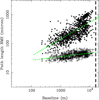
In order to discuss the characteristics of the interferometer phase fluctuations, we introduce the spatial structure function (SSF) which is a dispersion of interferometer phase as a function of a baseline length within the time interval of the whole observation duration (Thompson et al., 2001). The obtained square root of the SSF () as a function of the path length fluctuation is shown in Figures 9 and 10 for Band 7-3 and Band 8-4, respectively, using the LF DGC scans (filled circles) corrected with the WVR phase correction and HF DGC scans corrected the WVR phase correction and B2B phase referencing (plus signs). In general, the SSFs at the ALMA site show a turnover at baselines around 1 km, at which the power-law becomes shallower at longer baselines (Matsushita et al., 2017). In order to evaluate the phase stability of ALMA’s maximum baseline size (16 km), we fitted with a power-law function consisting of two components below and above the aforementioned turnover baseline. The fitted power-law functions are drawn with the dotted lines in Figures 9 and 10. The square roots of the SSFs for the shorter baseline range have the power of 0.4–0.7 and the turnover baseline of 1–3 km before B2B phase referencing (the filled circles in Figures 9 and 10), roughly consistent with the values reported in Matsushita et al. (2017).
After B2B phase referencing, the SSFs of the HF DGC scans decrease and are much less dependent on the baseline (the cross marks in Figures 9 and 10). The evaluated 16 km baseline phase RMS after B2B phase referencing are listed in Table 5. If the corrected DGC phases are a proxy for the correction achievable for the target, then we would expect that the target phase RMS would be reduced to the same level. We imaged the HF DGC source to obtain the image coherence as listed in Table 5. Phase correction at 289 GHz achieved a high image coherence of 99% and 97% for the Band 7-3(1) and 7-3(2) experiments, respectively. At 405 GHz, the DGC source image coherence is 95% and 88% for Bands 8-4(1) and 8-4(2), respectively.
In the Band 7-3 experiments, the path length fluctuations with a 16 km baseline are 27 and 57 m rms (corresponding to the phase RMS of 0.16 and 0.35 radians at 289 GHz) at Band 7-3(1) and Band 7-3(2), respectively. These values correspond to the coherence factor of 99% and 94%, consistent with the image coherence of the DGC source. In the case of Band 8-4, the path length fluctuations with a 16 km baseline are 42 and 62 m rms (corresponding to the phase rms of 0.35 and 0.53 rad at 405 GHz), so that the coherence factor is 94% and 87% at Band 8-4(1) and Band 8-4(2), respectively, which is also consistent with the image coherence. Indeed, this is as one would expect given that the residual phases after phase correction are all that should remain for the visibility data and thus remain when creating the images. The SSFs and coherence factors of the phase-corrected HF DGC source on a 16 km baseline are also listed in Table 5.
If we require an image coherence greater than 70%, the phase stability should be higher than 0.84 rad. This implies that the path length fluctuations should be smaller than 138 and 99 m RMS at the frequencies of 289 and 405 GHz, respectively. The Band 7-3(1) experiment shows that the SSF of the HF DGC source decreases to 27 m RMS in path length after B2B phase referencing. This indicates to us that if such a low path length is achievable, in similar observing conditions B2B phase referencing using ALMA long baselines at Band 9 (650 GHz) and Band 10 (950 GHz) could have achieved image coherence values of 93% and 87%, respectively, if using a phase calibrator with a small separation angle of .
6.2 Dependency of the image coherence on the switching cycle time
The residual atmospheric phase noise after phase referencing is , where is an equivalent baseline length of the phase SSF after phase referencing, is the velocity of the atmosphere at the height of the turbulent layer, and is the geometrical distance between the lines of sight to the target and the phase calibrator at the altitude of the turbulent layer (Holdaway & D’Addario, 2004). Assuming that the altitude of the turbulent layer is 500 m and is 6 m s-1 at the ALMA site (Robson et al., 2001), as well as a horizontal separation angle between the target and calibrator of at an elevation angle of , then an equivalent baseline length is , such that the dominant factor is the switching cycle time. With a shorter switching cycle time, it is clear that the residual phase is much lower given that the equivalent baseline length is obviously shorter. Furthermore, the SSF in the baseline regime 1–2 km increases with a power of (Matsushita et al., 2017); thus, an increase in could noticeably increase the residual atmospheric phase noise after the phase correction.
The baseline vector error affects the visibility phase after phase referencing as (see Section 5.3), so that the image quality is also affected by the separation angle. In the present study, we arranged the fixed target–phase calibrator pair with a small separation angle (), which might not happen often: Asaki et al. (2020) report that the expected mean separation angle to find a suitable B2B phase referencing calibrator in Bands 3 to 7, to correct a science target observed in Bands 7 to 10, is –. Crucially, it is important that the phase calibrator is close on the sky as is explored further in Maud, L. T. et al. (in preparation).
Since we adopted the fixed switching cycle time of 20 s in the SBs, we here demonstrate a 60 s switching cycle time by flagging the last two scans in every three continuous phase calibrator scans in the early stage of the data reduction. The Band 8-4 image coherence of the target was degraded to 84% for Band 8-4(1) and 68% for Band 8-4(2) with the 60 s switching cycle time, while the Band 7-3 image coherence values were maintained to 90%. The image coherence of the target and DGC source with the 60 s switching cycle time are listed in Table 5.
The SSF and corresponding coherence factor at 16 km using the DGC visibility data are also listed in Table 5. The phase RMS at 16 km baseline and using a 60 s switching cycle time are 0.25 and 0.36 rad for Band 7-3(1) and Band 7-3(2), respectively, and 0.55 and 0.85 rad for Band 8-4(1) and Band 8-4(2) respectively. The values are more consistent with the lower values of the previously mentioned 2-minute phase stability (listed in Table 3). This suggests that the 2-minute phase stability is a convenient check parameter that can be used to roughly estimate the image quality of a long-baseline observation, provided that a 60 s switching cycle time and close phase calibrator are used. As mentioned in Section 5.1, the Band 8-4(2) experiment has a rather worse phase stability compared to the other experiments: the 2-minute phase stability reaches up to 1.62 rad during the middle of the Band 8-4(2) experiments, while the other experiments have the 2-minute phase stability below 1 rad. Note that only the Band 8-4(2) experiment shows an additional 14% degradation in the image coherence compared to that with the 20 s switching cycle time, while the other experiments have only 4%–5% degradations. Thus, it is recommended for ALMA long-baseline observations that the go/no-go phase stability criterion ( 1 radian) should be strictly kept if using s switching cycle time (e.g. the 72 s switching cycle time has been used for long-baseline user observations since ALMA opened the long baseline capability in Cycle 4), while for the 20 s switching cycle time we can relax the requirement to 1–2 rad. In HF-LBC-2017, the B2B phase referencing image performance dependency on the switching cycle time was investigated in another series of experiments, which are detailed in Maud, L. T. et al. (in preparation).
The image coherence degradation as a function of the switching cycle time can be also verified using a temporal structure function (TSF) of the phase calibrator, which is defined by , where is an interferometer phase of the phase calibrator with a baseline at time . The TSF expresses the stability of the phase difference between two consecutive phase calibrator scans temporally separated by a switching cycle time. The TSF is computed for the phase calibrator at the LF and then scaled by the LF/HF frequency ratio to derive values for the HF. We evaluate the TSF for the baselines between the reference antenna and the outermost antennas (the upper quartile). For all the cases except for Band 8-4(2) with the 60 s switching cycle time, the TSFs are smaller than 1.5 rad. The TSF at Band 8-4(2) with the 60 s switching cycle time is rad when the significant image coherence degradation happens. The TSFs with the switching cycle times of 20 s and 60 s are listed in Table 5. Here, let us simplify the residual atmospheric phase error by ignoring the separation angle in this case, that is, . Since is a power-law function with a typical power of 0.6 for km, the residual atmospheric phase fluctuation of the target is expressed by . For , the TSF can be translated to the SSF as (Asaki et al., 1996). As a result, the phase RMS of the target after phase referencing is . If the TSF is 1.80 rad in this simplified case, the residual atmospheric phase fluctuation is 0.84 rad, and thus we can obtain the image coherence of 70%. In the case that the separation angle is too wide to be ignored (for example, wider than a few degrees), the requirement for the TSF is more severe, so that the criterion for the TSF would be rad with a given switching cycle time.
6.3 Target On-source Time Efficiency
If a phase calibrator is very frequently observed at HF in order to mitigate the atmospheric phase fluctuations, overheads of such observations are considerably higher than standard ALMA observations, and the effective on-source time for the target can be a small fraction of the total. For example, in the cases of our second-epoch experiments, the target on-source time is 12–13 min out of a total observation time of 1–1.5 hr, and thus the efficiency was only 15%. One of the measures to improve the on-source time efficiency is to lengthen the switching cycle time. If the 2-minute phase stability is rad, a 60 s switching cycle time can be employed (see Section 6.2), in which case the on-source efficiency will increase to 26% for the same observing time as that in Band 7-3(2).
If rather unstable weather conditions necessitate s switching cycle times, another strategy is to reduce the number of the DGC blocks. Our experimental SBs specifically included a larger number of DGC blocks in order to verify the DGC solution stability. As described in Section 5.2, the solutions are stable with the long-term time variations that can be corrected. In the case that the DGC blocks are inserted only at the beginning and end of the SBs, the on-source time efficiency is improved to 25% in Band 7-3(2). If we adopt the 60 s switching cycle time simultaneously, the on-source time efficiency is improved to 39% in Band 7-3(2).
If a phase calibrator is bright enough, it would be possible to obtain a high enough S/N in a short scan at LF, so that the phase calibrator scan length can be reduced and, instead, the target scan length can be extended. In the case of narrow-bandwidth observations for millimeter/submillimeter molecular lines with a high velocity resolution, bandwidth switching to widen the bandwidth only for the phase calibrator frequency settings would be useful to raise the S/N. The combination of the bandwidth switching and B2B phase referencing techniques would provide the highest-possible S/N for the LF phase calibrator and thus could notably improve the target on-source time. Maintaining high image quality can be done at the expense of observing efficiency, and the amount of trade-off depends on the observing conditions and scientific goals.
7 Summary
ALMA HF long-baseline experiments were conducted by adopting B2B phase referencing with a 20 s switching cycle time in order to demonstrate the ALMA high angular resolution image capability in Bands 7 and 8. In the series of experiments, we observed the target J2228–0753 paired with a phase calibrator J2229–0832 separated by . We also observed J22531608 as the DGC source to remove the instrumental phase offset difference between the HF and LF Band receivers.
The DGC solutions are temporally stable for the receiver pairs of Band 7-3 and Band 8-4 for an hour with the phase RMS of after the correction of a linear trend. For Bands 7-3 and 8-4, the DGC solutions are so stable that the two DGC blocks are enough to insert at the beginning and end of an observation lasting hr.
We achieved an angular resolution of mas at 405 GHz for the target using the maximum array configuration with 16 km baselines. We obtained high image coherence above 98% and 88% at 289 GHz and 405 GHz, respectively. One of the experiments indicates a residual path length fluctuation of 27 m RMS after B2B phase referencing, almost independent of baseline length, which would have met the requirements to achieve 70% image coherence in Bands 9 and 10 using a phase calibrator with the separation angle of . The measured astrometric positions of the target are consistent with those in the ALMA calibrator source catalogue and the VLBA calibrator source list to within 0.4 mas. Because the separation angle between the target and phase calibrator was so small, that B2B phase referencing effectively reduced the phase error due to the baseline vector uncertainties, as well as the atmospheric phase fluctuations.
We compared the image coherence achieved using the switching cycle times of 20 and 60 s, respectively. At 289 GHz, the image coherence did not significantly degrade, while at 405 GHz the image coherence decreased to 6884%. Observations that impose the condition that the 2-minute phase stability is rad satisfy the requirement that the image coherence is 70% when using 60 s switching cycle times. At higher frequencies, shorter switching cycle times will likely allow maintaining the coherence even if the 2-minute phase stability exceeds 1 rad.
References
- ALMA Partnership et al. (2015a) ALMA Partnership, Fomalont, E. B., Vlahakis, C., et al. 2015a, ApJ, 808, L1, doi: 10.1088/2041-8205/808/1/L1
- ALMA Partnership et al. (2015b) ALMA Partnership, Brogan, C. L., Pérez, L. M., et al. 2015b, ApJ, 808, L3, doi: 10.1088/2041-8205/808/1/L3
- ALMA Partnership et al. (2015c) ALMA Partnership, Vlahakis, C., Hunter, T. R., et al. 2015c, ApJ, 808, L4, doi: 10.1088/2041-8205/808/1/L4
- ALMA Partnership et al. (2015d) ALMA Partnership, Hunter, T. R., Kneissl, R., et al. 2015d, ApJ, 808, L2, doi: 10.1088/2041-8205/808/1/L2
- Andrews et al. (2016) Andrews, S. M., Wilner, D. J., Zhu, Z., et al. 2016, ApJ, 820, L40, doi: 10.3847/2041-8205/820/2/L40
- Asaki et al. (1996) Asaki, Y., Saito, M., Kawabe, R., Morita, K.-I., & Sasao, T. 1996, RaSc, 31, 1615, doi: 10.1029/96RS02629
- Asaki et al. (1998) Asaki, Y., Shibata, K. M., Kawabe, R., et al. 1998, Radio Science, 33, 1297, doi: 10.1029/98RS01607
- Asaki et al. (2007) Asaki, Y., Sudou, H., Kono, Y., et al. 2007, PASJ, 59, 397, doi: 10.1093/pasj/59.2.397
- Asaki et al. (2016) Asaki, Y., Matsushita, S., Fomalont, E. B., et al. 2016, 2016SPIE 9906, 99065U, doi: 10.1117/12.2232301
- Asaki et al. (2020) Asaki, Y., Maud, L. T., Fomalont, E. B., et al. 2020, ApJS, 247, 23, doi: 10.3847/1538-4365/ab6b20
- Bachiller & Cernicharo (2008) Bachiller, R., & Cernicharo, R. E. 2008, Science with the Atacama Large Millimeter Array: A New Era for Astrophysics, Berlin Heidelberg New York: Springer, Dordrecht
- Beasley & Conway (1995) Beasley, A. J., & Conway, J. E. 1995, 1995ASPC 82, 82, 327
- Brogan et al. (2018) Brogan, C. L., Hunter, T. R., & Fomalont, E. B. 2018, arXiv e-prints, arXiv:1805.05266. https://arxiv.org/abs/1805.05266
- Carilli & Holdaway (1999) Carilli, C. L., & Holdaway, M. A. 1999, RaSc, 34, 817
- Cornwell & Wilkinson (1981) Cornwell, T. J., & Wilkinson, P. N. 1981, MNRAS, 196, 1067, doi: 10.1093/mnras/196.4.1067
- Dodson et al. (2014) Dodson, R., Rioja, M. J., Jung, T.-H., et al. 2014, AJ, 148, 97, doi: 10.1088/0004-6256/148/5/97
- Han et al. (2013) Han, S.-T., Lee, J.-W., Kang, J., et al. 2013, PASP, 125, 539, doi: 10.1086/671125
- Hardcastle & Worrall (2000) Hardcastle, M. J., & Worrall, D. M. 2000, MNRAS, 314, 359, doi: 10.1046/j.1365-8711.2000.03393.x
- Holdaway (1992) Holdaway, M. A. 1992, MMA Memo 84. http://library.nrao.edu/alma.shtml
- Holdaway (2001) —. 2001, ALMA Memo 403. http://library.nrao.edu/alma.shtml
- Holdaway & D’Addario (2004) Holdaway, M. A., & D’Addario, L. 2004, ALMA Memo 523. http://library.nrao.edu/alma.shtml
- Hunter et al. (2016) Hunter, T. R., Lucas, R., Broguiére, D., et al. 2016, 2016SPIE 9914, 99142L, doi: 10.1117/12.2232585
- Isella et al. (2019) Isella, A., Benisty, M., Teague, R., et al. 2019, ApJ, 879, L25, doi: 10.3847/2041-8213/ab2a12
- Kervella et al. (2018) Kervella, P., Decin, L., Richards, A. M. S., et al. 2018, A&A, 609, A67, doi: 10.1051/0004-6361/201731761
- Matsushita et al. (2012) Matsushita, S., Morita, K.-I., Barkarts, D., et al. 2012, 2012SPIE 8444, 84443E, doi: 10.1117/12.925872
- Matsushita et al. (2016) Matsushita, S., Asaki, Y., Fomalont, E. B., et al. 2016, 2016SPIE 9906, 99064X, doi: 10.1117/12.2231846
- Matsushita et al. (2017) Matsushita, S., Asaki, Y., Fomalont, E. B., et al. 2017, PASP, 129, 035004, doi: 10.1088/1538-3873/aa5787
- Maud et al. (2017) Maud, L. T., Tilanus, R. P. J., van Kempen, T. A., et al. 2017, A&A, 605, A121, doi: 10.1051/0004-6361/201731197
- Maud, L. T. et al. (in preparation) Maud, L. T. et al. in preparation
- McMullin et al. (2007) McMullin, J. P., Waters, B., Schiebel, D., Young, W., & Golap, K. 2007, 2007ASPC 376, 376, 127
- Nikolic et al. (2013) Nikolic, B., Bolton, R. C., Graves, S. F., Hills, R. E., & Richer, J. S. 2013, A&A, 552, A104, doi: 10.1051/0004-6361/201220987
- Nikolic et al. (2012) Nikolic, B., Graves, S. F., Bolton, R. C., & Richer, J. S. 2012, ALMA Memo 593. http://library.nrao.edu/alma.shtml
- Nyman et al. (2010) Nyman, L.-Å., Andreani, P., Hibbard, J., & Okumura, S. K. 2010, 2010SPIE 7737, 77370G, doi: 10.1117/12.858023
- O’Gorman et al. (2015) O’Gorman, E., Harper, G. M., Brown, A., et al. 2015, A&A, 580, A101, doi: 10.1051/0004-6361/201526136
- Pérez et al. (2010) Pérez, L. M., Lamb, J. W., Woody, D. P., et al. 2010, ApJ, 724, 493, doi: 10.1088/0004-637X/724/1/493
- Remijan et al. (2020) Remijan, A., Biggs, A., Cortes, P., et al. 2020, ALMA Technical Handbook. https://almascience.nrao.edu/documents-and-tools/cycle8/alma-technical-handbook
- Rioja et al. (2014) Rioja, M. J., Dodson, R., Jung, T., et al. 2014, AJ, 148, 84, doi: 10.1088/0004-6256/148/5/84
- Robson et al. (2001) Robson, Y., Hills, R., Richer, J., et al. 2001, ALMA Memo 345. http://library.nrao.edu/alma.shtml
- Schwab (1980) Schwab, F. R. 1980, SPIE1980 231, 958828, doi: 10.1117/12.958828
- Shillue et al. (2012) Shillue, B., Grammer, W., Jacques, C., et al. 2012, 2012SPIE 8452, 845216, doi: 10.1117/12.927174
- Takahashi et al. (2019) Takahashi, S., Machida, M. N., Tomisaka, K., et al. 2019, ApJ, 872, 70, doi: 10.3847/1538-4357/aaf6ed
- Thompson et al. (2001) Thompson, A. R., Moran, J. M., & Swenson, George W., J. 2001, Interferometry and Synthesis in Radio Astronomy, 2nd Edition (A Wiley-Interscience Publication, John Wiley & Sons, Inc.)
- Tsukagoshi et al. (2019) Tsukagoshi, T., Muto, T., Nomura, H., et al. 2019, ApJ, 878, L8, doi: 10.3847/2041-8213/ab224c
- Zauderer et al. (2016) Zauderer, B. A., Bolatto, A. D., Vogel, S. N., et al. 2016, AJ, 151, 18, doi: 10.3847/0004-6256/151/1/18


|
 |
 |


|


|
 |
 |
 |
 |
 |
 |

|


|
| Date | Experiment | Time Range | Maximum | Target | Calibrator | Target On-source | Execution Block |
| Code | (UT) | Unprojected | LO1 Freq. | LO1 Freq. | Duration | (uid://A002/) | |
| Baseline Length (km) | (GHz) | (GHz) | (s) | ||||
| First Epoch | |||||||
| 2017 Oct 9 | Band 8-4(1) | 03:09 04:09 | 16.20 | 405aaThe LO1 frequency is in Band 8. | 135bbThe LO1 frequency is in Band 4. | 341 | Xc5802b/X5bb3 |
| 2017 Oct 10 | Band 7-3(1) | 03:02 03:51 | 16.20 | 289ccThe LO1 frequency is in Band 7. | 96ddThe LO1 frequency is in Band 3. | 355 | Xc59134/Xd47 |
| Second Epoch | |||||||
| 2017 Nov 2 | Band 7-3(2) | 00:57 02:21 | 13.89 | 289ccThe LO1 frequency is in Band 7. | 96ddThe LO1 frequency is in Band 3. | 411 | Xc65717/X56f |
| 2017 Nov 3 | Band 8-4(2) | 01:56 03:08 | 13.89 | 405aaThe LO1 frequency is in Band 8. | 135bbThe LO1 frequency is in Band 4. | 366 | Xc660ef/X8e0 |
| Source Name | Type | R.A. | Decl. | Separation Angle | Flux Density |
|---|---|---|---|---|---|
| (J2000) | (J2000) | from the Target | in Band 3 | ||
| (deg) | (Jy) | ||||
| J22280753 | Target | aaALMA calibrator source catalogue at 91.5 GHz on 2016 October 16. | |||
| J22290832 | Calibrator | bbALMA calibrator source catalogue at 91.5 GHz on 2017 May 5 | |||
| J22531608 | DGC source | ccALMA calibrator source catalogue at 91.5 GHz on 2017 October 22 |
| Experiment | PWV | 2-minute Phase StabilityaaAveraged phase RMS for 20% longer baselines of the HF DGC scans in a single DGC block with the time interval of 2 minutes. The minimum and maximum values are listed. | Wind Speed | Wind Direction |
|---|---|---|---|---|
| Code | (mm) | (rad)bbThe representative frequency is 289 and 405 GHz for Bands 7-3 and 8-4, respectively. | (m s-1) | (deg) |
| Band 7-3(1) | 0.48 | 0.41–0.82 | 4.2 | 305 |
| Band 7-3(2) | 0.78 | 0.40–0.58 | 5.3 | 318 |
| Band 8-4(1) | 0.77 | 0.64–0.84 | 8.1 | 314 |
| Band 8-4(2) | 0.59 | 0.67–1.62 | 4.8 | 320 |
| Experiment | Beam Size (mas) | Peak Flux Density | Peak Flux Density |
|---|---|---|---|
| Code | (Position angle (deg)) | (Image Rms Noise) | (Phase Self-alibrated) |
| (mJy beam-1) | (Image Rms Noise) | ||
| (mJy beam-1) | |||
| Band 7-3(1) | () | 45.32 (0.11) | 46.85 (0.05) |
| Band 7-3(2) | () | 44.82 (0.15) | 50.00 (0.07) |
| Band 8-4(1) | () | 34.63 (0.23) | 37.90 (0.20) |
| Band 8-4(2) | () | 31.37 (0.22) | 38.84 (0.18) |
| Switching | Target | Phase-corrected HF DGC Scan | Phase | ||||
| Experiment | Cycle | Image | SSFbbSSF: spatial structure function. See Sections 6.1 and 6.2 in detail. (16 km) | SSFbbSSF: spatial structure function. See Sections 6.1 and 6.2 in detail. (16 km) | Coherence FactorccCoherence factor is calculated by , where is the phase RMS with a 16 km baseline. See Sections 1, 6.1, and 6.2 in detail. | Image | Calibrator |
| Code | Time (s) | CoherenceaaImage coherence is the ratio of the image peak flux density compared to the true value. See Sections 5.3, 6.1, and 6.2 in detail. (%) | (m RMS) | (rad) | (16 km) (%) | CoherenceaaImage coherence is the ratio of the image peak flux density compared to the true value. See Sections 5.3, 6.1, and 6.2 in detail. (%) | TSFddTSF: temporal structure function. See Section 6.2 in detail. (rad) |
| Band 7-3(1) | 20 | 97 | 27 | 0.16 | 99 | 99 | 0.48 |
| 60 | 92 | 40 | 0.25 | 97 | 96 | 0.93 | |
| Band 7-3(2) | 20 | 93 | 57 | 0.35 | 94 | 97 | 0.57 |
| 60 | 89 | 59 | 0.36 | 94 | 94 | 1.05 | |
| Band 8-4(1) | 20 | 87 | 42 | 0.36 | 94 | 95 | 0.75 |
| 60 | 84 | 65 | 0.55 | 86 | 91 | 1.23 | |
| Band 8-4(2) | 20 | 82 | 62 | 0.53 | 87 | 88 | 1.47 |
| 60 | 68 | 100 | 0.85 | 70 | 74 | 2.52 | |
| Experiment Code | R.A. ( Error) | Decl. ( Error) |
|---|---|---|
| (J2000) | (J2000) | |
| Band 7-3(1) | (0.02 mas) | (0.02 mas) |
| Band 7-3(2) | (0.04 mas) | (0.03 mas) |
| Band 8-4(1) | (0.04 mas) | (0.03 mas) |
| Band 8-4(2) | (0.06 mas) | (0.04 mas) |