Algorithmic Regularization in Model-free Overparametrized Asymmetric Matrix Factorization

Liwei Jiang Yudong Chen Lijun Ding School of Operations Research and Information Engineering, Cornell University. Ithaca, NY 14850, USA; [email protected] of Computer Sciences, University of Wisconsin-Madison. Madison, WI 53706, USA; [email protected] Institute for Discovery, University of Wisconsin-Madison, Madison, WI 53706, USA; [email protected]

Abstract

We study the asymmetric matrix factorization problem under a natural nonconvex formulation with arbitrary overparametrization. The model-free setting is considered, with minimal assumption on the rank or singular values of the observed matrix, where the global optima provably overfit. We show that vanilla gradient descent with small random initialization sequentially recovers the principal components of the observed matrix. Consequently, when equipped with proper early stopping, gradient descent produces the best low-rank approximation of the observed matrix without explicit regularization. We provide a sharp characterization of the relationship between the approximation error, iteration complexity, initialization size and stepsize. Our complexity bound is almost dimension-free and depends logarithmically on the approximation error, with significantly more lenient requirements on the stepsize and initialization compared to prior work. Our theoretical results provide accurate prediction for the behavior gradient descent, showing good agreement with numerical experiments.

1 Introduction

Let $X\in\mathbb{R}^{m\times n}$ be an arbitrary given matrix. In this paper, we study the following nonconvex objective function for asymmetric matrix factorization

\displaystyle f(F,G):=\frac{1}{2}\|FG^{\top}-X\|_{{\tiny\text{F}}}^{2}\quad

(

\mathcal{M}

)

and the associated vanilla gradient descent dynamic:

\displaystyle\text{initialize}\;(F_{0},G_{0});\;\;\text{run iteration}\;(F_{t+1},G_{t+1})=(F_{t},G_{t})-\eta\nabla f(F_{t},G_{t}),

(

\mathcal{GD}

\mathcal{M}

)

where $(F,G)\in\mathbb{R}^{m\times k}\times\mathbb{R}^{n\times k}$ are the factor variables, $k\geq 1$ is a user-specified rank parameter, $\eta>0$ is the stepsize, and $\nabla f(F,G)=((FG^{\top}-X)G,(FG^{\top}-X)^{\top}F).$

In many statistical and machine learning settings [FYY20], the observed matrix $X$ takes the form $X=X_{\natural}+E,$ where $X_{\natural}$ is an unknown low-rank matrix to be estimated, and $E$ is the additive error/noise. Gradient descent applied to the objective ( $\mathcal{M}$ ) is a natural approach for computing an estimate of $X_{\natural}$ . Such an estimate can in turn be used as an approximate solution in more complicated nonconvex matrix estimation problems, such as matrix sensing [RFP10], matrix completion [CT10] and even nonlinear problems like the Single Index Model [FYY20]. In fact, the gradient descent procedure ( $\mathcal{GD}$ - $\mathcal{M}$ ) is often used, explicitly or implicitly, as a subroutine in more sophisticated algorithms for these problems. As such, characterizing the dynamics of ( $\mathcal{GD}$ - $\mathcal{M}$ ) provides deep intuition for more general problems and is considered an important first step for understanding various aspects of (linear) neural networks [DHL18, YD21].

Despite the apparent simplicity of the dynamic ( $\mathcal{GD}$ - $\mathcal{M}$ ), our understanding of its behavior remains limited, especially for general settings of $X$ and $k$ . Results in existing work often only apply to symmetric, exactly low-rank matrices $X$ or specific choices of $k$ . Many of them impose strong assumption on the initialization $(F_{0},G_{0})$ , only provides asymptotic analysis, or has order-wise suboptimal error and iteration complexity bounds. We discuss these existing results and the associated challenges in greater details later.

Of particular interest is the overparametrization regime, which is common in modern machine learning paradigms [HCB⁺19, KBZ⁺20, TL19]. In the context of the objective ( $\mathcal{M}$ ), overparametrization means choosing the rank parameter $k$ to be larger than what is statistically necessary, e.g., $k=\min\{m,n\}\gg$ rank $(X_{\natural})$ . Doing so, however, necessarily leads to overfitting in general. Indeed, with $k=\min\{m,n\}$ , any global optimum of ( $\mathcal{M}$ ) is simply (a full factorization of) $X$ itself and overfits the noise/error in $X$ , therefore failing to provide a useful estimate for $X_{\natural}$ . Moreover, as can be seen from the numerical results in Figure 1, gradient descent ( $\mathcal{GD}$ - $\mathcal{M}$ ) with random initialization asymptotically converges to such a global minimum, with a vanishing training error $\|FG^{\top}-X\|_{{\tiny\text{F}}}$ (dashed lines) but a large test error $\|FG^{\top}-X_{\natural}\|_{{\tiny\text{F}}}$ (solid lines).

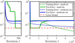
Refer to caption — Figure 1: Evolution of training error $\|F_{t}G_{t}^{\top}-X\|_{{\tiny\text{F}}}$ and testing error $\|F_{t}G_{t}^{\top}-X_{\natural}\|_{{\tiny\text{F}}}$ of ( $\mathcal{GD}$ - $\mathcal{M}$ ) with $k=200$ under the model $X=X_{\natural}+E$ , where $X_{\natural}\in\mathbb{R}^{250\times 200}$ has rank $r=5$ and $\|X_{\natural}\|_{{\tiny\text{F}}}=1$ , and the noise matrix $E$ has i.i.d. zero-mean Gaussian entries and expected operator norm $\mathbb{E}\|E\|\approx 2\times 10^{-3}$ . The green lines use small initialization ( $\|F_{0}\|_{{\tiny\text{F}}},\|G_{0}\|_{{\tiny\text{F}}}\ll\|X_{\natural}\|_{{\tiny\text{F}}}$ ), and the blue lines use moderate initialization ( $\|F_{0}\|_{{\tiny\text{F}}},\|G_{0}\|_{{\tiny\text{F}}}\asymp\|X_{\natural}\|_{{\tiny\text{F}}}$ ). The red line represents the optimal statistical error $\sqrt{r}\|E\|$ . The left panel zooms in the first 600 iterations.

A careful inspection of Figure 1, however, reveals an interesting phenomenon: gradient descent with small random initialization achieves a small (and near optimal) test error before it eventually overfits; on the other hand, this behavior is not observed with moderate initialization. We note that similar phenomena have been empirically observed in many other statistical and machine learning problems, where vanilla gradient descent coupled with small random initialization (SRI) and early stopping (ES) has good generalization performance, even with overparametrization [WGL⁺20, GMMM20, Pre98, WLZ⁺21, LMZ18, SS21]. This observation motivates us to theoretically characterize, both qualitatively and quantitatively, the behavior of gradient descent ( $\mathcal{GD}$ - $\mathcal{M}$ ) and the algorithmic regularization effect of SRI and ES.

Our results

We relate the dynamics of ( $\mathcal{GD}$ - $\mathcal{M}$ ) to the best low-rank approximations of $X$ , defined as $X_{r}=\operatornamewithlimits{argmin}_{\mathrm{rank}(Y)\leq r}\|Y-X\|_{{\tiny\text{F}}}^{2}$ for $r=1,2,\ldots$ Our main results, Theorems 4.1 and 4.2, establish the following:

The iteration ( $\mathcal{GD}$ - $\mathcal{M}$ ) with SRI sequentially approaches the principal components of $X$ , and proper ES produces the best low-rank approximation of $X$ .

Specifically, we show that for each $r\in[1,k]$ , there exists a (range of) stopping time $t$ such that ( $\mathcal{GD}$ - $\mathcal{M}$ ) terminated at iteration $t$ produces an approximate $X_{r}$ . Moreover, we provide a sharp characterization of the scaling relationship between the approximation error, iteration complexity, initialization size and stepsize. This quantitative characterization agrees well with numerical experiments.

It is known that under many statistical models where $X$ is an observed noisy version of some structured matrix $X_{\natural}$ , the matrix $X_{r}$ with an appropriate $r$ is a statistically optimal estimator of $X_{\natural}$ [Cha15, FYY20]. Our results thus imply that gradient descent with SRI and ES learns such an optimal estimate, even with overparametrization and no explicit regularization. In fact, our results are more general, applicable to any observed matrix $X$ and not tied to the existence of a ground truth $X_{\natural}$ .

We emphasize that we do not claim that vanilla gradient descent is a more efficient way for computing $X_{r}$ for a given $r$ than standard numerical procedures (e.g., via singular value decomposition). Rather, our focus is to show, rigorously and quantitatively, that overparametrized gradient descent, a common and fundamental algorithmic paradigm, has an implicit regularization effect characterized by a deep connection to the computation of best low-rank approximation.

Analysis and challenges

Our analysis elucidates the mechanism that gives rise to the algorithmic regularization effect of small initialization and early stopping: starting from a small initial $F_{0}G_{0}^{\top}$ , the singular values of the iterate $F_{t}G_{t}^{\top}$ approach those of $X$ at geometrically different rates, hence $F_{t}G_{t}^{\top}$ approximates $X_{1},X_{2},\ldots$ sequentially (we elaborate in Section 3). While the intuition is simple, a rigorous and sharp analysis is highly non-trivial, due to the following challenges:

(i) Model-free setting. Most existing work assumes that $X$ is (exactly or approximately) low-rank with a sufficiently large singular value gap $\delta$ between the $r$ -th and $(r+1)$ -th singular values of $X$ [LMZ18, ZKHC21, YD21, FYY20, SS21]. We allow for an arbitrary nonzero $\delta$ and characterize its impact on the stopping time and final error. In this setting, the “signal” $X_{r}$ may have magnitude arbitrarily close to that of the “noise” $X-X_{r}$ even in operator norm.

(ii) Asymmetry. Since the objective ( $\mathcal{M}$ ) is invariant under the rescaling $(F,G)\to(cF,c^{-1}G)$ , the magnitudes of $F$ and $G$ may be highly imbalanced, in which case the gradient has a large Lipschitz constant. This issue is well recognized to be a primary difficulty in analyzing the gradient dynamics ( $\mathcal{GD}$ - $\mathcal{M}$ ) even without overparametrization [DHL18]. Most previous works either restrict to the symmetric positive semidefinite formulation [LMZ18, ZKHC21, SS21, ZFZ21, MF21, DJC⁺21, Zha21], or add an explicit regularization term of the form $\|F^{\top}F-G^{\top}G\|_{{\tiny\text{F}}}^{2}$ [TBS⁺16, ZL16].

(iii) Trajectory analysis and cold start. As the desired $X_{r}$ is not a local minimizer of ( $\mathcal{M}$ ), our analysis is inherently trajectory-based and initialization-specific.

Random initialization leads to a cold start: the initial iterates $F_{t}G_{t}^{\top}$ are far from and nearly orthogonal to $X_{r}$ when the dimensions $(m,n)$ are large. More precisely, assuming the SVD $X_{r}=U\Sigma V^{\top}$ , one may measure the relative signal strength of $(F_{t},G_{t})$ by

\texttt{sig}(F_{t},G_{t}):=\frac{\min\{\sigma_{r}(U^{\top}F_{t}),\sigma_{r}(V^{\top}G_{t})\}}{\max\{\sigma_{1}((I-UU^{\top})F_{t}),\sigma_{1}((I-VV^{\top})G_{t})\}},

(1.1)

which is the ratio between the projections of $F_{t}$ and $G_{t}$ to the column/row space of $X$ and the projections to the complementary space. Most existing work requires $\texttt{sig}(F_{0},G_{0})$ to be larger than a universal constant [FYY20, LMZ18], which does not hold when $k,r=o(m)$ .¹¹1For $F_{0},G_{0}$ with i.i.d. standard Gaussian entries, we have w.h.p. $\texttt{sig}(F_{0},G_{0})\lesssim\frac{\sqrt{k}+\sqrt{r-1}}{|\sqrt{m-r}-\sqrt{k}|}$ for $m\asymp n$ .

(iv) General rank overparametrization. Our result holds for any choice of $k$ with $k\geq r$ . The work in [YD21, MLC21] only considers the exact-parametrization setting $k=r$ . The work [FYY20] assumes the specific choice $k=2m+2n$ ; as mentioned in the previous paragraph, the setting with a smaller $k$ involves additional challenges due to cold-start.

2 Related work

The literature on gradient descent for matrix factorization is vast; see [CC18, CLC19] for a survey. Most prior work focuses on the exact parametrization setting $k=r$ (where $r$ is the target rank or the rank of a ground truth matrix $X_{\natural}$ ) and requires an explicit regularizer $\|F^{\top}F-G^{\top}G\|_{{\tiny\text{F}}}^{2}$ . More recent work in [DJC⁺21, DHL18, FYY20, LMZ18, MLC21, MF21, SS21, YD21, ZFZ21, Zha21, ZKHC21], discussed in the last section, studies (overparametrized) matrix factorization and implicit regularization. Below we discuss recent results that are most related to ours.

The work [FYY20] considers a wide range of statistical problems with a symmetric ground truth matrix $X_{\natural}$ and shows that $X_{\natural}$ can be recovered with near optimal statistical errors using gradient descent for ( $\mathcal{M}$ ) with $FG^{\top}$ replaced by $FF^{\top}-GG^{\top}$ . While one may translate their results to the asymmetric setting via a dilation argument, doing so requires the specific rank parametrization $k=2m+2n$ . This restriction allows for a decoupling of the dynamics of different singular values, which is essential to their analysis. While this decoupled setting provides intuition for the general setting (as we elaborate in Section 3), the same analysis no longer applies for other values of $k$ , e.g., $k=2m+2n-1$ , for which the decoupling ceases to hold. Moreover, a smaller value of $k$ leads to the cold start issue, as discussed in footnote 1.

The work in [CGMR20] studies the deep matrix factorization problem. While on a high level their results deliver a message similar to our work, namely gradient descent sequentially approaches the principal components of $X$ , the technical details differ significantly. In particular, they results only apply to symmetric $X$ and guarantee recovery of the positive semidefinite part of $X$ . Their analysis relies crucially on the assumption $k=m=n$ , a specific identity initialization scheme and the resulting decoupled dynamics, which do not hold in the general setting as discussed above. A major contribution of our work lies in handling the entanglement of singular values resulted from general overparametrization, asymmetry, and random initialization.

In Section C, we provide additional discussion on related work.

3 Intuitions and the symmetric setting

In this section, we illustrate the behavior of gradient descent with small random initialization in the setting with a symmetric $X$ , and explain the challenges for generalizing to asymmetric $X$ .

Consider a simple example where $m=n=k=2$ , and $X={\rm diag}(\lambda_{1},\lambda_{2})$ is a positive semidefinite diagonal matrix that is approximately rank-1, i.e., $\lambda_{2}\leq\frac{1}{10}\lambda_{1}$ . We consider the natural symmetric objective $f(F)=\frac{1}{4}\|FF^{\top}-X\|_{{\tiny\text{F}}}^{2}$ and the associated gradient descent dynamic $F_{t+1}=F_{t}-\eta(F_{t}F_{t}^{\top}-X)F_{t}$ ,²²2This is equivalent to ( $\mathcal{GD}$ - $\mathcal{M}$ ) with initialization $F_{0}=G_{0}$ . with initialization $F_{0}=\rho\sqrt{\lambda_{1}}I$ for some small $\rho>0$ .

It is easy to see that $F_{t}$ is diagonal for all $t\geq 0$ , and the $i$ -th diagonal element of $F_{t}$ , denoted by $f_{i,t}$ , is updated as

f_{i,t+1}=f_{i,t}(1+\eta\lambda_{i}-\eta f_{i,t}^{2}),\quad i=1,2.

(3.1)

Thus, the dynamics of the two eigenvalues decouple and can be analyzed separately. In particular, simple algebra shows that (i) when $f_{1,t}<\sqrt{\frac{\lambda_{1}}{2}}$ , $f_{1,t}$ increases geometrically by a factor of $1+\eta\lambda_{1}-\eta f_{1,t}^{2}\geq 1+\frac{\eta\lambda_{1}}{2}$ , i.e., $|f_{1,t+1}|\geq(1+\frac{\eta\lambda_{1}}{2})|f_{1,t}|$ , and (ii) when $f_{1,t}\geq\sqrt{\frac{\lambda_{1}}{2}}$ , $f_{1,t}$ converges to $\sqrt{\lambda_{1}}$ geometrically with a factor of $(1-\frac{\eta\lambda_{1}}{2})$ , i.e., $|f_{1,t+1}-\sqrt{\lambda_{1}}|\leq(1-\frac{\eta\lambda_{1}}{2})|f_{1,t}-\sqrt{\lambda_{1}}|.$ In a similar fashion, $f_{2,t}$ converges to the second eigenvalue $\sqrt{\lambda_{2}}$ . It follows that the gradient descent iterate $F_{t}F_{t}^{\top}$ converges to the observed matrix $X$ as $t$ goes to infinity.

What makes a difference, however, is that $f_{2,t}$ converges at an exponentially slower rate than $f_{1,t}$ . In particular, assuming the stepsize $\eta$ is sufficiently small, we can show that $f_{2,t}$ is always nonnegative and satisfies $f_{2,t+1}\leq(1+\frac{\eta\lambda_{1}}{10})f_{2,t}$ . Note that the growth factor $1+\frac{\eta\lambda_{1}}{10}$ is smaller than $1+\frac{\eta\lambda_{1}}{2}$ , the growth factor for $f_{1,t}$ . We conclude that

With small initialization, larger eigenvalues converge (exponentially) faster.

(3.2)

Thanks to the property (3.2), the gradient descent trajectory approaches the principal components of $X$ one by one. In particular, if the initial size $\rho$ is sufficiently small, then (3.2) implies the existence of time window for $t$ during which $f_{1,t}$ is close to $\lambda_{1}$ while $f_{2,t}$ remains close to its initial value (i.e., close to $0$ ). If we terminate at a time $t$ within this window, then the gradient descent output satisfies $F_{t}F_{t}^{\top}\approx X_{1}$ . If we continue the iteration, then $f_{2,t}$ eventually grows away from $0$ and converges quickly to $\sqrt{\lambda_{2}}$ , yielding $F_{t}F_{t}^{\top}\approx X_{2}$ .

In Section C, we generalize the above argument to any $m\times m$ symmetric positive semi-definite $X$ via a diagonalization argument, which shows that $F_{t}F_{t}^{\top}$ approaches $X_{1},X_{2},X_{3},\ldots$ sequentially. However, this simple derivation breaks down for general rectangular $F_{t}$ and $X$ , since the dynamics of eigenvalues no longer decouple as in (3.1); rather, they have complicated dependence on each other, as can be seen in the proof of our main theorems. One of the main contributions of our proof is to rigorously establish the property (3.2) despite this complicated dependence.

4 Main results and analysis

In this section, we present our main theorems on the trajectory of gradient descent under small random initialization and early stopping. We also outline the analysis, deferring the full proof to the appendices.

4.1 Main theorems

Recall that $X\in\mathbb{R}^{m\times n}$ is a general rectangular matrix and denote its singular values by $\sigma_{1}\geq\cdots\geq\sigma_{\min\{m,n\}}\geq 0$ . Fix $r\in[0,\min\{k,m,n\}]$ and define the $r$ -th condition number $\kappa_{r}:=\frac{\sigma_{1}}{\sigma_{r}}$ . Suppose that the gradient descent dynamic ( $\mathcal{GD}$ - $\mathcal{M}$ ) is initialized with $(F_{0},G_{0})=\frac{\rho}{3\sqrt{m+n+k}}(\tilde{F}_{0},\tilde{G}_{0})$ , where $\rho>0$ is a size parameter and $\tilde{F}_{0}\in\mathbb{R}^{m\times k},\tilde{G}_{0}\in\mathbb{R}^{n\times k}$ have i.i.d. $N(0,\sigma_{1})$ entries. The operator norm is denoted by $\|\cdot\|$ .

Below we state two theorems under one of the following assumptions:

Assumption A.

The first $r+1$ singular values are distinct, i.e., $\sigma_{1}>\cdots>\sigma_{r}>\sigma_{r+1}$ .

Assumption B.

The $r$ -th and $(r+1)$ -th singular values are distinct, i.e., $\sigma_{r}>\sigma_{r+1}.$

Both theorems are high probability statements (w.r.t. random initialization); we refer to Theorem A.1 in the appendix for the precise value of the probability.

Our first theorem shows that under Assumption A, gradient descent with small random initialization approaches the principal components $X_{1},X_{2},\ldots,X_{r}$ sequentially.

Theorem 4.1.

Suppose that Assumption A holds and let $\underline{\delta}$ be any number in $(0,1)$ such that $\underline{\delta}\leq\min_{1\leq s\leq r}\{\frac{\sigma_{s}-\sigma_{s+1}}{\sigma_{s}}\}$ . Fix any tolerance $\epsilon\leq\frac{1}{m+n+k}$ . Then, there exist some numerical constants $c,c^{\prime}$ and a sequence of iteration indices

T^{(1)}\leq T^{(2)}\leq\ldots T^{(r)}\leq\frac{c^{\prime}}{\underline{\delta}\eta\sigma_{r}}\log\left(\frac{\kappa_{r}}{\underline{\delta}\epsilon}\right)

such that with high probability, the iterates of gradient descent ( $\mathcal{GD}$ - $\mathcal{M}$ ) with stepsize $\eta\leq c\min\{\underline{\delta},1-\underline{\delta}\}\frac{\sigma_{r}^{2}}{\sigma_{1}^{3}}$ and initialization size $\rho\leq\left(\frac{c\underline{\delta}\epsilon}{\kappa_{r}}\right)^{\frac{1}{c\underline{\delta}}}$ satisfy

\|F_{T^{(s)}}G_{T^{(s)}}^{\top}-X_{s}\|\leq\epsilon\sigma_{1},\quad\forall s=1,2,\ldots,r.

Our next, more precise theorem applies under Assumption B and shows that there is in fact a range of iterations at which gradient descent approximates $X_{r}$ . Note that the first theorem can be derived by applying the second theorem to each $r=1,2,\ldots$

Theorem 4.2.

Suppose that Assumption B holds and let $\underline{\delta}$ be any number in $(0,1)$ such that $\underline{\delta}\leq\delta:=\frac{\sigma_{r}-\sigma_{r+1}}{\sigma_{r}}$ . Fix any tolerance $\epsilon\leq\frac{1}{m+n+k}$ . The following holds with high probability for some numerical constants $c,c^{\prime}$ . Consider gradient descent ( $\mathcal{GD}$ - $\mathcal{M}$ ) with stepsize $\eta\leq c\min\{\underline{\delta},1-\underline{\delta}\}\frac{\sigma_{r}^{2}}{\sigma_{1}^{3}}$ and initialization size $\rho\leq\left(\frac{c\underline{\delta}\epsilon}{\kappa_{r}}\right)^{\frac{1}{c\underline{\delta}}}$ . Let $T=\Big{\lfloor}\frac{\log(\rho^{\frac{\underline{\delta}}{2(2-\underline{\delta})}}/\rho)}{\log(1+(1-\underline{\delta})\eta\sigma_{r})}\Big{\rfloor}$ , which is $O\left(\frac{1}{\underline{\delta}\eta\sigma_{r}}\log\left(\frac{\kappa_{r}}{\underline{\delta}\epsilon}\right)\right)$ for $\rho=\left(\frac{c\underline{\delta}\epsilon}{\kappa_{r}}\right)^{\frac{1}{c\underline{\delta}}}$ . Then, for all $t$ such that $(1-c^{\prime}\underline{\delta})T\leq t\leq T$ , we have

\|F_{t}G_{t}^{\top}-X_{r}\|\leq\epsilon\sigma_{1}.

(4.1)

We highlight that Theorem 4.2 applies to any observed matrix $X$ with a nonzero singular value gap $\delta$ ,³³3Otherwise $X_{r}$ is not uniquely defined. which can be arbitrarily small; we refer to this as the model-free setting. Moreover, Theorem 4.2 quantifies the relationship between various problem parameters: if $X$ has a relative singular value gap $\delta$ , then gradient descent with initialization size $\rho\lesssim\epsilon^{\frac{1}{\delta}}$ and early stopping at iteration $O\left(\frac{1}{\delta}\log\frac{1}{\epsilon}\right)$ outputs $X_{r}$ up to an $\epsilon$ error (we ignore logarithmic terms).

We make two remarks regarding the tightness of the above parameter dependence.

•

Final error, initialization size, and eigen gap: The final error $\epsilon$ can be made arbitrarily small as long as the initialization size $\rho$ is sufficiently small. Moreover, as verified by our numerical experiments in Section 5, the scaling $\rho\lesssim\epsilon^{\frac{1}{\delta}}$ predicted by Theorem 4.2 is quite accurate.
•

Iteration complexity and stepsize: The number of iterations needed for an $\epsilon$ error scales as $\log(1/\epsilon)$ , which is akin to a geometric/linear convergence rate. Moreover, our stepsize and iteration complexity are independent of the dimension $m,n$ (up to log factors), both of which improve upon existing results in [YD21], which requires a significantly smaller stepsize and hence an iteration complexity proportional to $(m+n)^{2}$ . Again, our dimension-independent scaling agrees well with the numerical results in Section 5.

4.2 Proof Sketch for Theorem 4.2

We sketch the main ideas for proving Theorem 4.2 and discuss our main technical innovations. Our proof is inspired by the work [YD21], which studies the setting with low-rank $X$ and exact parametrization $k=r=\text{rank}(X)$ .

We start by simplifying the problem using the singular value decomposition (SVD) $X=\Phi\Sigma_{X}\Psi^{\top}$ of $X$ , where $\Phi\in\mathbb{R}^{m\times m},\Sigma_{X}\in\mathbb{R}^{m\times n}$ and $\Psi\in\mathbb{R}^{n\times n}$ . By replacing $F$ , $G$ with $\Phi^{\top}F$ , $\Psi^{\top}G$ , respectively, we may assume without loss of generality that $X$ is diagonal. The distribution of the initial iterate $(F_{0},G_{0})$ remains the same thanks to the rotational invariance of Gaussian. Hence, the gradient descent update ( $\mathcal{GD}$ - $\mathcal{M}$ ) becomes

F_{+}=F+\eta(\Sigma_{X}-FG^{\top})G,\quad\text{and}\quad G_{+}=G+\eta(\Sigma_{X}-FG^{\top})^{\top}F,

(4.2)

where the subscript $+$ indicates the next iterate and will be used throughout the rest of the paper. Let $U$ be the upper $r\times k$ submatrix of $F$ and $J$ be the lower $(m-r)\times k$ submatrix of $F$ . Similarly, let $V$ be the upper $r\times k$ submatrix of $G$ and $K$ be the lower $(n-r)\times k$ submatrix of $G$ . Also let $\Sigma={\rm diag}(\sigma_{1},\ldots,\sigma_{r})$ be the upper left $r\times r$ submatrix of and $\tilde{\Sigma}\in\mathbb{R}^{(m-r)\times(n-r)}$ be a diagonal matrix with $\sigma_{r+1},\ldots,\sigma_{\min\{m,n\}}$ on the diagonal. The gradient descent update (4.2) induces the following update for the “signal” matrices $U,V$ and the “error” matrices $J,K$ :

\displaystyle\begin{cases}U^{+}=U+\eta\Sigma V-\eta U(V^{\top}V+K^{\top}K)\\ V^{+}=V+\eta\Sigma U-\eta V(U^{\top}U+J^{\top}J)\\ J^{+}=J+\eta\tilde{\Sigma}K-\eta J(V^{\top}V+K^{\top}K)\\ K^{+}=K+\eta\tilde{\Sigma}^{\top}J-\eta K(U^{\top}U+J^{\top}J).\end{cases}

(4.3)

We may bound the difference $FG^{\top}-X_{r}$ as the following:

\displaystyle\|FG^{\top}-X_{r}\|\leq\|UV^{\top}-\Sigma\|+\|UK^{\top}\|+\|JV^{\top}\|+\|JK^{\top}\|.

Hence, it suffices to show that the signal term $UV^{\top}$ converges to $\Sigma$ and the error term $(J,K)$ remains small. To account for the potential imbalance of $U$ and $V$ , we introduce the following quantities using the symmetrization idea in [YD21]:

\displaystyle A=\frac{U+V}{2},\;B=\frac{U-V}{2},\;P=\Sigma-AA^{\top}+BB^{\top},\;\text{and}\;Q=AB^{\top}-BA^{\top}.

(4.4)

(Similarly define $A_{t},B_{t},P_{t},Q_{t}$ based on the $t$ -th iterates.) Here $A$ is the symmetrized part of the signal terms $U,V$ , and $B$ represents the imbalance between them. Since $\Sigma-UV^{\top}=P+Q$ , the quantities $P$ and $Q$ capture how far the signal term is from the true signal $\Sigma$ . Let $T$ be iteration index defined as in Theorem 4.2. Our proof studies three phases of lengths $T_{1},T_{2},T_{3}$ within these $T$ iterations, where $T_{1}+T_{2}+T_{3}\leq T$ . The proof consists of three steps:

•

Step 1. We use induction on $t$ to show that the error term $(J_{t},K_{t})$ and the imbalance term $B_{t}$ remain small throughout the $T$ iterations.
•

Step 2. We characterize the evolution of the smallest singular value $\sigma_{r}(A_{t})$ . After the first $T_{1}$ iteration, the value $\sigma_{r}(A_{t})$ dominates the errors. Then, with $T_{2}$ more iterations, $\sigma_{r}(A_{t})$ grows above the threshold $0.8\sqrt{\sigma_{r}}$ , in which case signal term $UV^{\top}$ has magnitude close to that of the true signal $\Sigma_{r}$ .
•

Step 3. After $\sigma_{r}(A_{t})$ becomes sufficiently large, we show that $\|P_{t}\|$ decreases geometrically. After $T_{3}$ more iterations, $\|P_{t}\|$ has the same magnitude as the error terms $J_{t},K_{t}$ . Theorem 4.2 then follows by bounding $\|F_{t}G_{t}^{\top}-X_{r}\|$ in terms of $P_{t},Q_{t},J_{t},K_{t}$ .

Our analysis of $P_{t}$ and $B_{t}$ departs from that in [YD21], which requires the stepsize $\eta$ to depend on both problem dimension and initialization size, resulting in an iteration complexity that has polynomial dependence on the dimension. The better dependence in our Theorem 4.2 is achieved using the following new techniques:

1.

Unlike [YD21] which bounds ${B_{t}},{J_{t}},{K_{t}}$ by quantities independent of $t$ , we control them using geometrically increasing series, which are tighter and more accurately capture the dynamics of ${B_{t}},{J_{t}},{K_{t}}$ across $t$ .
2.

Our analysis decouples the choices of the stepsize $\eta$ and initialization size $\rho$ , allowing them to be independent. We do so by making the crucial observation that the desired lower bound on $\lambda_{r}(P_{t})$ only depends on $\sigma_{r}$ and the singular value gap $\delta$ . As a result, we can take a very small initialization size $\rho$ (in both theory and experiments), since the iteration complexity depends only logarithmically on $\rho$ . In contrast, the desired lower bound on $\lambda_{r}(P_{t})$ in [YD21] depends on initialization size $\rho$ , and in turn their stepsize $\eta$ have more stringent dependence on $\rho$ .
3.

The analysis in [YD21] cannot be easily generalized to the overparametrized setting, since in this case the error terms $\|J_{t}\|,\|K_{t}\|$ no longer decay geometrically when they are within a small neighborhood of zero—to our best knowledge, tightly characterizing this local convergence behavior in the overparametrized setting remains an open problem. We circumvent this difficulty by using a smaller initialization size $\rho$ , which is made possible by the tighter analysis outlined in the last bullet point.

5 Experiments

We present numerical experiments that corroborate our theoretical findings on gradient descent with small initialization and early stopping. In Section 5.1, we provide numerical results that demonstrate the dynamics and algorithmic regularization of gradient descent. In Section 5.2, we numerically verify our theoretical prediction on the scaling relationship between the initialization size, stepsize, iteration complexity and final error.

5.1 Dynamics of gradient descent

We generate a random rank- $10$ matrix $X\in\mathbb{R}^{m\times n}$ with $m=250,n=200$ and $\|X\|_{{\tiny\text{F}}}=1$ , and run gradient descent ( $\mathcal{GD}$ - $\mathcal{M}$ ) with initialization size $\rho=10^{-6}$ , stepsize $\eta=0.5$ and rank parameter $k=200$ . As shown in Figure 2a, the top singular values $\sigma_{i}(F_{t}G_{t}^{\top})$ of the iterate grow towards those of $X$ sequentially at geometrically different rates. Consequently, for each $r=1,2,\ldots$ , the iterate $F_{t}G_{t}^{\top}$ is close to the best rank- $r$ approximation $X_{r}$ when $\sigma_{i}(F_{t}G_{t}^{\top})\approx\sigma_{i}(X),1\leq i\leq r$ and $\sigma_{i}(F_{t}G_{t}^{\top})\approx 0,i\geq r+1$ ; early stopping of gradient descent at this time outputs $X_{r}$ .

In Figure 2b, we compare the convergence rates of gradient descent with small ( $\rho\in\{10^{-2},10^{-4},10^{-6}\}$ ) and moderate ( $\rho=1$ ) initialization sizes. We see that using a small $\rho$ results in fast convergence to a small error level; moreover, the convergence rate is geometric-like (before saturation), which is consistent with the $\log(1/\epsilon)$ iteration complexity predicted by Theorem 4.2. Therefore, compared to moderate initialization, small initialization has both computational benefit (in terms of iteration complexity) and a statistical regularization effect (when coupled with early stopping, as demonstrated in Figure 1).

5.2 Parameter dependence

Theorem 4.2 predicts that if $X$ has relative singular value gap $\delta=\frac{\sigma_{r}-\sigma_{r+1}}{\sigma_{r}}$ , then gradient descent outputs $X_{r}$ with a relative error $\|F_{t}G_{t}^{\top}-X_{r}\|_{{\tiny\text{F}}}/\|X_{r}\|_{{\tiny\text{F}}}=\epsilon$ in $T_{0}=O\left(\frac{1}{\delta}\log\frac{1}{\epsilon}\right)$ iterations when using an initialization size $\rho\asymp\epsilon^{\frac{1}{\delta}}$ and a stepsize nearly independent of the dimension of $X$ . We numerically verify these scaling relationships.

In all experiments, we fix $r=3$ , stepsize $\eta=0.25$ and rank parametrization $k=10$ , and generate a matrix $X\in\mathbb{R}^{m\times n}$ with $\sigma_{3}=1$ . We vary the dimension $m=n$ , relative singular value gap $\delta$ and condition number $\kappa=\frac{\sigma_{1}}{\sigma_{r}}$ , and record the smallest relative error $\epsilon$ attained within $500$ iterations as well as the iteration index $T_{0}$ at which this error is attained. The results are the averaged over ten runs with randomly generated $X$ and shown in Figure 3a-3d.

The results in Figure 3a verify the relation $\log\epsilon\propto\log\rho$ for fixed $\delta$ . We believe the flat part of the curves (for $\rho<10^{-15}$ ) is due to numerical precision limits. Figure 3b verifies $\log\epsilon\propto-\delta$ for fixed $\rho$ . Figure 3c verifies $T_{0}\propto\frac{1}{\delta}\log(\frac{1}{\epsilon})$ . In all these plots, the the curves for different dimensions $m=n$ overlap, which is consistent with the (near) dimension-independent results in Theorem 4.2. Finally, Figure 3d shows that with a single fixed stepsize $\eta=0.25$ , the error $\epsilon$ is largely independent of the dimension $m=n$ , for different values of $(\rho,\delta,\kappa)$ . This supports the prediction of Theorem 4.2 that the stepsize can be chosen independently of the dimension.

6 Discussion

In this paper, we characterize the dynamics of overparametrized vanilla gradient descent for asymmetric matrix factorization. We show that with sufficiently small random initialization and proper early stopping, gradient descent produces an iterate arbitrarily close to the best rank- $r$ approximation $X_{r}$ for any $r\leq k$ so long as the singular values $\sigma_{r}$ and $\sigma_{r+1}$ are distinct. Our theoretical results quantify the dependency between various problem parameters and match well with numerical experiments. Interesting future directions include extension to the matrix sensing/completion problems with asymmetric matrices, as well as understanding and capitalizing on the algorithmic regularization effect of overparametrized gradient descent in more complicated, nonlinear statistical models.

Acknowledgement

Y. Chen is partially supported by National Science Foundation grants CCF-1704828 and CCF-2047910. L. Ding is supported by National Science Foundation grant CCF-2023166.

References

[CC18] Yudong Chen and Yuejie Chi. Harnessing structures in big data via guaranteed low-rank matrix estimation: Recent theory and fast algorithms via convex and nonconvex optimization. IEEE Signal Processing Magazine, 35(4):14–31, 2018.
[CGMR20] Hung-Hsu Chou, Carsten Gieshoff, Johannes Maly, and Holger Rauhut. Gradient descent for deep matrix factorization: Dynamics and implicit bias towards low rank. arXiv preprint arXiv:2011.13772, 2020.
[Cha15] Sourav Chatterjee. Matrix estimation by universal singular value thresholding. The Annals of Statistics, 43(1):177–214, 2015.
[CLC19] Yuejie Chi, Yue M Lu, and Yuxin Chen. Nonconvex optimization meets low-rank matrix factorization: An overview. IEEE Transactions on Signal Processing, 67(20):5239–5269, 2019.
[CT10] Emmanuel J Candès and Terence Tao. The power of convex relaxation: Near-optimal matrix completion. IEEE Transactions on Information Theory, 56(5):2053–2080, 2010.
[DHL18] Simon S Du, Wei Hu, and Jason D Lee. Algorithmic regularization in learning deep homogeneous models: Layers are automatically balanced. arXiv preprint arXiv:1806.00900, 2018.
[DJC⁺21] Lijun Ding, Liwei Jiang, Yudong Chen, Qing Qu, and Zhihui Zhu. Rank overspecified robust matrix recovery: Subgradient method and exact recovery. arXiv preprint arXiv:2109.11154, 2021.
[FYY20] Jianqing Fan, Zhuoran Yang, and Mengxin Yu. Understanding implicit regularization in over-parameterized nonlinear statistical model. arXiv preprint arXiv:2007.08322, 2020.
[GMMM20] Behrooz Ghorbani, Song Mei, Theodor Misiakiewicz, and Andrea Montanari. When do neural networks outperform kernel methods? Advances in Neural Information Processing Systems, 33:14820–14830, 2020.
[HCB⁺19] Yanping Huang, Youlong Cheng, Ankur Bapna, Orhan Firat, Dehao Chen, Mia Chen, HyoukJoong Lee, Jiquan Ngiam, Quoc V Le, Yonghui Wu, et al. Gpipe: Efficient training of giant neural networks using pipeline parallelism. Advances in neural information processing systems, 32:103–112, 2019.
[KBZ⁺20] Alexander Kolesnikov, Lucas Beyer, Xiaohua Zhai, Joan Puigcerver, Jessica Yung, Sylvain Gelly, and Neil Houlsby. Big transfer (bit): General visual representation learning. In Computer Vision–ECCV 2020: 16th European Conference, Glasgow, UK, August 23–28, 2020, Proceedings, Part V 16, pages 491–507. Springer, 2020.
[LMZ18] Yuanzhi Li, Tengyu Ma, and Hongyang Zhang. Algorithmic regularization in over-parameterized matrix sensing and neural networks with quadratic activations. In Conference On Learning Theory, pages 2–47. PMLR, 2018.
[MF21] Jianhao Ma and Salar Fattahi. Sign-RIP: A robust restricted isometry property for low-rank matrix recovery. arXiv preprint arXiv:2102.02969, 2021.
[MLC21] Cong Ma, Yuanxin Li, and Yuejie Chi. Beyond Procrustes: Balancing-free gradient descent for asymmetric low-rank matrix sensing. IEEE Transactions on Signal Processing, 69:867–877, 2021.
[Pre98] Lutz Prechelt. Early stopping-but when? In Neural Networks: Tricks of the trade, pages 55–69. Springer, 1998.
[RFP10] Benjamin Recht, Maryam Fazel, and Pablo A Parrilo. Guaranteed minimum-rank solutions of linear matrix equations via nuclear norm minimization. SIAM review, 52(3):471–501, 2010.
[RV09] Mark Rudelson and Roman Vershynin. Smallest singular value of a random rectangular matrix. Communications on Pure and Applied Mathematics: A Journal Issued by the Courant Institute of Mathematical Sciences, 62(12):1707–1739, 2009.
[SS21] Dominik Stöger and Mahdi Soltanolkotabi. Small random initialization is akin to spectral learning: Optimization and generalization guarantees for overparameterized low-rank matrix reconstruction. arXiv preprint arXiv:2106.15013, 2021.
[TBS⁺16] Stephen Tu, Ross Boczar, Max Simchowitz, Mahdi Soltanolkotabi, and Ben Recht. Low-rank solutions of linear matrix equations via Procrustes flow. In International Conference on Machine Learning, pages 964–973. PMLR, 2016.
[TL19] Mingxing Tan and Quoc Le. Efficientnet: Rethinking model scaling for convolutional neural networks. In International Conference on Machine Learning, pages 6105–6114. PMLR, 2019.
[Wai19] Martin J Wainwright. High-dimensional statistics: A non-asymptotic viewpoint, volume 48. Cambridge University Press, 2019.
[WGL⁺20] Blake Woodworth, Suriya Gunasekar, Jason D Lee, Edward Moroshko, Pedro Savarese, Itay Golan, Daniel Soudry, and Nathan Srebro. Kernel and rich regimes in overparametrized models. In Conference on Learning Theory, pages 3635–3673. PMLR, 2020.
[WLZ⁺21] Hengkang Wang, Taihui Li, Zhong Zhuang, Tiancong Chen, Hengyue Liang, and Ju Sun. Early stopping for deep image prior. arXiv preprint arXiv:2112.06074, 2021.
[YD21] Tian Ye and Simon S Du. Global convergence of gradient descent for asymmetric low-rank matrix factorization. arXiv preprint arXiv:2106.14289, 2021.
[ZFZ21] Jialun Zhang, Salar Fattahi, and Richard Zhang. Preconditioned gradient descent for over-parameterized nonconvex matrix factorization. Advances in Neural Information Processing Systems, 34, 2021.
[Zha21] Richard Y Zhang. Sharp global guarantees for nonconvex low-rank matrix recovery in the overparameterized regime. arXiv preprint arXiv:2104.10790, 2021.
[ZKHC21] Jiacheng Zhuo, Jeongyeol Kwon, Nhat Ho, and Constantine Caramanis. On the computational and statistical complexity of over-parameterized matrix sensing. arXiv preprint arXiv:2102.02756, 2021.
[ZL16] Qinqing Zheng and John Lafferty. Convergence analysis for rectangular matrix completion using Burer-Monteiro factorization and gradient descent. arXiv preprint arXiv:1605.07051, 2016.

Organization of Appendix

We prove our main Theorem 4.2 in Appendix A, deferring some intermediate steps and technical lemmas to Appendices B and C, respectively.

Appendix A Proof of Theorem 4.2

For the ease of presentation, we work with (an upper bound) of the singular value ratio $\gamma:=1-\underline{\delta}\geq\frac{\sigma_{r+1}}{\sigma_{r}}$ , where we recall that $\underline{\delta}\leq\frac{\sigma_{r}-\sigma_{r+1}}{\sigma_{r}}$ is a lower bound of the relative singular value gap. Theorem 4.2 is a simplified version of the following more precise theorem. The numerical constants below are not optimized.

Theorem A.1.

Fix any $r\leq k$ . Suppose $\sigma_{r+1}<\sigma_{r}$ . Pick any $\gamma\in(0,1)$ such that $\frac{\sigma_{r+1}}{\sigma_{r}}\leq\gamma$ . Pick any stepsize $\eta\leq\min\left\{\frac{\gamma\sigma_{r}^{2}}{600\sigma_{1}^{3}},\frac{(1-\gamma)\sigma_{r}}{20\sigma_{1}^{2}}\right\}$ . For any $c_{\rho}<1$ , pick any initialization size $\rho$ satisfying

\rho\leq\min\left\{\frac{1}{3},\frac{1-\gamma}{24},\frac{c_{\rho}\sqrt{\sigma_{1}}}{12(m+n+k)\sqrt{\frac{1-\gamma}{24}}\sqrt{\sigma_{r}}}\right\}^{\frac{180\gamma(1+\gamma)}{(3-2\gamma)(1-\gamma)}}

and

\rho\leq\min\left\{\left(\frac{(1-\gamma)c_{\rho}\sigma_{r}}{1200(m+n+k)r\sigma_{1}}\right)^{\frac{2(1+\gamma)}{1-\gamma}},\left(\frac{\gamma\sigma_{r}^{2}}{1600r\sigma_{1}^{2}}\right)^{\frac{1+\gamma}{1-\gamma}},\frac{\gamma\sigma_{r}\sqrt{2r}}{16\sigma_{1}\sqrt{m+n+k}}\right\}.

Define

	$\displaystyle T_{1}$	$\displaystyle:=\left\lfloor\frac{\log\left(\frac{12(m+n+k)\sqrt{\frac{1-\gamma}{24}}\sqrt{\sigma_{r}}}{c_{\rho}\rho\sqrt{\sigma_{1}}}\right)}{\log(1+\frac{1+\gamma}{2}\eta\sigma_{r})}\right\rfloor+1,\qquad T_{2}:=\left\lfloor\frac{\log\left(\sqrt{\frac{24}{1-\gamma}}\right)}{\log(1+0.1\eta\sigma_{r})}\right\rfloor+1,$		(A.1)
	$\displaystyle T_{3}$	$\displaystyle:=\left\lfloor\frac{\log\left(\rho^{\frac{1-\gamma}{2(1+\gamma)}}/3\right)}{\log\left(1-\frac{3}{2}\eta\sigma_{r}\right)}\right\rfloor+1,\qquad T=\left\lfloor\frac{\log(\rho^{\frac{1-\gamma}{2(1+\gamma)}}/\rho)}{\log(1+\gamma\eta\sigma_{r})}\right\rfloor.$		(A.1)

Define $T_{0}:=T_{1}+T_{2}+T_{3}$ . Then we have

\displaystyle\frac{T_{0}}{T}\leq 1-\frac{(3-2\gamma)(1-\gamma)}{6(3\gamma+1)}.

(A.2)

Moreover, there exists a universal constant $C$ such that with probability at least $1-(Cc_{\rho})^{k-r+1}-C\exp(-k/C)$ , for all $T_{0}\leq t\leq T$ , we have

\|F_{t}G_{t}^{\top}-X_{r}\|\leq 8\rho^{\frac{\delta}{2(2-\delta)}}\sigma_{1}+4\rho^{\frac{\delta}{2(2-\delta)}}\sqrt{2r}\sigma_{1}.

(A.3)

Proof.

The inequality (A.2) follows from the auxiliary Lemma C.9, which can be proved by mechanical though tedious calculation.

To prove the bound (A.3), we adopt the notations and strategy given in Section 4.2, where we argue that it suffices to prove the bound in the case with $X=\Sigma_{X}$ . Recall the quantities $A,B$ and $P$ defined in (4.4). We can obtain the update of these quantities based on (4.3):

	$\displaystyle A_{+}$	$\displaystyle=A+\eta PA-\eta(AB^{\top}-BA^{\top})B-\eta A\frac{K^{\top}K+J^{\top}J}{2}-\eta B\frac{K^{\top}K-J^{\top}J}{2};$		(A.4)
	$\displaystyle B_{+}$	$\displaystyle=B-\eta PB+\eta(AB^{\top}-BA^{\top})A-\eta A\frac{K^{\top}K-J^{\top}J}{2}-\eta B\frac{K^{\top}K+J^{\top}J}{2}$		(A.5)

and

$\displaystyle P_{+}$	$\displaystyle=P-\eta P(\Sigma-P)-\eta(\Sigma-P)P+\eta^{2}(PPP-P\Sigma P)-2\eta BB^{\top}P-2\eta PBB^{\top}$	(A.6)
	$\displaystyle\qquad-\eta(A+\eta PA)C^{\top}-\eta C(A+\eta PA)^{\top}-\eta^{2}CC^{\top}$
	$\displaystyle\qquad+\eta(B+\eta PB)D^{\top}+\eta D(B+\eta PB)^{\top}+\eta^{2}DD^{\top},$

where

	$\displaystyle C$	$\displaystyle=-AB^{\top}B+BA^{\top}B-A\frac{K^{\top}K+J^{\top}J}{2}-B\frac{K^{\top}K-J^{\top}J}{2},$
	$\displaystyle D$	$\displaystyle=AB^{\top}A-BA^{\top}A-A\frac{K^{\top}K-J^{\top}J}{2}-B\frac{K^{\top}K+J^{\top}J}{2}.$

Note that

\displaystyle F_{t}G_{t}^{\top}-X_{r}=\begin{pmatrix}U_{t}\\ J_{t}\end{pmatrix}\begin{pmatrix}V_{t}^{\top}&K_{t}^{\top}\end{pmatrix}-\begin{pmatrix}\Sigma&0\\ 0&0\end{pmatrix}=\begin{pmatrix}U_{t}V_{t}^{\top}-\Sigma&U_{t}K_{t}^{\top}\\ J_{t}V_{t}^{\top}&J_{t}K_{t}^{\top}\end{pmatrix}.

Therefore, we have the bound

\displaystyle\|F_{t}G_{t}^{\top}-X_{r}\|\leq\|U_{t}V_{t}^{\top}-\Sigma\|+\|U_{t}K_{t}^{\top}\|+\|J_{t}V_{t}^{\top}\|+\|J_{t}K_{t}^{\top}\|.

By Proposition B.2 and Proposition B.5 given in Section B to follow, it holds with high probability that for any $T_{1}+T_{2}+T_{3}\leq t\leq T$ ,

\|U_{t}K_{t}^{\top}\|\leq 3\rho^{\frac{1-\gamma}{2(1+\gamma)}}\sigma_{1},\qquad\|J_{t}V_{t}^{\top}\|\leq 3\rho^{\frac{1-\gamma}{2(1+\gamma)}}\sigma_{1},\qquad\|J_{t}K_{t}^{\top}\|\leq\rho^{\frac{1-\gamma}{(1+\gamma)}}\sigma_{1},

and

\displaystyle\|U_{t}V_{t}^{\top}-\Sigma\|

\displaystyle=\|P_{t}+Q_{t}\|\leq\|P_{t}\|+\|Q_{t}\|\leq\rho^{\frac{1-\gamma}{2(1+\gamma)}}\sigma_{1}+4\rho^{\frac{1-\gamma}{2(1+\gamma)}}\sqrt{2r}\sigma_{1}.

By combining pieces, we obtain that

\|F_{t}G_{t}^{\top}-X_{r}\|\leq 8\rho^{\frac{1-\gamma}{2(1+\gamma)}}\sigma_{1}+4\rho^{\frac{1-\gamma}{2(1+\gamma)}}\sqrt{2r}\sigma_{1}.

thereby completing the proof of Theorem A.1. ∎

Appendix B Induction steps for proving Theorem 4.2

Proposition B.1 (Base Case).

Suppose that $\tilde{F}_{0}\in\mathbb{R}^{m\times k}$ and $\tilde{G}_{0}\in\mathbb{R}^{n\times k}$ have i.i.d. $N(0,\sigma_{1})$ entries. For any fixed $\rho\leq\sqrt{\frac{\sigma_{r}}{2\sigma_{1}}}$ , we take $F_{0}=\frac{\rho}{3\sqrt{m+n+k}}\tilde{F}_{0}$ and $G_{0}=\frac{\rho}{3\sqrt{m+n+k}}\tilde{G}_{0}$ . Then with probability at least $1-(Cc_{\rho})^{k-r+1}-C\exp(-k/C)$ , we have

1.

$\max\{\left\|U_{0}\right\|,\left\|V_{0}\right\|,\left\|J_{0}\right\|,\left\|K_{0}\right\|\}\leq\rho\sqrt{\sigma_{1}}$ .
2.

$\left\|U_{0}^{\top}U_{0}+J_{0}^{\top}J_{0}\right\|\leq 7\sigma_{1}$ .
3.

$\left\|V_{0}^{\top}V_{0}+K_{0}^{\top}K_{0}\right\|\leq 7\sigma_{1}$ .
4.

$\sigma_{r}(A_{0})\geq\frac{c_{\rho}\rho\sqrt{\sigma_{1}}}{12(m+n+k)}$ .
5.

$\lambda_{r}(P_{0})\geq 0$ .
6.

$\|B_{0}\|_{{\tiny\text{F}}}\leq\rho\sqrt{2r}\sqrt{\sigma_{1}}$ .

Proof.

The first four Items follow from Lemma C.3. For Item 5, by definition of $P_{0}$ ,

\displaystyle\lambda_{r}(P_{0})\geq\sigma_{r}-\|A_{0}A_{0}^{\top}\|-\|B_{0}B_{0}^{\top}\|\geq\sigma_{r}-2\rho^{2}\sigma_{1}

\displaystyle\geq 0.

For Item 6, by the fact that $\mathrm{rank}(B_{0})\leq 2r$ , we have $\|B_{0}\|_{{\tiny\text{F}}}\leq\sqrt{2r}\left\|B_{0}\right\|\leq\rho\sqrt{2r}\sqrt{\sigma_{1}}.$ ∎

In the sequel, we condition on the high probability event that the conclusion of Proposition B.1 holds. The rest of the analysis is deterministic.

Proposition B.2 (Inductive Step).

Suppose that the stepsize satisfies $\eta\leq\frac{\gamma\sigma_{r}^{2}}{600\sigma_{1}^{3}}$ , the initial size satisfies

\rho\leq\max\left\{\left(\frac{(1-\gamma)c_{\rho}\sigma_{r}}{1200(m+n+k)r\sigma_{1}}\right)^{\frac{2(1+\gamma)}{1-\gamma}},\left(\frac{\gamma\sigma_{r}^{2}}{1600r\sigma_{1}^{2}}\right)^{\frac{1+\gamma}{1-\gamma}},\frac{\gamma\sigma_{r}\sqrt{2r}}{16\sigma_{1}\sqrt{m+n+k}}\right\},

and the following holds for all $0\leq t\leq s<T$ with $T\leq\left\lfloor\frac{\log(\rho^{\frac{1-\gamma}{2(1+\gamma)}}/\rho)}{\log(1+\eta\gamma\sigma_{r})}\right\rfloor$ :

1.

$\|U_{t}^{\top}U_{t}+J_{t}^{\top}J_{t}\|\leq 7\sigma_{1}$ .
2.

$\|V_{t}^{\top}V_{t}+K_{t}^{\top}K_{t}\|\leq 7\sigma_{1}$ .
3.

$\max\{\left\|J_{t}\right\|,\left\|K_{t}\right\|\}\leq(1+\gamma\eta\sigma_{r})\max\{\left\|J_{t-1}\right\|,\left\|K_{t-1}\right\|\}\leq\rho^{\frac{1-\gamma}{2(1+\gamma)}}\sqrt{\sigma_{1}}$ , if $t\geq 1$ .
4.

$\lambda_{r}(P_{t})\geq\min\{(1-\eta\sigma_{r})^{2}\lambda_{r}(P_{s})-30\eta^{2}\sigma_{1}^{3}-\frac{\gamma\eta\sigma_{r}^{2}}{20},-30\eta^{2}\sigma_{1}^{3}-\frac{\gamma\eta\sigma_{r}^{2}}{20}\}\geq-\frac{\gamma\sigma_{r}}{10}$ , if $t\geq 1$ .
5.

If $t\geq 1$ , we have $\|B_{t}\|_{{\tiny\text{F}}}\leq\max\left\{(1+\gamma\eta\sigma_{r})\|B_{t-1}\|_{{\tiny\text{F}}},\frac{16\sigma_{1}\sqrt{\sigma_{1}}\sqrt{m+n+k}(1+\gamma\eta\sigma_{r})^{2t}\rho^{2}}{\gamma\sigma_{r}}\right\}$ and $\|B_{t}\|_{{\tiny\text{F}}}\leq(1+\gamma\eta\sigma_{r})^{t}\rho\sqrt{2r}\sqrt{\sigma_{1}}\leq\rho^{\frac{1-\gamma}{2(1+\gamma)}}\sqrt{2r}{\sqrt{\sigma_{1}}}\leq\sqrt{\sigma_{1}}.$

Then the above items also hold for $t=s+1$ . Consequently, by Proposition B.1 and induction, they hold for all $0\leq t\leq T$ .

Proof.

Assuming Item 1–5 hold for all $t\in[0,s]$ , we prove each item holds for $t=s+1$ .

Item 3. By (4.3) and the induction hypothesis that $\left\|V_{s}^{\top}V_{s}+K_{s}^{\top}K_{s}\right\|\leq 7\sigma_{1}$ , We have

	$\displaystyle\left\\|J_{s+1}\right\\|$	$\displaystyle\leq\left\\|J_{s}-\eta J_{s}(V_{s}^{\top}V_{s}+K_{s}^{\top}K_{s})\right\\|+\left\\|\eta\tilde{\Sigma}K_{s}\right\\|$
		$\displaystyle\leq\left\\|J_{s}\right\\|+\gamma\eta\sigma_{r}\left\\|K_{s}\right\\|$
		$\displaystyle\leq(1+\gamma\eta\sigma_{r})\max\{\left\\|J_{s}\right\\|,\left\\|K_{s}\right\\|\}.$

By the same argument, we can show that $\left\|K_{s+1}\right\|\leq(1+\gamma\eta\sigma_{r})\max\{\left\|J_{s}\right\|,\left\|K_{s}\right\|\}$ , whence

\max\{\left\|J_{s+1}\right\|,\left\|K_{s+1}\right\|\}\leq(1+\gamma\eta\sigma_{r})\max\{\left\|J_{s}\right\|,\left\|K_{s}\right\|\}.

By applying the above inequality inductively, we have

	$\displaystyle\max\{\left\\|J_{s+1}\right\\|,\left\\|K_{s+1}\right\\|\}$	$\displaystyle\leq(1+\gamma\eta\sigma_{r})^{s+1}\max\{\\|J_{0}\\|,\\|K_{0}\\|\}$
		$\displaystyle\leq(1+\gamma\eta\sigma_{r})^{T}\max\{\\|J_{0}\\|,\\|K_{0}\\|\}$
		$\displaystyle\leq\rho^{\frac{1-\gamma}{2(1+\gamma)}}\sqrt{\sigma_{1}}.$

Item 4. By induction hypothesis and definition of $P_{s}$ , we have $\lambda_{r}(\Sigma-A_{s}A_{s}^{\top}+B_{s}B_{s}^{\top})\geq-\frac{\gamma\sigma_{r}}{10}$ . On the other hand, by induction hypothesis on Item 5, we have $\|B_{s}\|\leq\sqrt{\sigma_{1}}$ . Therefore, we have $\|A_{s}A_{s}^{\top}\|\leq 2\sigma_{1}$ and

\left\|P_{s}\right\|\leq\max\{\left\|A_{s}A_{s}^{\top}\right\|,\left\|\Sigma+B_{s}B_{s}^{\top}\right\|\}\leq 2\sigma_{1}.

By the updating formula of $P$ in (A.6), we can write

\displaystyle P_{s+1}=(I-\eta(\Sigma-P_{s}))P_{s}(I-\eta(\Sigma-P_{s}))+E_{s},

(B.1)

where

	$\displaystyle E_{s}$	$\displaystyle=-2\eta^{2}\Sigma P_{s}\Sigma+\eta^{2}\Sigma P_{s}^{2}+\eta^{2}P_{s}^{2}\Sigma-2\eta B_{s}B_{s}^{\top}P_{s}-2\eta P_{s}B_{s}B_{s}^{\top}-\eta(A_{s}+\eta P_{s}A_{s})C_{s}^{\top}$
		$\displaystyle\quad-\eta C_{s}(A_{s}+\eta P_{s}A_{s})^{\top}-\eta^{2}C_{s}C_{s}^{\top}+\eta(B_{s}+\eta P_{s}B_{s})D_{s}^{\top}+\eta D_{s}(B_{s}+\eta P_{s}B_{s})^{\top}$
		$\displaystyle\quad+\eta^{2}D_{s}D_{s}^{\top}.$

By $\|A_{s}\|\leq\sqrt{2\sigma_{1}},\|B_{s}\|\leq\sqrt{\sigma_{1}}$ and triangle inequality, we have

	$\displaystyle\\|C_{s}\\|$	$\displaystyle\leq\\|A_{s}B_{s}^{\top}B_{s}\\|+\\|B_{s}A_{s}^{\top}B_{s}\\|+\\|A_{s}\frac{K_{s}^{\top}K_{s}+J_{s}^{\top}J_{s}}{2}\\|+\\|B_{s}\frac{K_{s}^{\top}K_{s}-J_{s}^{\top}J_{s}}{2}\\|$
		$\displaystyle\leq 12\rho^{\frac{1-\gamma}{1+\gamma}}r\sigma_{1}\sqrt{\sigma_{1}}.$

Similarly, we have $\|D_{s}\|\leq 7\rho^{\frac{1-\gamma}{2(1+\gamma)}}\sqrt{2r}\sigma_{1}\sqrt{\sigma_{1}}$ . By the bounds above, triangle inequality, and the upper bound on $\rho$ , we have

\|E_{s}\|\leq 12\eta^{2}\sigma_{1}^{3}+80\eta\rho^{\frac{1-\gamma}{1+\gamma}}r\sigma_{1}^{2}\leq 12\eta^{2}\sigma_{1}^{3}+\frac{\gamma\eta\sigma_{r}^{2}}{20}.

Combining the above estimates on $\left\|E_{s}\right\|$ and $\sigma_{1}(P)$ , and the assumption on $\eta$ , we see that we can apply Lemma C.10 to $P_{s+1}$ and obtain

\displaystyle\lambda_{r}(P_{s+1})\geq\min\{(1-\eta\sigma_{r})^{2}\lambda_{r}(P_{s})-30\eta^{2}\sigma_{1}^{3}-\frac{\gamma\eta\sigma_{r}^{2}}{20},-30\eta^{2}\sigma_{1}^{3}-\frac{\gamma\eta\sigma_{r}^{2}}{20}\}.

By the fact that $\lambda_{r}(P_{0})\geq 0$ , we have $\lambda_{r}(P_{s+1})\geq-(30\eta^{2}\sigma_{1}^{3}+\frac{\gamma\eta\sigma_{r}^{2}}{20})\sum_{i=0}^{s}(1-\eta\sigma_{r})^{2i}$ . Hence,

\displaystyle\lambda_{r}(P_{s+1})

\displaystyle\geq-(30\eta^{2}\sigma_{1}^{3}+\frac{\gamma\eta\sigma_{r}^{2}}{20})\sum_{i=0}^{\infty}(1-\eta\sigma_{r})^{2i}\geq-\frac{30\eta^{2}\sigma_{1}^{3}+\frac{\gamma\eta\sigma_{r}^{2}}{20}}{\eta\sigma_{r}}\geq-\frac{\gamma\sigma_{r}}{10},

where the last inequality follows from $\eta\leq\frac{\gamma\sigma_{r}^{2}}{600\sigma_{1}^{3}}$ .

Item 5. Note that

	$\displaystyle\\|B_{s+1}\\|_{F}^{2}$
	$\displaystyle=\\|B_{s}\\|_{F}^{2}-2\eta\left\langle B_{s}B_{s}^{\top},P_{s}\right\rangle-\eta\\|A_{s}B_{s}^{\top}-B_{s}A_{s}^{\top}\\|_{{\tiny\text{F}}}^{2}$
	$\displaystyle\quad+\eta\left\langle A_{s}^{\top}B_{s},K_{s}^{\top}K_{s}-J_{s}^{\top}J_{s}\right\rangle-\eta\left\langle B_{s}^{\top}B_{s},\frac{K_{s}^{\top}K_{s}+J_{s}^{\top}J_{s}}{2}\right\rangle$
	$\displaystyle\quad+\eta^{2}\\|-P_{s}B_{s}+(A_{s}B_{s}^{\top}-B_{s}A_{s}^{\top})A_{s}-A_{s}\frac{K_{s}^{\top}K_{s}-J_{s}^{\top}J_{s}}{2}-B_{s}\frac{K_{s}^{\top}K_{s}+J_{s}^{\top}J_{s}}{2}\\|_{{\tiny\text{F}}}^{2}$
	$\displaystyle\leq\\|B_{s}\\|_{{\tiny\text{F}}}^{2}-2\eta\lambda_{r}(P_{s})\\|B_{s}\\|_{{\tiny\text{F}}}^{2}+\eta\\|B_{s}^{\top}B_{s}\\|_{{\tiny\text{F}}}\\|K_{s}^{\top}K_{s}+J_{s}^{\top}J_{s}\\|_{{\tiny\text{F}}}$
	$\displaystyle\quad+\eta\\|A_{s}^{\top}B_{s}\\|_{{\tiny\text{F}}}\\|K_{s}^{\top}K_{s}-J_{s}^{\top}J_{s}\\|_{{\tiny\text{F}}}$
	$\displaystyle\quad+\eta^{2}\\|-P_{s}B_{s}+(A_{s}B_{s}^{\top}-B_{s}A_{s}^{\top})A_{s}-A_{s}\frac{K_{s}^{\top}K_{s}-J_{s}^{\top}J_{s}}{2}-B_{s}\frac{K_{s}^{\top}K_{s}+J_{s}^{\top}J_{s}}{2}\\|_{{\tiny\text{F}}}^{2},$

where the equality follows from (A.5) and brute force, and the inequality follows from Lemma C.8, Cauchy-Schwarz inequality and definition of $P_{s}$ . By induction hypothesis, we have $\|K_{s}\|\leq\rho^{\frac{1-\gamma}{2(1+\gamma)}}\sqrt{\sigma_{1}}$ and $\|J_{s}\|\leq\rho^{\frac{1-\gamma}{2(1+\gamma)}}\sqrt{\sigma_{1}}$ . Moreover, the rank of $K_{s}^{\top}K_{s}\pm J_{s}^{\top}J_{s}$ is at most $m+n+k$ . Hence,

\|K_{s}^{\top}K_{s}\pm J_{s}^{\top}J_{s}\|_{{\tiny\text{F}}}\leq\sqrt{m+n+k}\left\|K_{s}^{\top}K_{s}\pm J_{s}^{\top}J_{s}\right\|\leq 2\sqrt{m+n+k}\rho^{\frac{1-\gamma}{1+\gamma}}\sigma_{1}\leq{\frac{\gamma\sigma_{r}}{10}}.

Furthermore, we have

	$\displaystyle\eta^{2}\\|-P_{s}B_{s}+(A_{s}B_{s}^{\top}-B_{s}A_{s}^{\top})A_{s}-A_{s}\frac{K_{s}^{\top}K_{s}-J_{s}^{\top}J_{s}}{2}-B_{s}\frac{K_{s}^{\top}K_{s}+J_{s}^{\top}J_{s}}{2}\\|_{{\tiny\text{F}}}^{2}$
	$\displaystyle\leq 4\eta^{2}\\|P_{s}B_{s}\\|_{{\tiny\text{F}}}^{2}+4\eta^{2}\\|(A_{s}B_{s}^{\top}-B_{s}A_{s}^{\top})A_{s}\\|_{{\tiny\text{F}}}^{2}+4\eta^{2}\\|A_{s}\frac{K_{s}^{\top}K_{s}-J_{s}^{\top}J_{s}}{2}\\|_{{\tiny\text{F}}}^{2}$
	$\displaystyle\quad+4\eta^{2}\\|B_{s}\frac{K_{s}^{\top}K_{s}+J_{s}^{\top}J_{s}}{2}\\|_{{\tiny\text{F}}}^{2}$
	$\displaystyle\leq 48\eta^{2}\sigma_{1}^{2}\\|B_{s}\\|_{{\tiny\text{F}}}^{2}+8\eta^{2}\sigma_{1}^{3}(m+n+k)(1+\gamma\eta\sigma_{r})^{4s}\rho^{4}+4\eta^{2}\sigma_{1}^{2}(1+\gamma\eta\sigma_{r})^{4s}\rho^{4}\\|B_{s}\\|_{{\tiny\text{F}}}^{2}$
	$\displaystyle\leq(48\eta^{2}\sigma_{1}^{2}+4\eta^{2}\sigma_{1}^{2}(1+\gamma\eta\sigma_{r})^{4s}\rho^{4})\\|B_{s}\\|_{{\tiny\text{F}}}^{2}+8\eta^{2}\sigma_{1}^{3}(m+n+k)(1+\gamma\eta\sigma_{r})^{4s}\rho^{4}$
	$\displaystyle\leq\frac{\gamma\eta\sigma_{r}}{10}\\|B_{s}\\|_{{\tiny\text{F}}}^{2}+8\eta^{2}\sigma_{1}^{3}(m+n+k)(1+\gamma\eta\sigma_{r})^{4s}\rho^{4},$

where the second inequality follows from the induction hypothesis and the last inequality follows from the bound $\eta\leq\frac{\gamma\sigma_{r}^{2}}{600\sigma_{1}^{3}}$ . Combining with Item 4, we have

	$\displaystyle\\|B_{s+1}\\|_{{\tiny\text{F}}}^{2}$	$\displaystyle\leq\left(1+\frac{\gamma\eta\sigma_{r}}{2}\right)\\|B_{s}\\|_{{\tiny\text{F}}}^{2}+4\eta\sigma_{1}\sqrt{\sigma_{1}}\sqrt{m+n+k}(1+\gamma\eta\sigma_{r})^{2s}\rho^{2}\\|B_{s}\\|_{{\tiny\text{F}}}$
		$\displaystyle\quad+8\eta^{2}\sigma_{1}^{3}(m+n+k)(1+\gamma\eta\sigma_{r})^{4s}\rho^{4}.$		(B.2)

Consider two cases. Case (i): $\|B_{s}\|_{{\tiny\text{F}}}>\frac{16\sigma_{1}\sqrt{\sigma_{1}}\sqrt{m+n+k}(1+\gamma\eta\sigma_{r})^{2s}\rho^{2}}{\gamma\sigma_{r}}$ . By (B.2), we have

\displaystyle\|B_{s+1}\|_{{\tiny\text{F}}}^{2}

\displaystyle\leq\left(1+\frac{\gamma\eta\sigma_{r}}{2}\right)\|B_{s}\|_{{\tiny\text{F}}}^{2}+\frac{\gamma\eta\sigma_{r}}{4}\|B_{s}\|_{{\tiny\text{F}}}^{2}+\frac{\gamma^{2}\eta^{2}\sigma_{r}^{2}\|B_{s}\|_{{\tiny\text{F}}}^{2}}{32}\leq(1+\gamma\eta\sigma_{r})^{2}\|B_{s}\|_{{\tiny\text{F}}}^{2}.

Hence, $\|B_{s+1}\|_{{\tiny\text{F}}}\leq\left(1+\gamma{\eta\sigma_{r}}{}\right)\|B_{s}\|_{{\tiny\text{F}}}.$ Case (ii): $\|B_{s}\|_{{\tiny\text{F}}}\leq\frac{16\sigma_{1}\sqrt{\sigma_{1}}\sqrt{m+n+k}(1+\gamma\eta\sigma_{r})^{2s}\rho^{2}}{\gamma\sigma_{r}}$ . By (B.2), we have

	$\displaystyle\\|B_{s+1}\\|_{{\tiny\text{F}}}^{2}$	$\displaystyle\leq\left(1+\frac{\gamma\eta\sigma_{r}}{2}\right)\frac{16^{2}\sigma_{1}^{3}(m+n+k)(1+\gamma\eta\sigma_{r})^{4s}\rho^{4}}{\gamma^{2}\sigma_{r}^{2}}$
		$\displaystyle\quad+\frac{4\gamma\eta\sigma_{r}}{16}\frac{16^{2}\sigma_{1}^{3}(m+n+k)(1+\gamma\eta\sigma_{r})^{4s}\rho^{4}}{\gamma^{2}\sigma_{r}^{2}}$
		$\displaystyle\quad+\frac{8\gamma^{2}\eta^{2}\sigma_{r}^{2}}{16^{2}}\frac{16^{2}\sigma_{1}^{3}(m+n+k)(1+\gamma\eta\sigma_{r})^{4s}\rho^{4}}{\gamma^{2}\sigma_{r}^{2}}$
		$\displaystyle\leq\frac{16^{2}\sigma_{1}^{3}(m+n+k)(1+\gamma\eta\sigma_{r})^{4(s+1)}\rho^{4}}{\gamma^{2}\sigma_{r}^{2}}.$

As a result, $\|B_{s+1}\|_{{\tiny\text{F}}}\leq\max\left\{(1+\gamma\eta\sigma_{r})\|B_{s}\|_{{\tiny\text{F}}},\frac{16\sigma_{1}\sqrt{\sigma_{1}}\sqrt{m+n+k}(1+\gamma\eta\sigma_{r})^{2(s+1)}\rho^{2}}{\gamma\sigma_{r}}\right\}.$

For the rest of Item 5, we note that for any $0<t\leq s+1$ ,

	$\displaystyle\max\left\{\\|B_{t}\\|_{{\tiny\text{F}}},\frac{16\sigma_{1}\sqrt{\sigma_{1}}\sqrt{m+n+k}(1+\gamma\eta\sigma_{r})^{2t}\rho^{2}}{\gamma\sigma_{r}}\right\}$
	$\displaystyle\leq(1+\gamma\eta\sigma_{r})\max\left\{\\|B_{t-1}\\|_{{\tiny\text{F}}},\frac{16\sigma_{1}\sqrt{\sigma_{1}}\sqrt{m+n+k}(1+\gamma\eta\sigma_{r})^{2(t-1)}\rho^{2}}{\gamma\sigma_{r}}\right\}$
	$\displaystyle\leq(1+\gamma\eta\sigma_{r})^{t}\max\left\{\\|B_{0}\\|_{{\tiny\text{F}}},\frac{16\sigma_{1}\sqrt{\sigma_{1}}\sqrt{m+n+k}\rho^{2}}{\gamma\sigma_{r}}\right\}$
	$\displaystyle\leq(1+\gamma\eta\sigma_{r})^{t}\rho\sqrt{2r}\sqrt{\sigma_{1}},$

where the last inequality follows from the base case that $\|B_{0}\|_{F}\leq\rho\sqrt{2r}\sqrt{\sigma_{1}}$ and the assumption that $\rho\leq\frac{\gamma\sigma_{r}\sqrt{2r}}{16\sigma_{1}\sqrt{m+n+k}}$ . As a result,

\|B_{s+1}\|_{{\tiny\text{F}}}\leq(1+\gamma\eta\sigma_{r})^{s+1}\rho\sqrt{2r}\sqrt{\sigma_{1}}\leq(1+\gamma\eta\sigma_{r})^{T}\rho\sqrt{2r}\sqrt{\sigma_{1}}\leq\rho^{\frac{1-\gamma}{2(1+\gamma)}}\sqrt{2r}{\sqrt{\sigma_{1}}}.

Items 1 and 2. By the proof of Item 4, we have

\lambda_{r}(\Sigma-A_{s+1}A_{s+1}^{\top}+B_{s+1}B_{s+1}^{\top})=\lambda_{r}(P_{s+1})\geq-\frac{\gamma\sigma_{r}}{10}.

Therefore, we have $\|A_{s+1}\|\leq\sqrt{\left\|A_{s+1}A_{s+1}^{\top}\right\|}\leq\sqrt{2\sigma_{1}}$ . On the other hand, by the proof of Item 5, we have $\|B_{s+1}\|\leq\sqrt{\sigma_{1}}$ . Therefore, we have

\|U_{s+1}^{\top}U_{s+1}+V_{s+1}^{\top}V_{s+1}\|=\|2(A_{s+1}^{\top}A_{s+1}+B_{s+1}^{\top}B_{s+1})\|\leq 6\sigma_{1}.

This implies that $\|U_{s+1}^{\top}U_{s+1}\|\leq 6\sigma_{1}$ and $\|V_{s+1}^{\top}V_{s+1}\|\leq 6\sigma_{1}$ . The result follows from triangle inequality and Item 3. ∎

Next, we will show that $\sigma_{r}(A_{t})$ will increase geometrically until it is at least $\sqrt{\frac{\sigma_{r}}{2}}$ .

Proposition B.3.

Suppose that the conditions of Proposition B.2 holds. In addition, we assume $\eta\leq\frac{(1-\gamma)\sigma_{r}}{20\sigma_{1}^{2}}$ . Then for any $0\leq t\leq T$ , we have

\sigma_{r}(A_{t})\geq\min\bigg{\{}\left(1+\frac{\gamma+1}{2}\eta\sigma_{r}\right)^{t}\sigma_{r}(A_{0}),\sqrt{\frac{1-\gamma}{24}\sigma_{r}}\bigg{\}}.

In particular, for $T_{1}\!=\!\bigg{\lfloor}\frac{\log\!\Big{(}\frac{12(m+n+k)\sqrt{\frac{1-\gamma}{24}\sigma_{r}}}{c_{\rho}\rho\sqrt{\sigma_{1}}}\Big{)}}{\log(1+\frac{1+\gamma}{2}\eta\sigma_{r})}\bigg{\rfloor}\!+1$ and all $t\!\in[T_{1},T]$ , we have $\sigma_{r}(A_{t})\geq\sqrt{\frac{1-\gamma}{24}\sigma_{r}}$ .

Proof.

We prove it by induction. Clearly, the inequality holds for $t=0$ . Suppose the result holds for $0\leq t<T$ . By the updating formula of $A$ in (A.4), we have

\displaystyle A_{t+1}=A_{t}+\eta(\Sigma-A_{t}A_{t}^{\top})A_{t}+\eta E_{t},

(B.3)

where $E_{t}=B_{t}B_{t}^{\top}A_{t}-(A_{t}B_{t}^{\top}-B_{t}A_{t}^{\top})B_{t}-A_{t}\frac{K_{t}^{\top}K_{t}+J_{t}^{\top}J_{t}}{2}-B_{t}\frac{K_{t}^{\top}K_{t}-J_{t}^{\top}J_{t}}{2}.$ Note that

$\displaystyle\\|E_{t}\\|$	$\displaystyle\leq 16(1+\gamma\eta\sigma_{r})^{2t}\rho^{2}r\sigma_{1}\sqrt{\sigma_{1}}$	(B.4)
	$\displaystyle\leq\frac{192(1+\gamma\eta\sigma_{r})^{t}\rho(m+n+k)r\sigma_{1}}{c_{\rho}}\cdot\bigg{(}1+\frac{\gamma+1}{2}\eta\sigma_{r}\bigg{)}^{t}\frac{c_{\rho}\rho\sqrt{\sigma_{1}}}{12(m+n+k)}$
	$\displaystyle\leq\frac{192\rho^{\frac{1-\gamma}{2(1+\gamma)}}(m+n+k)r\sigma_{1}}{c_{\rho}}\cdot\bigg{(}1+\frac{\gamma+1}{2}\eta\sigma_{r}\bigg{)}^{t}\frac{c_{\rho}\rho\sqrt{\sigma_{1}}}{12(m+n+k)}$
	$\displaystyle\leq\frac{1-\gamma}{6}\sigma_{r}\Bigg{(}1+\frac{\gamma+1}{2}\eta\sigma_{r}\bigg{)}^{t}\sigma_{r}(A_{0}),$

where the first inequality follows from Proposition B.2 and triangle inequality, the second inequality from $\gamma\leq\frac{\gamma+1}{2}$ , the third inequality from $t\leq T\leq\Big{\lfloor}\frac{\log\big{(}\rho^{\frac{1-\gamma}{2(1+\gamma)}}/\rho\big{)}}{\log(1+\eta\gamma\sigma_{r})}\Big{\rfloor}$ , and the last inequality from the assumption that $\rho\leq\Big{(}\frac{(1-\gamma)c_{\rho}\sigma_{r}}{1200(m+n+k)r\sigma_{1}}\Big{)}^{\frac{2(1+\gamma)}{1-\gamma}}$ . On the other hand,

\displaystyle\|E_{t}\|

\displaystyle\leq 16(1+\gamma\eta\sigma_{r})^{2t}\rho^{2}r\sigma_{1}\sqrt{\sigma_{1}}\leq 16\rho^{\frac{1-\gamma}{(1+\gamma)}}r\sigma_{1}\sqrt{\sigma_{1}}\leq\frac{1-\gamma}{6}\sigma_{r}\sqrt{\frac{1-\gamma}{24}\sigma_{r}},

where the last inequality follows from the assumption that $\rho\leq\Big{(}\frac{(1-\gamma)c_{\rho}\sigma_{r}}{1200(m+n+k)r\sigma_{1}}\Big{)}^{\frac{2(1+\gamma)}{1-\gamma}}$ . Combining both bounds on $\|E_{t}\|$ , we have

\|E_{t}\|\leq\frac{1-\gamma}{6}\sigma_{r}\min\left\{\left(1+\frac{\gamma+1}{2}\eta\sigma_{r}\right)^{t}\sigma_{r}(A_{0}),\sqrt{\frac{1-\gamma}{24}\sigma_{r}}\right\}\leq\frac{1-\gamma}{6}\sigma_{r}\sigma_{r}(A_{t}).

Therefore, it holds that

	$\displaystyle\sigma_{r}(A_{t+1})$	$\displaystyle\geq\sigma_{r}(A_{t}+\eta(\Sigma-A_{t}A_{t}^{\top})A_{t})-\eta\left\\|E_{t}\right\\|$
		$\displaystyle\geq(1-4\eta^{2}\sigma_{1}^{2})(1+\eta\sigma_{r})\sigma_{r}(A_{t})(1-\eta\sigma_{r}^{2}(A_{t}))-\frac{1-\gamma}{6}\eta\sigma_{r}\sigma_{r}(A_{t})$
		$\displaystyle\geq\left(1+\frac{\gamma+3}{4}\eta\sigma_{r}\right)\sigma_{r}(A_{t})(1-\eta\sigma_{r}^{2}(A_{t}))-\frac{1-\gamma}{6}\eta\sigma_{r}\sigma_{r}(A_{t}),$

where the second inequality follows from Lemma C.7 and the last inequality follows from the assumption that $\eta\leq\min\left\{\frac{\gamma\sigma_{r}^{2}}{600\sigma_{1}^{3}},\frac{(1-\gamma)\sigma_{r}}{20\sigma_{1}^{2}}\right\}$ . We consider two cases.

$\sigma_{r}(A_{t})\geq\sqrt{\frac{1-\gamma}{16}\sigma_{r}}$ . We have

\displaystyle\sigma_{r}(A_{t+1})\geq(1-\eta\sigma_{1}^{2}(A_{t})-\frac{1-\gamma}{6}\eta\sigma_{r})\sigma_{r}(A_{t})\sqrt{\frac{1-\gamma}{16}\sigma_{r}}\geq\sqrt{\frac{1-\gamma}{24}\sigma_{r}},

where the last inequality follows from $\sigma_{1}(A_{t})\leq\sqrt{2\sigma_{1}}$ and $\eta\leq\frac{1}{100\sigma_{1}}$ .

$\left(1+\frac{\gamma+1}{2}\eta\sigma_{r}\right)^{t}\sigma_{r}(A_{0})\leq\sigma_{r}(A_{t})<\sqrt{\frac{1-\gamma}{16}\sigma_{r}}.$ Note that

	$\displaystyle\sigma_{r}(A_{t+1})$	$\displaystyle\geq(1+\frac{\gamma+3}{4}\eta\sigma_{r}-\frac{1-\gamma}{16}\eta\sigma_{r}-\frac{1-\gamma}{16}\eta^{2}\sigma_{r}^{2})\sigma_{r}(A_{t})-\frac{1-\gamma}{6}\eta\sigma_{r}\sigma_{r}(A_{t})$
		$\displaystyle\geq(1+\frac{\gamma+1}{2}\sigma_{r})\sigma_{r}(A_{t})$
		$\displaystyle\geq\min\left\{\left(1+\frac{\gamma+1}{2}\eta\sigma_{r}\right)^{t+1}\sigma_{r}(A_{0}),\sqrt{\frac{1-\gamma}{24}\sigma_{r}}\right\}.$

Combining these two cases completes the induction step. ∎

After $\sigma_{r}(A_{t})$ exceeds $\sqrt{\frac{1-\gamma}{24}\sigma_{r}}$ , we show that $\sigma_{r}(A_{t})$ increases to $0.8\sqrt{\sigma_{r}}$ at a slower rate.

Proposition B.4.

Suppose that the conditions of Proposition B.2 holds. Let $T_{1}$ be the same from Proposition B.3. Then for any $T_{1}\leq t\leq T$ , we have

\sigma_{r}(A_{t})\geq\min\bigg{\{}\left(1+0.1\eta\sigma_{r}\right)^{t-T_{1}}\sqrt{\frac{1-\gamma}{24}\sigma_{r}},0.8\sqrt{\sigma_{r}}\bigg{\}}.

In particular, for $T_{2}=\bigg{\lfloor}\frac{\log\left(\sqrt{\frac{24}{1-\gamma}}\right)}{\log(1+0.1\eta\sigma_{r})}\bigg{\rfloor}+1$ and all $T_{1}+T_{2}\leq t\leq T$ , we have $\sigma_{r}(A_{t})\geq 0.8\sqrt{\sigma_{r}}$ .

Proof.

We prove it by induction. By Proposition B.3, the inequality holds for $t=T_{1}$ . Suppose the result holds for $T_{1}\leq t<T$ . By the same argument of Proposition B.3, (B.3) and (B.4) hold. It follows that

\|E_{t}\|\leq 16(1+\gamma\eta\sigma_{r})^{2t}\rho^{2}r\sigma_{1}\sqrt{\sigma_{1}}\leq 16\rho^{\frac{1-\gamma}{1+\gamma}}r\sigma_{1}\sqrt{\sigma_{1}}\leq 0.01\sigma_{r}\sqrt{\frac{1-\gamma}{24}\sigma_{r}}\leq 0.01\sigma_{r}\sigma_{r}(A_{t}).

(B.5)

Applying Lemma C.7, we have

	$\displaystyle\sigma_{r}(A_{t+1})$	$\displaystyle\geq\sigma_{r}(A_{t}+\eta(\Sigma-A_{t}A_{t}^{\top})A_{t})-\eta\\|E_{t}\\|$
		$\displaystyle\geq(1-4\eta^{2}\sigma_{1}^{2})(1+\eta\sigma_{r})\sigma_{r}(A_{t})(1-\eta\sigma_{r}^{2}(A_{t}))-0.01\eta\sigma_{r}\sigma_{r}(A_{t})$
		$\displaystyle\geq(1+0.99\eta\sigma_{r})\sigma_{r}(A_{t})(1-\eta\sigma_{r}^{2}(A_{t}))-0.01\eta\sigma_{r}\sigma_{r}(A_{t})$

We consider two cases.

$\sigma_{r}(A_{t})\geq 0.9\sqrt{\sigma_{r}}$ . We have

\displaystyle\sigma_{r}(A_{t+1})\geq(1-\eta\sigma_{1}^{2}(A_{t})-0.01\eta\sigma_{r})\sigma_{r}(A_{t})\geq 0.8\sqrt{\sigma_{r}},

where the last inequality follows from $\sigma_{1}(A_{t})\leq\sqrt{2\sigma_{1}}$ and $\eta\leq\frac{1}{100\sigma_{1}}$ .

$\left(1+0.1\eta\sigma_{r}\right)^{t-T_{1}}\sqrt{\frac{1-\gamma}{24}\sigma_{r}}\leq\sigma_{r}(A_{t})<0.9\sqrt{\sigma_{r}}.$ We have

	$\displaystyle\sigma_{r}(A_{t+1})$	$\displaystyle\geq(1+0.99\eta\sigma_{r})(1-0.81\eta\sigma_{r})\sigma_{r}(A_{t})-0.01\eta\sigma_{r}\sigma_{r}(A_{t})$
		$\displaystyle\geq(1+0.1\eta\sigma_{r})\sigma_{r}(A_{t})$
		$\displaystyle\geq\min\bigg{\{}\left(1+0.1\eta\sigma_{r}\right)^{t+1-T_{1}}\sqrt{\frac{1-\gamma}{24}\sigma_{r}},0.8\sqrt{\sigma_{r}}\bigg{\}}.$

Combining the two cases completes the induction step. ∎

After $\sigma_{r}(A_{t})$ exceeds $0.8\sqrt{\sigma_{r}}$ , we show that $\|P_{t}\|$ decreases geometrically.

Proposition B.5.

Let $T_{1}$ and $T_{2}$ be defined as Proposition B.3 and Proposition B.4. Suppose that conditions of Proposition B.2 hold. For any $T_{1}+T_{2}<t\leq T$ , we have

\|P_{t}\|\leq 2\left(1-\frac{3\eta\sigma_{r}}{2}\right)^{t-T_{1}-T_{2}}\sigma_{1}+\frac{80\rho^{\frac{1-\gamma}{1+\gamma}}r\sigma_{1}^{2}}{\sigma_{r}}.

Let $T_{3}=\bigg{\lfloor}\frac{\log\big{(}\rho^{\frac{1-\gamma}{2(1+\gamma)}}/3\big{)}}{\log\left(1-\frac{3}{2}\eta\sigma_{r}\right)}\bigg{\rfloor}+1$ . Then for any $T_{1}+T_{2}+T_{3}\leq t\leq T$ , we have $\|P_{t}\|\leq\rho^{\frac{1-\gamma}{2(1+\gamma)}}\sigma_{1}$ .

Proof.

Recall the updating formula (B.1). By the same argument as the proof of the item 4 in Proposition B.2, for $T_{1}+T_{2}\leq t<T$ , we have the bound $\|E_{t}\|\leq 6\eta^{2}\sigma_{1}^{2}\|P_{t}\|+80\eta\rho^{\frac{1-\gamma}{1+\gamma}}r\sigma_{1}^{2}$ . On the other hand,

\displaystyle(I-\eta(\Sigma-P_{t}))P_{t}(I-\eta(\Sigma-P_{t}))

\displaystyle=(I-\eta A_{t}A_{t}^{\top}+\eta B_{t}B_{t}^{\top})P_{t}(I-\eta A_{t}A_{t}^{\top}+\eta B_{t}B_{t}^{\top}).

By Proposition B.2 and Proposition B.4, we have $\sigma_{r}(A_{t})\geq 0.8\sqrt{\sigma_{r}}$ and $\|B_{t}\|\leq\|B_{t}\|_{{\tiny\text{F}}}\leq 0.1\sqrt{\sigma_{r}}$ . It follows that

\|I-\eta A_{t}A_{t}^{\top}+\eta B_{t}B_{t}^{\top}\|\leq 1-0.8\eta\sigma_{r}+0.01\eta\sigma_{r}\leq 1-0.79\eta\sigma_{r},

hence

\|(I-\eta(\Sigma-P_{t}))P_{t}(I-\eta(\Sigma-P_{t}))\|\leq(1-0.79\eta\sigma_{r})^{2}\left\|P_{t}\right\|.

As a result, we have

	$\displaystyle\\|P_{t+1}\\|$	$\displaystyle\leq(1-0.79\eta\sigma_{r})^{2}\left\\|P_{t}\right\\|+6\eta^{2}\sigma_{1}^{2}\\|P_{t}\\|+80\eta\rho^{\frac{1-\gamma}{1+\gamma}}r\sigma_{1}^{2}$
		$\displaystyle\leq(1-\frac{3\eta\sigma_{r}}{2})\\|P_{t}\\|+80\eta\rho^{\frac{1-\gamma}{1+\gamma}}r\sigma_{1}^{2}.$

Applying the above inequality inductively, we have

	$\displaystyle\\|P_{t+1}\\|$	$\displaystyle\leq\left(1-\frac{3\eta\sigma_{r}}{2}\right)^{t+1-T_{1}-T_{2}}\\|P_{T_{1}+T_{2}}\\|+\sum_{i=0}^{\infty}\left(1-\frac{3\eta\sigma_{r}}{2}\right)^{i}\cdot 80\eta\rho^{\frac{1-\gamma}{1+\gamma}}r\sigma_{1}^{2}$
		$\displaystyle\leq 2\left(1-\frac{3\eta\sigma_{r}}{2}\right)^{t+1-T_{1}-T_{2}}\sigma_{1}+\frac{80\rho^{\frac{1-\gamma}{1+\gamma}}r\sigma_{1}^{2}}{\sigma_{r}}.$

The result follows if we shift the index of $P$ by one. The statement for $T_{3}$ follows from direct calculation and the upper bound on $\rho$ . ∎

Appendix C Auxiliary lemmas and additional literature review

C.1 Auxiliary lemmas

In this section, we state several technical lemmas that are used in the proof of Theorem 4.2. These lemmas are either direct consequence of standard results or follow from simple algebraic calculation.

Lemma C.1 ([RV09, Theorem 1.1]).

Let $A$ be an $r\times k$ matrix with $r\leq k$ and i.i.d. Gaussian entries with distribution $N(0,1)$ . Then for every $c_{\rho}>0$ we have with probability at least $1-(Cc_{\rho})^{k-r+1}-\exp(-k/C)$ that

\sigma_{\min}(A)\geq c_{\rho}\left(\sqrt{k}-\sqrt{r-1}\right)\geq\frac{c_{\rho}}{2\sqrt{k}},

where $C$ is a universal constant.

Lemma C.2 ([Wai19, Example 2.32, Exercise 5.14]).

Let $W$ be an $n\times N$ matrix with i.i.d. Gaussian entries with distribution $N(0,1)$ . Then there exists a universal constant $C$ such that

\sigma_{\max}(W)\leq 3\sqrt{n+N}

with probability at least $1-2e^{-\frac{n+N}{2}}$ .

Lemma C.3 (Initialization Quality).

Suppose that we sample $\tilde{F}_{0}\in\mathbb{R}^{m\times k},\tilde{G}_{0}\in\mathbb{R}^{n\times k}$ with i.i.d. $N(0,\sigma_{1})$ entries. For any fixed $\rho>0$ , if we take $F_{0}=\frac{\rho}{3\sqrt{m+n+k}}\tilde{F}_{0}$ and $G_{0}=\frac{\rho}{3\sqrt{m+n+k}}\tilde{G}_{0}$ , then with probability at least $1-(Cc_{\rho})^{k-r+1}-C\exp(-k/C)$ , we have

1.

$\left\|F_{0}\right\|\leq\rho\sqrt{\sigma_{1}}$ .
2.

$\left\|G_{0}\right\|\leq\rho\sqrt{\sigma_{1}}$ .
3.

$\sigma_{r}(A_{0})\geq\frac{c_{\rho}\rho\sqrt{\sigma_{1}}}{12(m+n+k)}$ .

Proof.

By Proposition C.2, with probability at least $1-2e^{-\frac{m+k}{2}}-2e^{-\frac{n+k}{2}}$ , we have $\|\tilde{F}_{0}\|\leq 3\sqrt{m+k}\sqrt{\sigma_{1}}$ and $\|\tilde{G}_{0}\|\leq 3\sqrt{n+k}\sqrt{\sigma_{1}}$ . Hence, we have $\|F_{0}\|\leq\rho\sqrt{\sigma_{1}}$ and $\|G_{0}\|\leq\rho\sqrt{\sigma_{1}}$ . On the other hand, $A_{0}=\frac{U_{0}+V_{0}}{2}$ has i.i.d. $N(0,\frac{\sigma_{1}}{2})$ entries. By Proposition C.1, with probability at least $1-(Cc_{\rho})^{k-r+1}-\exp(-k/C)$ , we have

\sigma_{r}(A_{0})=\frac{\rho}{3\sqrt{m+n+k}}\sigma_{r}(\tilde{A}_{0})\geq\frac{c_{\rho}\rho\sqrt{\sigma_{1}}}{12(m+n+k)}.

Combining, all items hold with probability at least

1-(Cc_{\rho})^{k-r+1}-\exp(-k/C)-2e^{-\frac{m+k}{2}}-2e^{-\frac{n+k}{2}}.

By increasing $C$ if necessary, we obtain the desired result. ∎

Lemma C.4.

Let $S$ be an $r\times k$ matrix with $r\leq k$ . If $\|S\|\leq\sqrt{\frac{1}{3\eta}}$ , then the largest and smallest singular values of $S(I-\eta S^{\top}S)$ are $\sigma_{1}(S)-\eta\sigma_{1}^{3}(S)$ and $\sigma_{r}(S)-\eta\sigma_{r}^{3}(S)$ , respectively.

Proof.

Let $U_{S}\Sigma_{S}V_{S}^{\top}$ be the SVD of $S$ . Simple algebra shows that

S\left(I-\eta S^{\top}S\right)=U_{S}\left(\Sigma_{S}-\eta\Sigma_{S}^{3}\right)V_{S}^{\top}.

(C.1)

This is exactly the SVD of $S\left(I-\eta S^{\top}S\right)$ . Let $g(x)=x-\eta x^{3}$ . Ty taking derivative, $g$ is monotone increasing in interval $[-\sqrt{\frac{1}{3\eta}},\sqrt{\frac{1}{3\eta}}]$ . Since the singular values of $S(I-\eta S^{\top}S)$ are exactly the singular values of $S$ mapped by $g$ , the result follows. ∎

Lemma C.5.

Let $S$ be an $r\times r$ matrix such that $\left\|S\right\|<1$ . Then $I+S$ is invertible and $\left\|(I+S)^{-1}\right\|\leq\frac{1}{1-\left\|S\right\|}.$

Proof.

Since $\left\|S\right\|<1$ , the matrix $T=\sum_{i=0}^{\infty}(-1)^{i}S^{i}$ is well defined and indeed $T$ is the inverse of $I+S$ . By continuity, subadditivity and submultiplicativity of operator norm,

\displaystyle\left\|(I+S)^{-1}\right\|=\left\|T\right\|\leq\sum_{i=0}^{\infty}\left\|S^{i}\right\|\leq\sum_{i=0}^{\infty}\left\|S\right\|^{i}=\frac{1}{1-\left\|S\right\|}.

(C.2)

∎

Lemma C.6.

Let $S$ be an $r\times r$ matrix and $T$ be an $r\times k$ matrix. Then $\sigma_{r}(ST)\leq\left\|S\right\|\sigma_{r}(T).$

Proof.

For any $r\times k$ matrix $R$ , the variational expression of $r$ -th singular value is

\sigma_{r}(R)=\sup_{\begin{subarray}{c}\text{subspace }M\subset\mathbb{R}^{k}\\ \dim(M)=r\end{subarray}}\inf_{\begin{subarray}{c}x\in M\\ x\neq 0\end{subarray}}\frac{\left\|Rx\right\|}{\left\|x\right\|}.

(C.3)

Applying this variational result twice, we obtain

$\displaystyle\sigma_{r}(ST)$	$\displaystyle=\sup_{\begin{subarray}{c}\text{subspace }M\subset\mathbb{R}^{k}\\ \dim(M)=r\end{subarray}}\inf_{\begin{subarray}{c}x\in M\\ x\neq 0\end{subarray}}\frac{\left\\|STx\right\\|}{\left\\|x\right\\|}$	(C.4)
	$\displaystyle\leq\sup_{\begin{subarray}{c}\text{subspace }M\subset\mathbb{R}^{k}\\ \dim(M)=r\end{subarray}}\inf_{\begin{subarray}{c}x\in M\\ x\neq 0\end{subarray}}\frac{\left\\|S\right\\|\left\\|Tx\right\\|}{\left\\|x\right\\|}$	(C.5)
	$\displaystyle=\left\\|S\right\\|\sigma_{r}(T).$	(C.6)

∎

Lemma C.7.

Let $S$ be an $r\times k$ matrix with $r\leq k$ . Suppose that $\sigma_{r}(S)>0$ . Let $\Lambda={\rm diag}\{\sigma_{1},\ldots,\sigma_{r}\}\in\mathbb{R}^{r\times r}$ be a diagonal matrix. Suppose that $\eta\|\Lambda-SS^{\top}\|<\frac{1}{2}$ , $\|S\|\leq\sqrt{\frac{1}{3\eta}}$ , $2\eta^{2}\left\|\Lambda SS^{\top}\right\|<1$ , and $S_{+}=S+\eta(\Lambda-SS^{\top})S.$ Then we have $\sigma_{r}(S_{+})\geq(1-2\eta^{2}\left\|\Lambda SS^{\top}\right\|)(1+\eta\sigma_{r})\sigma_{r}(S)(1-\eta\sigma_{r}^{2}(S))$ .

Proof.

Since $\eta\|\Lambda-SS^{\top}\|<1$ , matrix $I+\eta(\Lambda-SS^{\top})$ is invertible. Hence, we can write

S=(I+\eta(\Lambda-SS^{\top}))^{-1}S_{+}.

On the other hand, by definition of $S_{+}$ , we have

	$\displaystyle S_{+}$	$\displaystyle=(I+\eta\Lambda)S(I-\eta S^{\top}S)+\eta^{2}\Lambda SS^{\top}S$
		$\displaystyle=(I+\eta\Lambda)S(I-\eta S^{\top}S)+\eta^{2}\Lambda SS^{\top}(I+\eta(\Lambda-SS^{\top}))^{-1}S_{+}.$

Therefore,

(I-\eta^{2}\Lambda SS^{\top}(I+\eta(\Lambda-SS^{\top}))^{-1})S_{+}=(I+\eta\Lambda)S(I-\eta S^{\top}S)

By Lemma C.4, we have

	$\displaystyle\sigma_{r}((I+\eta\Lambda)S(I-\eta S^{\top}S))$	$\displaystyle\geq(1+\eta\sigma_{r})\sigma_{r}(S(I-\eta S^{\top}S))$
		$\displaystyle=(1+\eta\sigma_{r})\sigma_{r}(S)(1-\eta\sigma_{r}(S)^{2}).$

On the other hand, by Lemma C.5,

	$\displaystyle\sigma_{r}((I-\eta^{2}\Lambda SS^{\top}(I+\eta(\Lambda-SS^{\top}))^{-1})S_{+})$
	$\displaystyle\leq\\|I-\eta^{2}\Lambda SS^{\top}(I+\eta(\Lambda-SS^{\top}))^{-1}\\|\sigma_{r}(S_{+})$
	$\displaystyle\leq\Big{(}1+\eta^{2}\frac{\left\\|\Lambda SS^{\top}\right\\|}{1-\eta\left\\|\Lambda-SS^{\top}\right\\|}\Big{)}\sigma_{r}(S_{+})$
	$\displaystyle\leq\Big{(}1+2\eta^{2}\left\\|\Lambda SS^{\top}\right\\|\Big{)}\sigma_{r}(S_{+})$

Combining, we have

	$\displaystyle\sigma_{r}(S_{+})$	$\displaystyle\geq\frac{(1+\eta\sigma_{r})\sigma_{r}(S)(1-\eta\sigma_{r}^{2}(S))}{1+2\eta^{2}\left\\|\Lambda SS^{\top}\right\\|}$
		$\displaystyle\geq\Big{(}1-2\eta^{2}\left\\|\Lambda SS^{\top}\right\\|\Big{)}(1+\eta\sigma_{r})\sigma_{r}(S)(1-\eta\sigma_{r}^{2}(S)).$

∎

Lemma C.8.

Let $B\in\mathbb{R}^{r\times k}$ be a real matrix and $P\in\mathbb{R}^{r\times r}$ a symmetric matrix. We have $\left\langle BB^{\top},P\right\rangle\geq\lambda_{r}(P)\|B\|_{F}^{2}.$

Proof.

Let the eigenvalue decomposition of $P$ be $P=U^{\top}\Lambda U$ , where $U\in\mathbb{R}^{r\times r}$ is an orthogonal matrix and $\Lambda={\rm diag}\{\lambda_{1},\ldots,\lambda_{r}\}$ consists of eigenvalues of $P$ . Let $B^{\prime}=UB$ , we have

	$\displaystyle\left\langle BB^{\top},P\right\rangle$	$\displaystyle=\text{trace}(BB^{\top}P)$
		$\displaystyle=\text{trace}(BB^{\top}U^{\top}\Lambda U)$
		$\displaystyle=\text{trace}(B^{\prime\top}\Lambda B^{\prime})$
		$\displaystyle\geq\text{trace}(B^{\prime\top}(\Lambda-\lambda_{r}I)B^{\prime})+\lambda_{r}\text{trace}(B^{\prime\top}IB^{\prime})$
		$\displaystyle\geq\lambda_{r}\text{trace}(B^{\prime\top}IB^{\prime})$
		$\displaystyle=\lambda_{r}\\|B^{\prime}\\|_{F}^{2}$
		$\displaystyle=\lambda_{r}\\|B\\|_{F}^{2},$

where the last inequality follows from the fact that $B^{\prime\top}(\Lambda-\lambda_{r}I)B^{\prime}$ is positive semi-definite. ∎

Lemma C.9.

Under the assumption of Theorem A.1, we have

\frac{T_{1}+T_{2}+T_{3}}{T}\leq 1-\frac{(3-2\gamma)(1-\gamma)}{6(3\gamma+1)}.

Proof.

For simplicity, we omit the flooring and ceiling operations and assume

T_{1}=\frac{\log\bigg{(}\frac{12(m+n+k)\sqrt{\frac{1-\gamma}{24}}\sqrt{\sigma_{r}}}{c_{\rho}\rho\sqrt{\sigma_{1}}}\bigg{)}}{\log(1+\frac{1+\gamma}{2}\eta\sigma_{r})},\qquad T_{2}=\frac{\log\left(\sqrt{\frac{24}{1-\gamma}}\right)}{\log(1+0.1\eta\sigma_{r})},

and

T_{3}=\frac{\log\left(\rho^{\frac{1-\gamma}{2(1+\gamma)}}/3\right)}{\log\left(1-\frac{3}{2}\eta\sigma_{r}\right)},\qquad T=\frac{\log(\rho^{\frac{1-\gamma}{2(1+\gamma)}}/\rho)}{\log(1+\eta\gamma\sigma_{r})}=\frac{\frac{3\gamma+1}{2(1+\gamma)}\log\left(\frac{1}{\rho}\right)}{\log(1+\eta\gamma\sigma_{r})}.

Using the bound

\rho\leq\min\Bigg{\{}\frac{1}{3},\frac{1-\gamma}{24},\frac{c_{\rho}\sqrt{\sigma_{1}}}{12(m+n+k)\sqrt{\frac{1-\gamma}{24}}\sqrt{\sigma_{r}}}\Bigg{\}}^{\frac{180\gamma(1+\gamma)}{(3-2\gamma)(1-\gamma)}},

we have

\displaystyle\log\bigg{(}\frac{12(m+n+k)\sqrt{\frac{1-\gamma}{24}}\sqrt{\sigma_{r}}}{c_{\rho}\sqrt{\sigma_{1}}}\bigg{)}\leq\frac{(3-2\gamma)(1-\gamma)}{72\gamma}\log\left(\frac{1}{\rho}\right);

(C.7)

\displaystyle\log\left(\sqrt{\frac{24}{1-\gamma}}\right)\leq\frac{(3-2\gamma)(1-\gamma)}{360\gamma(1+\gamma)}\log\left(\frac{1}{\rho}\right);

(C.8)

and

\displaystyle\log(3)\leq\frac{(3-2\gamma)(1-\gamma)}{24\gamma(1+\gamma)}\log\left(\frac{1}{\rho}\right).

(C.9)

We will prove the following three inequalities:

1.

$\frac{T_{1}}{T}\leq\frac{4\gamma}{3\gamma+1}+\frac{(3-2\gamma)(1-\gamma)}{18(3\gamma+1)}$ ;
2.

$\frac{T_{2}}{T}\leq\frac{(3-2\gamma)(1-\gamma)}{18(3\gamma+1)}$ ;
3.

$\frac{T_{3}}{T}\leq\frac{2\gamma(1-\gamma)}{3(3\gamma+1)}+\frac{(3-2\gamma)(1-\gamma)}{18(3\gamma+1)}.$

The result will follow if we add these inequalities together. To prove the above inequalities, we make frequent use of the following two facts from Calculus: (i) For any $x\in(-1,1),\frac{x}{1+x}\leq\log x\leq x$ . (ii) For any $0<a<b$ and $x>0$ , $\frac{\log(1+a\eta\sigma_{r})}{\log(1+b\eta\sigma_{r})}\leq\frac{a}{b}$ .

First, we have

	$\displaystyle\frac{T_{1}}{T}$	$\displaystyle=\frac{\log(1+\gamma\eta\sigma_{r})}{\log(1+\frac{1+\gamma}{2}\eta\sigma_{r})}\frac{\log\bigg{(}\frac{12(m+n+k)\sqrt{\frac{1-\gamma}{24}}\sqrt{\sigma_{r}}}{c_{\rho}\rho\sqrt{\sigma_{1}}}\bigg{)}}{\frac{3\gamma+1}{2(1+\gamma)}\log\left(\frac{1}{\rho}\right)}$
		$\displaystyle\leq\frac{2\gamma}{1+\gamma}\frac{\log\bigg{(}\frac{12(m+n+k)\sqrt{\frac{1-\gamma}{24}}\sqrt{\sigma_{r}}}{c_{\rho}\rho\sqrt{\sigma_{1}}}\bigg{)}}{\frac{3\gamma+1}{2(1+\gamma)}\log\left(\frac{1}{\rho}\right)}$
		$\displaystyle\leq\frac{4\gamma}{3\gamma+1}\bigg{(}1+\frac{(3-2\gamma)(1-\gamma)}{72\gamma}\bigg{)}$
		$\displaystyle=\frac{4\gamma}{3\gamma+1}+\frac{(3-2\gamma)(1-\gamma)}{18(3\gamma+1)},$

where the first inequality follows from fact 2, and the second inequality follows from (C.7). Next, we have

	$\displaystyle\frac{T_{2}}{T}$	$\displaystyle=\frac{\log(1+\gamma\eta\sigma_{r})}{\log(1+0.1\eta\sigma_{r})}\frac{\log\left(\sqrt{\frac{24}{1-\gamma}}\right)}{\frac{3\gamma+1}{2(1+\gamma)}\log\left(\frac{1}{\rho}\right)}$
		$\displaystyle\leq\frac{20\gamma(1+\gamma)}{3\gamma+1}\frac{\log\left(\sqrt{\frac{24}{1-\gamma}}\right)}{\log\left(\frac{1}{\rho}\right)}$
		$\displaystyle\leq\frac{(3-2\gamma)(1-\gamma)}{18(3\gamma+1)},$

where the first inequality follows from fact 2 and the second inequality follows from (C.8). Finally, we have

	$\displaystyle\frac{T_{3}}{T}$	$\displaystyle=\frac{\log(1+\eta\gamma\sigma_{r})}{-\log\left(1-\frac{3}{2}\eta\sigma_{r}\right)}\frac{\log\left(3/\rho^{\frac{1-\gamma}{2(1+\gamma)}}\right)}{\frac{3\gamma+1}{2(1+\gamma)}\log\left(\frac{1}{\rho}\right)}$
		$\displaystyle\leq\frac{4\gamma(1+\gamma)}{3(1+3\gamma)}\frac{\log(3)+\frac{1-\gamma}{2(1+\gamma)}\log\left(\frac{1}{\rho}\right)}{\log\left(\frac{1}{\rho}\right)}$
		$\displaystyle\leq\frac{2\gamma(1-\gamma)}{3(3\gamma+1)}+\frac{(3-2\gamma)(1-\gamma)}{18(3\gamma+1)},$

where the first inequality follows from fact 1 and the second inequality follows from (C.9). Therefore, the result follows. ∎

Lemma C.10 ([YD21, Lemma 3.3]).

Suppose $P,\Sigma\in\mathbb{R}^{r\times r}$ are two symmetric matrices, $\eta>0$ , and $P^{\prime}=(I-\eta(\Sigma-P))P(I-\eta(\Sigma-P))$ . Suppose $\sigma_{1}(P)\leq 2\sigma_{1}$ and $\sigma_{r}I\preceq\Sigma\preceq\sigma_{1}I$ . Then, for all $\beta\in(0,1)$ and $\eta\leq\frac{\beta}{8\sigma_{1}}$ , it holds that

\displaystyle\lambda_{r}(P^{\prime})\geq\begin{cases}(1-\eta\sigma_{r})^{2}\lambda_{r}(P)-\frac{8+6\beta}{1-\beta}\eta^{2}\sigma_{1}^{3}&\text{if $\lambda_{r}(P)<0$}\\ 0&\text{if $\lambda_{r}(P)\geq 0$}.\end{cases}

C.2 Additional literature review

The literature on gradient descent for matrix factorization is vast; see [CC18, CLC19] for a comprehensive survey of the literature, most of which focuses on the exact parametrization case $k=r$ (where $r$ is the target rank or the rank of certain ground truth matrix $X_{\natural}$ ) with the regularizer $\|F^{\top}F-G^{\top}G\|_{{\tiny\text{F}}}^{2}$ that balances the magnitude of $F$ and $G$ . Below we review recent progress on overparametrization for matrix factorization without additional regularizers. A summary of the results can be found in Table 1.

	Asymmetric	Range of $k$	Gap	$r$ -SVD	Speed	Cold Start
[LMZ18]	✗	$k=m$	1	✓	fast	✗
[ZKHC21]	✗	$k=\mathcal{O}(r)$	$\geq 0.99$	✗	n.a.	✗
[SS21]	✗	$k\geq r$	1	✓	fast	✓
[YD21]	✓	$k=r$	1	✓	slow	✓
[FYY20]	✓	$k=2m+2n$	$\geq\frac{1}{2}$	✗	n.a.	✗
Our work	✓	$k\geq r$	$>0$	✓	fast	✓

Table 1: A comparison of the settings and results from existing work on overparametrization matrix factorization. The column Asymmetric summarizes whether the result applies to a general asymmetric matrix

X

. The column Range of $k$ shows the value of the rank parametrization

k

to which the result applies. The column Gap shows the requirement on the relative singular value gap

\delta=\frac{\sigma_{r}-\sigma_{r+1}}{\sigma_{r}}

; note that

\delta=1

means

X

is exactly rank-

r

. The column $r$ -SVD shows whether the analysis proves that gradient descent (

\mathcal{GD}

\mathcal{M}

) converges arbitrarily close to

X_{r}

(✓) or with an error bounded away from zero (✗). In the column Speed, we label the work as fast if it shows that gradient descent converges to

X_{r}

in a number of iteration that is logarithmic in the inverse of the final error

1/\epsilon

and the dimension

m,n

X

; we label it as slow if the iteration complexity is polynomial in

1/\epsilon,m,n

; we write n.a. if the error cannot be made arbitrarily small. The last column Cold Start shows whether the result allows the initial relative signal (1.1) to be small (✓) or requires the signal to be larger than a universal constant (✗).

Matrix sensing with positive semidefinite matrices

A majority of existing theoretical work on overparametrization $(k>r)$ focuses on the matrix sensing problem: (approximately) recovering a positive semidefinite (psd) and rank- $r$ ground truth matrix $X_{\natural}$ from some linear measurement $b=\mathcal{A}(X_{\natural})+e$ , where $e$ is the noise vector and the linear constraint map $\mathcal{A}$ satisfies the so-called Restricted Isometry Property [RFP10, Definition 3.1] (when $\mathcal{A}$ is the identity map, then this problem becomes the matrix factorization problem). These works analyze the gradient descent dynamics applied to the problem $\min\|\mathcal{A}(FF^{\top})-b\|^{2}$ . In the noiseless ( $e=0$ ) setting with an exactly rank- $r$ $X_{\natural}$ , the pioneer work [LMZ18] and subsequent improvement in [SS21] show gradient descent recovers $X_{\natural}$ using random small initialization and arbitrary rank overparametrization $k$ . In the noisy and approximately rank- $r$ setting, the work in [ZKHC21] shows that for arbitrary rank overparametrization, spectral initialization followed by gradient descent approximately recovers $X_{\natural}$ with a sublinear rate of convergence. However, their error bound for the gradient descent output with respect to $X_{\natural}$ scales with the overparametrization $k$ , i.e., the algorithm overfits the noise under overparametrization. In particular, with $k=m$ ( $m$ being the dimension of $X_{\natural}$ ), this error could be worse than that of the trivial estimator $0$ . A similar limitation, that the error and/or sample complexity scales with $k$ , also appears in earlier work on landscape analysis [Zha21] as well as the recent work on preconditioned gradient descent [ZFZ21] and subgradient methods [MF21, DJC⁺21]. Existing results along this line all focus on positive semidefinite ground truth $X_{\natural}$ whose eigengap between the $r$ -th and $(r+1)$ -th eigenvalues is significant. In comparison, our results apply to a general asymmetric $X$ with arbitrary singular values, and our error bound depends only on the initialization size and stopping time but not $k$ .

Matrix factorization and general asymmetric $X$

The work [YD21] also provides recovery guarantees for vanilla gradient descent ( $\mathcal{GD}$ - $\mathcal{M}$ ) with random small initialization. Their result only applies to the setting where the matrix $X$ has exactly rank $r$ and $k=r$ , i.e., with exact parametrization. Moreover, their choice of stepsize is conservative and consequently their iteration complexity scales proportionally with the matrix dimension $m+n$ . In comparison, we allow for significantly larger stepsizes and establish almost dimension-free iteration complexity bounds. To achieve an $\epsilon$ accuracy, the result in [YD21] requires $O\left(\frac{(m+n)^{2}\sigma_{1}^{4}r^{4}}{\sigma_{r}^{4}}\log\left(\frac{\sigma_{r}}{\epsilon}\right)\right)$ iterations, while our main theorem only requires $O\left(\frac{\sigma_{1}^{3}}{\sigma_{r}^{3}}\log\left(\frac{\sigma_{r}}{\epsilon}\right)\right)$ iterations. The work in [FYY20] considers a wide range of statistical problems with a symmetric ground truth matrix $X_{\natural}$ , and shows that $X_{\natural}$ can be recovered with near optimal statistical errors using gradient descent for the objective function ( $\mathcal{M}$ ) with $FG^{\top}$ replaced by $FF^{\top}-GG^{\top}$ . While one may translate their results to the asymmetric setting via a dilation argument, it is feasible to do so only under the specific rank parametrization $k=2m+2n$ . This strong restriction on $k$ allows for a decoupling of the dynamics of different singular values, which is essential to their analysis. While this decoupled setting provides intuition for the general setting (as we elaborate in Section 3), the same analysis no longer applies for other values of $k$ , e.g., $k=2m+2n-1$ , in which case the singular values do not decouple. Moreover, a smaller value of $k$ leads to the cold start issue, as discussed in footnote 1.

Deep matrix factorization

The work in [CGMR20] studies the deep matrix factorization problem of factorizing a given matrix $X$ into a product of multiple matrices. While on a high level their results deliver a message similar to our work—namely, gradient descent sequentially approaches the principal components of $X$ —the technical details differ significantly. In particular, they results only apply to symmetric $X$ and guarantee recovery of the positive semidefinite part of $X$ . Their analysis relies crucially on the assumption $k=m=n$ , a specific identity initialization scheme and the resulting decoupled dynamics, which do not hold in the general setting as discussed above. A major contribution of our work lies in handling the entanglement of singular values resulted from general overparametrization, asymmetry, and random initialization.

C.3 The general symmetric setting

In this section, we show that the arguments in Section 3 can be generalized to the setting where the observed matrix $X$ is a general symmetric positive semidefinite (p.s.d.) matrix.

In particular, we illustrate the behavior of gradient descent with small random initialization in the setting with (i) $m=n=k$ , and (ii) $X\in\mathbb{R}^{m\times m}$ is a p.s.d. matrix with eigen decomposition $X=U\Sigma U^{\top}$ , where $\Sigma={\rm diag}(\lambda_{1},\lambda_{2},\ldots,\lambda_{m})$ . Moreover, we assume that the $r$ -th eigengap exists, i.e. $\lambda_{r+1}\leq\gamma\lambda_{r}$ for some $\gamma\in[0,1)$ . The following argument works for any $\gamma<1$ ; for ease of presentation, we assume $\gamma=\frac{1}{10}$ . We consider the natural objective function $f(F)=\frac{1}{4}\|FF^{\top}-X\|_{{\tiny\text{F}}}^{2}$ and the associated gradient descent dynamic⁴⁴4One can obtain the same dynamic by using the initialization $F_{0}=G_{0}$ in ( $\mathcal{GD}$ - $\mathcal{M}$ ). $F_{t+1}=F_{t}-\eta(F_{t}F_{t}^{\top}-X)F_{t}$ , with initialization $F_{0}=\rho\sqrt{\lambda_{1}}I$ for some small $\rho>0$ . Let $\tilde{F}_{t}:=U^{\top}F_{t}U$ . To understand how $F_{t}F_{t}^{\top}$ approaches $X_{r}$ , we can equivalently study how $\tilde{F}_{t}\tilde{F}_{t}^{\top}$ approaches $\Sigma_{r}$ . By simple algebra, we have

\displaystyle\tilde{F}_{t+1}=\tilde{F}_{t}-\eta(\tilde{F}_{t}\tilde{F}_{t}^{\top}-\Sigma)\tilde{F}_{t}.

(C.10)

Since $\tilde{F}_{0}=F_{0}$ is diagonal, it is easy to see see that $\tilde{F}_{t}$ is diagonal for all $t\geq 0$ , and the $i$ -th diagonal element in $\tilde{F}_{t}$ , denoted by $f_{i,t}$ , is updated as

f_{i,t+1}=f_{i,t}(1+\eta\lambda_{i}-\eta f_{i,t}^{2}).

(C.11)

Thus, the dynamics of all the eigenvalues decouples and can be analyzed separately. In particularly, simple algebra shows that for $1\leq i\leq r$ , (i) when $f_{i,t}<\sqrt{\frac{\lambda_{i}}{2}}$ , $f_{i,t}$ increases geometrically by a factor of $1+\eta\lambda_{i}-\eta f_{i,t}^{2}\geq 1+\frac{\eta\lambda_{r}}{2}$ , i.e., $f_{i,t+1}\geq\left(1+\frac{\eta\lambda_{r}}{2}\right)f_{i,t}$ , and (ii) when $f_{i,t}\geq\sqrt{\frac{\lambda_{i}}{2}}$ holds, $f_{i,t}$ converges to $\sqrt{\lambda_{i}}$ geometrically because

	$\displaystyle\|f_{i,t+1}-\sqrt{\lambda_{i}}\|$	$\displaystyle=\|f_{i,t}-\sqrt{\lambda_{i}}\|\|1-\eta f_{i,t}(f_{i,t}+\sqrt{\lambda_{i}})\|$
		$\displaystyle\leq(1-\frac{\eta\lambda_{i}}{2})\|f_{i,t}-\sqrt{\lambda_{i}}\|\leq(1-\frac{\eta\lambda_{r}}{2})\|f_{i,t}-\sqrt{\lambda_{i}}\|.$

In summary, the first $r$ diagonal elements of $\tilde{F}_{t}$ will first increase geometrically by a factor of (at least) $1+\frac{\eta\lambda_{r}}{2}$ , and then converge to $\sqrt{\lambda_{i}}$ geometrically by a factor of $1-\frac{\eta\lambda_{r}}{2}$ .

What makes a difference, however, is that for $i\geq r+1$ , $f_{i,t}$ converges at an exponentially slower rate than the first $r$ diagonal elements. In particular, assuming the step size $\eta$ is sufficiently small, for $i\geq r+1$ , we can show that $f_{i,t}$ is always nonnegative and satisfies

	$\displaystyle f_{i,t+1}$	$\displaystyle=f_{i,t}(1+\eta\lambda_{i}-\eta f_{i,t}^{2})$		(C.12)
		$\displaystyle\leq(1+\eta\lambda_{i})f_{i,t}\leq(1+\frac{\eta\lambda_{r}}{10})f_{i,t}.$

Note that the growth factor $1+\frac{\eta\lambda_{r}}{10}$ is smaller than $1+\frac{\eta\lambda_{r}}{2}$ , the growth factor for $f_{i,t},i\leq r.$ Consequently, we conclude that larger singular value converges (exponentially) faster. This property implies that $F_{t}F_{t}^{\top}$ approaches $X_{1},X_{2},X_{3}\ldots$ sequentially for a positive semidefinite $X$ with distinct singular values, since we can repeat the above argument for each $r=1,2,3,\ldots$

	$\displaystyle\left\\|J_{s+1}\right\\|$	$\displaystyle\leq\left\\|J_{s}-\eta J_{s}(V_{s}^{\top}V_{s}+K_{s}^{\top}K_{s})\right\\|+\left\\|\eta\tilde{\Sigma}K_{s}\right\\|$
		$\displaystyle\leq\left\\|J_{s}\right\\|+\gamma\eta\sigma_{r}\left\\|K_{s}\right\\|$
		$\displaystyle\leq(1+\gamma\eta\sigma_{r})\max\{\left\\|J_{s}\right\\|,\left\\|K_{s}\right\\|\}.$

	$\displaystyle\max\{\left\\|J_{s+1}\right\\|,\left\\|K_{s+1}\right\\|\}$	$\displaystyle\leq(1+\gamma\eta\sigma_{r})^{s+1}\max\{\\|J_{0}\\|,\\|K_{0}\\|\}$
		$\displaystyle\leq(1+\gamma\eta\sigma_{r})^{T}\max\{\\|J_{0}\\|,\\|K_{0}\\|\}$
		$\displaystyle\leq\rho^{\frac{1-\gamma}{2(1+\gamma)}}\sqrt{\sigma_{1}}.$

	$\displaystyle\\|B_{s+1}\\|_{F}^{2}$
	$\displaystyle=\\|B_{s}\\|_{F}^{2}-2\eta\left\langle B_{s}B_{s}^{\top},P_{s}\right\rangle-\eta\\|A_{s}B_{s}^{\top}-B_{s}A_{s}^{\top}\\|_{{\tiny\text{F}}}^{2}$
	$\displaystyle\quad+\eta\left\langle A_{s}^{\top}B_{s},K_{s}^{\top}K_{s}-J_{s}^{\top}J_{s}\right\rangle-\eta\left\langle B_{s}^{\top}B_{s},\frac{K_{s}^{\top}K_{s}+J_{s}^{\top}J_{s}}{2}\right\rangle$
	$\displaystyle\quad+\eta^{2}\\|-P_{s}B_{s}+(A_{s}B_{s}^{\top}-B_{s}A_{s}^{\top})A_{s}-A_{s}\frac{K_{s}^{\top}K_{s}-J_{s}^{\top}J_{s}}{2}-B_{s}\frac{K_{s}^{\top}K_{s}+J_{s}^{\top}J_{s}}{2}\\|_{{\tiny\text{F}}}^{2}$
	$\displaystyle\leq\\|B_{s}\\|_{{\tiny\text{F}}}^{2}-2\eta\lambda_{r}(P_{s})\\|B_{s}\\|_{{\tiny\text{F}}}^{2}+\eta\\|B_{s}^{\top}B_{s}\\|_{{\tiny\text{F}}}\\|K_{s}^{\top}K_{s}+J_{s}^{\top}J_{s}\\|_{{\tiny\text{F}}}$
	$\displaystyle\quad+\eta\\|A_{s}^{\top}B_{s}\\|_{{\tiny\text{F}}}\\|K_{s}^{\top}K_{s}-J_{s}^{\top}J_{s}\\|_{{\tiny\text{F}}}$
	$\displaystyle\quad+\eta^{2}\\|-P_{s}B_{s}+(A_{s}B_{s}^{\top}-B_{s}A_{s}^{\top})A_{s}-A_{s}\frac{K_{s}^{\top}K_{s}-J_{s}^{\top}J_{s}}{2}-B_{s}\frac{K_{s}^{\top}K_{s}+J_{s}^{\top}J_{s}}{2}\\|_{{\tiny\text{F}}}^{2},$

	$\displaystyle\eta^{2}\\|-P_{s}B_{s}+(A_{s}B_{s}^{\top}-B_{s}A_{s}^{\top})A_{s}-A_{s}\frac{K_{s}^{\top}K_{s}-J_{s}^{\top}J_{s}}{2}-B_{s}\frac{K_{s}^{\top}K_{s}+J_{s}^{\top}J_{s}}{2}\\|_{{\tiny\text{F}}}^{2}$
	$\displaystyle\leq 4\eta^{2}\\|P_{s}B_{s}\\|_{{\tiny\text{F}}}^{2}+4\eta^{2}\\|(A_{s}B_{s}^{\top}-B_{s}A_{s}^{\top})A_{s}\\|_{{\tiny\text{F}}}^{2}+4\eta^{2}\\|A_{s}\frac{K_{s}^{\top}K_{s}-J_{s}^{\top}J_{s}}{2}\\|_{{\tiny\text{F}}}^{2}$
	$\displaystyle\quad+4\eta^{2}\\|B_{s}\frac{K_{s}^{\top}K_{s}+J_{s}^{\top}J_{s}}{2}\\|_{{\tiny\text{F}}}^{2}$
	$\displaystyle\leq 48\eta^{2}\sigma_{1}^{2}\\|B_{s}\\|_{{\tiny\text{F}}}^{2}+8\eta^{2}\sigma_{1}^{3}(m+n+k)(1+\gamma\eta\sigma_{r})^{4s}\rho^{4}+4\eta^{2}\sigma_{1}^{2}(1+\gamma\eta\sigma_{r})^{4s}\rho^{4}\\|B_{s}\\|_{{\tiny\text{F}}}^{2}$
	$\displaystyle\leq(48\eta^{2}\sigma_{1}^{2}+4\eta^{2}\sigma_{1}^{2}(1+\gamma\eta\sigma_{r})^{4s}\rho^{4})\\|B_{s}\\|_{{\tiny\text{F}}}^{2}+8\eta^{2}\sigma_{1}^{3}(m+n+k)(1+\gamma\eta\sigma_{r})^{4s}\rho^{4}$
	$\displaystyle\leq\frac{\gamma\eta\sigma_{r}}{10}\\|B_{s}\\|_{{\tiny\text{F}}}^{2}+8\eta^{2}\sigma_{1}^{3}(m+n+k)(1+\gamma\eta\sigma_{r})^{4s}\rho^{4},$

	$\displaystyle\max\left\{\\|B_{t}\\|_{{\tiny\text{F}}},\frac{16\sigma_{1}\sqrt{\sigma_{1}}\sqrt{m+n+k}(1+\gamma\eta\sigma_{r})^{2t}\rho^{2}}{\gamma\sigma_{r}}\right\}$
	$\displaystyle\leq(1+\gamma\eta\sigma_{r})\max\left\{\\|B_{t-1}\\|_{{\tiny\text{F}}},\frac{16\sigma_{1}\sqrt{\sigma_{1}}\sqrt{m+n+k}(1+\gamma\eta\sigma_{r})^{2(t-1)}\rho^{2}}{\gamma\sigma_{r}}\right\}$
	$\displaystyle\leq(1+\gamma\eta\sigma_{r})^{t}\max\left\{\\|B_{0}\\|_{{\tiny\text{F}}},\frac{16\sigma_{1}\sqrt{\sigma_{1}}\sqrt{m+n+k}\rho^{2}}{\gamma\sigma_{r}}\right\}$
	$\displaystyle\leq(1+\gamma\eta\sigma_{r})^{t}\rho\sqrt{2r}\sqrt{\sigma_{1}},$

Algorithmic Regularization in Model-free Overparametrized Asymmetric Matrix Factorization

Abstract

1 Introduction

Our results

Analysis and challenges

2 Related work

3 Intuitions and the symmetric setting

4 Main results and analysis

4.1 Main theorems

Assumption A.

Assumption B.

Theorem 4.1.

Theorem 4.2.

4.2 Proof Sketch for Theorem 4.2

5 Experiments

5.1 Dynamics of gradient descent

5.2 Parameter dependence

6 Discussion

Acknowledgement

References

Organization of Appendix

Appendix A Proof of Theorem 4.2

Theorem A.1.

Proof.

Appendix B Induction steps for proving Theorem 4.2

Proposition B.1 (Base Case).

Proof.

Proposition B.2 (Inductive Step).

Proof.

Proposition B.3.

Proof.

Proposition B.4.

Proof.

Proposition B.5.

Proof.

Appendix C Auxiliary lemmas and additional literature review

C.1 Auxiliary lemmas

Lemma C.1 ([RV09, Theorem 1.1]).

Lemma C.2 ([Wai19, Example 2.32, Exercise 5.14]).

Lemma C.3 (Initialization Quality).

Proof.

Lemma C.4.

Proof.

Lemma C.5.

Proof.

Lemma C.6.

Proof.

Lemma C.7.

Proof.

Lemma C.8.

Proof.

Lemma C.9.

Proof.

Lemma C.10 ([YD21, Lemma 3.3]).

C.2 Additional literature review

Matrix sensing with positive semidefinite matrices

Matrix factorization and general asymmetric XX

Deep matrix factorization

C.3 The general symmetric setting

Matrix factorization and general asymmetric $X$