AI-enabled Prediction of eSports Player Performance Using the Data
from Heterogeneous Sensors
Abstract
The emerging progress of eSports lacks the tools for ensuring high-quality analytics and training in Pro and amateur eSports teams. We report on an Artificial Intelligence (AI) enabled solution for predicting the eSports player in-game performance using exclusively the data from sensors. For this reason, we collected the physiological, environmental, and the game chair data from Pro and amateur players. The player performance is assessed from the game logs in a multiplayer game for each moment of time using a recurrent neural network. We have investigated that attention mechanism improves the generalization of the network and provides the straightforward feature importance as well. The best model achieves ROC AUC score 0.73. The prediction of the performance of particular player is realized although his data are not utilized in the training set. The proposed solution has a number of promising applications for Pro eSports teams and amateur players, such as a learning tool or performance monitoring system.
Index Terms:
neural networks, machine learning, eSports, embedded system, sensor networkI Introduction
eSports is an organized video gaming where the single players or teams compete against each other to achieve a specific goal by the end of the game. The eSports industry has progressed a lot within the last decade [1]: a huge number of professional and amateur teams take part in numerous competitions where the prize pools achieve tens of millions of US dollars. Its global audience has already reached 380 mln. in 2018 and is expected to reach more than 550 mln. in 2021 [2]. eSports industry includes so far a number of promising directions, e.g., streaming, hardware, game development, connectivity, analytics, and training.
Apart from the growing audience, the number of eSports players and Pro-players (or athletes), the players with a contract, has tremendously grown for the last few years. It made the competition among the players and teams even harder, attracting extra funding for training process and analytics. The opportunity to win a prize pool playing a favorite game is very tempting for amateur players, and most of them consider a professional eSports career in the future. At the same time, analytics and training direction is recognized as the most promising one as it includes the innovative research and business in artificial intelligence, data/video processing, and sensing.
Although eSports is recognised in many countries as sport, it is still in infancy period: there is a lack of training methodologies and widely accepted data analytics tools. It makes it unclear how to improve the particular game skill except for spending the lion share of time in the game and watching how the popular streamers perform, and participating in trainings. Currently, there is a lack of tools providing feedback about the player performance and advising how to perform better. It creates a huge potential for the eSports research in order to understanding the factors essential to win in a game. Considering the abundance of data available through the game replays, so-called ’demo’ files, allow for replicating the game and performing fundamental analysis. This kind of analytics is available for both amateur players and professional eSports athletes.
In terms of prediction and analytics, which is relevant to the research reported in this work, most of the current works in eSports rely exclusively on the in-game data analysis. However, using only in-game data for estimating the players’ performance is a limiting factor for providing helpful feedback to the team and players. While it can provide the primary information about the gamer’s traits and behavior, the huge amount of data from the physical world and captured by sensors [3] is omitted. Moreover, sensor data may be more suitable for the eSports domain since models trained on in-game data only quickly become obsolete when a new patch is released. Information about the player’s physiological conditions, e.g. heart rate, muscle activity, and movements can supplement logs obtained from in-game data to provide additional information for predictive models and potentially improve their performance. Multimodal systems utilizing this information have already been explored for audio, photo, and video stimuli [4].
In this article, we report on predicting the eSports player performance using the data collected from different sensors and recurrent neural network for data analysis. While there is a number of relevant research papers dealing with the prediction of a player skill in general, to the best of our knowledge, there is no research on the estimation of current player performance at a particular moment of time relying using various sensors and the data collected from Pro players. This immediate prediction can provide the instantaneous feedback and can serve as a useful tool for the eSports team analysts and managers to monitor the current conditions of players. Another practical application is the real-time performance monitoring tool for eSports enthusiasts who want to progress towards the professional level and sign a contract with a professional team. Since playing a game is a high mental load and stress, we propose to use a multimodal system to record the players’ physiological activity (heart rate, muscle activity, eye movement, skin resistance, mouse movement), gaming chair movement, and environmental conditions (temperature, humidity, and level). This data may help explain variations in gaming performance during the game and to identify which factors affect the performance the most.
Contribution of this work is threefold. (i) Experimental testbed and heterogeneous data collection from various sensors. The dataset is collected in collaboration with a professional eSports team. (ii) Investigation of the optimal neural network architecture for predicting a player performance and interpreting the obtained results. (iii) In terms of data analysis, we made a special emphasis on the current performance status of the player instead of considering the overall player skill.
II Related Work
Wearable sensors and body sensor networks have been widely applied for assessing a human behaviour and activity recognition in many areas [5]. However, this approach has not been extensively used for assessing eSports players: typically in-game data or data collected from computer keyboard and mouse have been analyzed so far. Due to this limitation the performance evaluation methods are limited as well.
This section is therefore divided into two parts: first, we overview relevant research in terms of data collection and activity recognition and, second, we discuss recent research on performance evaluation methods.
II-A Activity Recognition Using Sensors
Indeed, there is a lack of prior research utilizing sensors data to predict eSports player behavior. It happens due to young research domain in eSports. Recent research on using sensor data in eSports is limited to predicting the overall player skill or finding simple dependencies in the data.
In [6] authors investigate the correlations between psychophysiological arousal (heart rate, electrodermal activity) and self-reported player experience in a first-person shooter game. Similar research about the relation between player stress and game experience has been investigated in the MOBA genre [7]. The connection between the gaze and player skill is investigated in [8]. Mouse and keyboard data is a natural source of information about the players. Its relation with player performance in first-person shooters is covered in [9] for Red Eclipse and [10] for Counter-Strike: Global Offensive (CS:GO). Player performance can also be predicted by activity on a chair during the game [11] or in reaction to key game events [12].
However, there is extensive research work carried out on data collection and activity recognition in other applications including sports, medicine, and daily activity monitoring. In sports, wearable sensing systems are used for detection and classification of training exercises for goalkeepers [13], assessing header skills in soccer [14]. Also, wearable systems were designed to classify tricks in skateboarding [15], classify popular swimming styles using sensors [16], and other activities in sports [17]. In terms of daily activity monitoring and medical applications, they have been studied for nearly three decades with the use of wearable sensors. Many medical studies deal with the investigation of human gait, for example, for patients with the Parkinson’s disease [18].
II-B Performance Evaluation Methods
Most of the current research in eSports analytics relies exclusively on the in-game data collection and further analysis. It has been shown that information about kills, deaths, and other game events can help predict a game outcome in Multiplayer Online Battle Arena (MOBA) discipline for Dota 2 [19], League of Legends [20], and Rocket League [21]. Another opportunity to predict the game outcome in the MOBA related disciplines is based on the features extracted from players’ match history, as well as in-game statistics [22]. Players match history can also be used to create a rating system for predicting the matches outcome in the First-Person Shooter (FPS) genre [23].
As noticed earlier, the in-game data in eSports is widely used for analytic studies in the area. Drachen et al. consider clustering a player behavior to learn the optimal team compositions for League of Legends discipline to develop a set of descriptive play style groupings [24]. Research by Gao et al. [25] targets the identification of the heroes that players are controlling and the role they take. The authors have used classical machine learning algorithms trained on game data to predict a hero ID and one of three roles and achieve the accuracy ranging from 73% to 89% which depends on features and targets used. Eggert et al. [26] has continued the work by Gao et al. [25] and applied the supervised machine learning to classify the behavior of DOTA players in terms of hero roles and playstyles. Martens et al. [27] have proposed to predict a winning team analyzing the toxicity of in-game chat. In [28] authors used pre-match features to predict the outcome and analyze blowout matches (when one team outscores another by a large margin). The research reported in [29] describes the cluster evaluation, description, and interpretation for player profiles in Minecraft. The authors state that automated clustering methods based on game interaction features help identify the real player communities in Minecraft.
In many domains the skills and performance can be assessed and/or predicted based on sensors data [30]. In sport, the data from the Inertial Measurement Unit (IMU) can be helpful for estimating volleyball athlete skill [31]. Tennis player performance can be assessed from the IMU data on the hand and chest [32], or on the waist, leg, and hand [33]. Similar techniques have been investigated for skill estimation in soccer [13], climbing [34], golf [35], gym exercising [36], and alpine skiing [37].
Another popular domain for skill assessment based on the sensor data is surgery. In [38] authors use IMU data to create a skill quantification framework for surgeons. Ershad et al. [39] have shown the connection between the surgeon skill and behavior information collected from IMU. Ahmidi et al. [40] developed a system using motion and eye-tracking data for surgical task and skill prediction. The authors have used hidden Markov models [41] to represent surgeon state which is similar to the method proposed in this work in Section III. The connection between the surgeon actions and pressure sensors data has been investigated in [42].
Physiological data have also been used for predicting skill level and skill acquisition in working activities, such as mold polishing [43] and clay kneading [44], as well as dancing [45].
In this research, we use a number of wearable and local unobtrusive sensors used for data collection during the game session and further data analysis. It was carried out with respect to the players needs.
III Methods
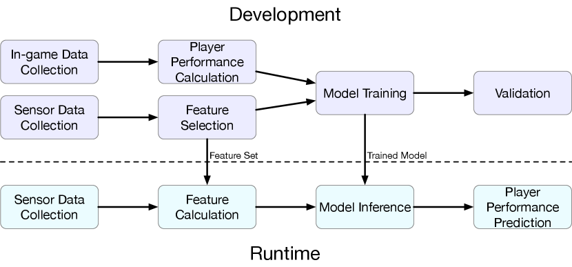
In this section, we describe the sensors used in this research, data collection procedure, data pre-processing, and data analysis helping predict the players performance. In Figure 1 we present an overview of prediction system.
III-A Sensors
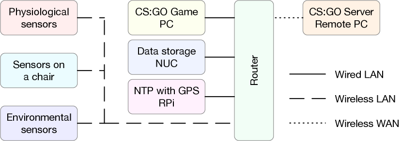
In our work, we use three groups of sensors: physiological sensors, sensors integrated into a game chair, and environmental sensors. The sensor network architecture is shown in Figure 2. The list of sensors used, their locations, and sampling rates are presented in Table I. Further issues associated with sampling rates are discussed in Section III-D1.
| Sensor Group | Sensor | Location | Sampling Rate |
| Physiological Sensors | Electromyography sensor [46] | Elbow | 70 Hz |
| GSR sensor [47] | Fingers | 70 Hz | |
| Heart rate monitor [48] | Chest | 3 Hz | |
| Eye tracker | Under the PC monitor | 90 Hz | |
| Mouse | Hand | 250 Hz | |
| Sensors on a Chair | 3-axis accelerometer and 3-axis gyroscope [49] | The bottom of the chair | 100 Hz |
| Environmental Sensors | CO2 sensor [50] | Environment, 1m from the player | 0.2 Hz |
| Temperature sensor [51] | 5 Hz | ||
| Humidity sensor [52] | 5 Hz |
Physiological data recorded:
-
•
Electromyography (EMG) data as an indicator of muscle activity. EMG data are related to physiological tension affecting player’s current state [53].
-
•
Heart rate data received by a heart rate monitor on a chest. High values correspond to mental stress and arousal [54], which might affect the rationality of player decisions.
-
•
Electrodermal activity (GSR) or skin resistance data as a measure of person arousal [55]. This value is also connected with the stress level.
-
•
Eye tracker data of player gaze position on a monitor in pixel values. The player must check the minimap and other indicators on the screen to have relevant information about the game and, thus, make effective decisions [8].
-
•
Mouse movements captured by a custom python script as a measure of the intensity of a player input. This data is an indirect indicator of the hand movement activity as well as the player skill [9].
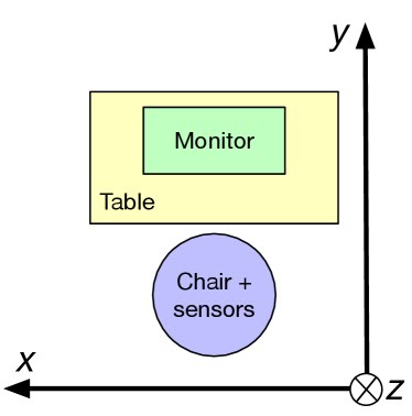
The sensors integrated into a game chair are presented by a 3-axial accelerometer and a 3-axial gyroscope. We illustrate axes orientation for the chair in Figure 3. Recorded data includes:
- •
-
•
Angular velocity of a chair. This data provides the information about the person’s wiggling and spinnings on a chair.
Environmental data recorded:
-
•
level. High level results in the reduction of cognitive abilities [56], thus directly affect the gaming process.
-
•
Relative humidity. High level of relative humidity results in the reduction of neurobehavioral performance [57]
-
•
Environmental temperature. Too warm conditions may affect the human performance [58].
III-B Sensor Network and Synchronization
Apart from a number of heterogeneous sensors, the sensor network has a dedicated storage server (based on Intel NUC PC), gamer PC (a high-speed Intel I7 PC with the DDR4 memory, and an advanced GPU card). For synchronization reasons, we have an NTP server with GPS/PPS support. A high-speed wireless router connects all the devices in the network. PC with strict requirements to ping value (gamer PC, NTP server) has a wired connection to the router (LAN). The sensors have a wireless connection to the network as they are placed near the eSports athletes (WLAN). The router has a low latency connection to the Internet (WAN). Proper synchronization of the sensors and gamer PC is essential for further data collection and analysis.
III-B1 NTP Server
At present, there are many options for building time-synchronous systems for industrial applications, e.g., TSN by NI111http://www.ni.com/white-paper/54730/en/. At the same time, there must be a reasonable balance between the cost of synchronization solution and its accuracy. The cost of most industrial solutions is high, preventing them from integrating into the player’s PC. It happens since the desktop computers are primarily selected according to the 3D games performance criteria and do not have specific hardware devices on board. That is why we decided to realize the synchronization on a single NTP server. A reliable and always available server which could be located close enough and characterized by the minimum delay in transmitting the packets over the network is vital for our sensor network.
A single-board computer Raspberry PI 3B was selected as a server, and a GPS signal was used as a source of reasonably accurate time. The signal from the satellite was received by a separate module based on the MTK MT3333 chipset and having the UART interface as well as supporting the PPS signal on Raspbian Stretch OS, GPS support packages (gpsd, gpsd -clients, pps-tools) and Chrony time server was installed. Raspberry PI was located near the window for better satellite signal reception and connected to the local area network via a wired interface. The presence of a dedicated PPS signal acquired by a separate IO pin (GPIO) Raspberry PI made it possible to ensure time accuracy in the range of s (time accuracy of us).
III-B2 Sensors
The sensors in our network are deployed on Raspberry PI (RPi). The broadcast network ”sync” command was sent to the sensors prior to measurements. After the command reception, a custom made script synchronized the local time to the local NTP server (Stratum 1) time on each RPI. Feedback status with the current time difference was also reported from every RPI to the local data storage PC. In this case, all RPI were synchronized before the measurement procedure starts. Time drift of local RPI time was measured: it is in the range per hour. In this case, the sync command was repeated every minutes. This allows us to have synchronized sensors all the time.
III-B3 Gamer PC Synchronization
Performing the time synchronization on a gamer PC was another significant issue. The players used MS Windows OS on their PCs which do not provide the accurate time to the user by default (you can check how accurate the clock on your PC is at www.time.is). The default settings in Windows 7/8/10 allow the users to synchronize time with the NTP server only once a week. At the same time, the average time drift of the clock is 50 per hour and even more for an ordinary PC according to our measurements. In MS Windows 10 OS build 1607 and newer, there is a way to reduce the synchronization period and get significantly higher time accuracy by setting the registry.
Then Windows Time Service should be switched to Auto (always loaded after the PC starts) start mode.
The accuracy of the clock within 1 requires to meet a number of conditions222https://docs.microsoft.com/en-us/windows-server/networking/windows-time-service/support-boundary. In our experiment (taking into account the local time server Stratum 1 based on RPI), all the requirements were met with the exception of the ping value (it was ms, instead of the required value ms). However, it allows us to achieve the necessary synchronization accuracy.
In the case of proper registry settings after some time, the drift is compensated by the internal Windows algorithms, and the clocks become synchronous with the time server (within accuracy).
Upon synchronizing the hardware in the network, we start the data collection procedure.
III-C Data Collection
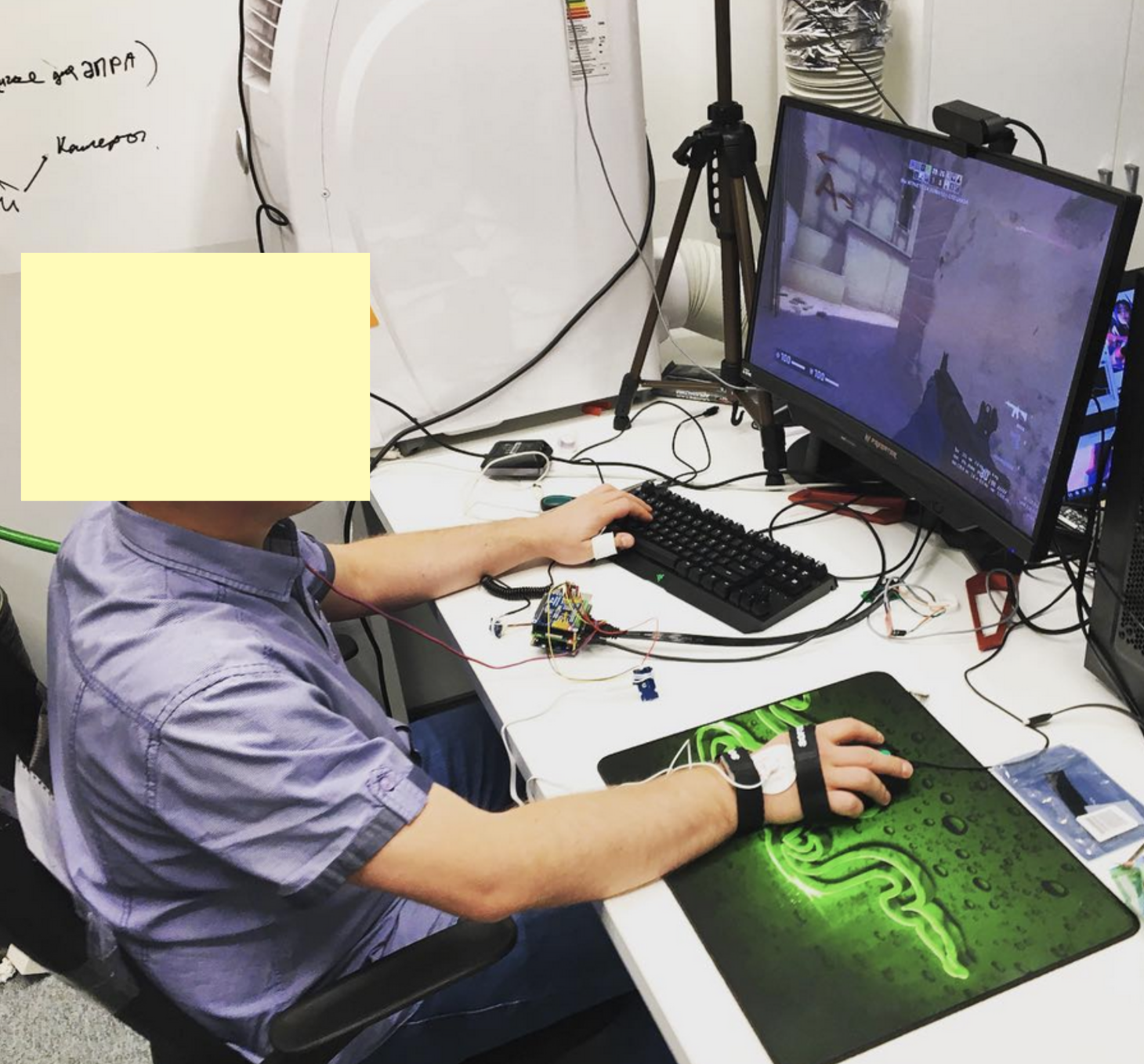
We invited 21 participants to play FPS Counter-Strike: Global Offensive (CS:GO) for 30-35 minutes. We note here that six pro-players took part in this experiment. All the participants were informed about the project and the experimental details. Every participant signed a written consent form which allowed recording physiological and in-game data. Then players were equipped with the sensors for data collection. We did not receive any complaints about the uncomfortable gaming experience because of the sensors. The experimental testbed is snown in Figure 4.
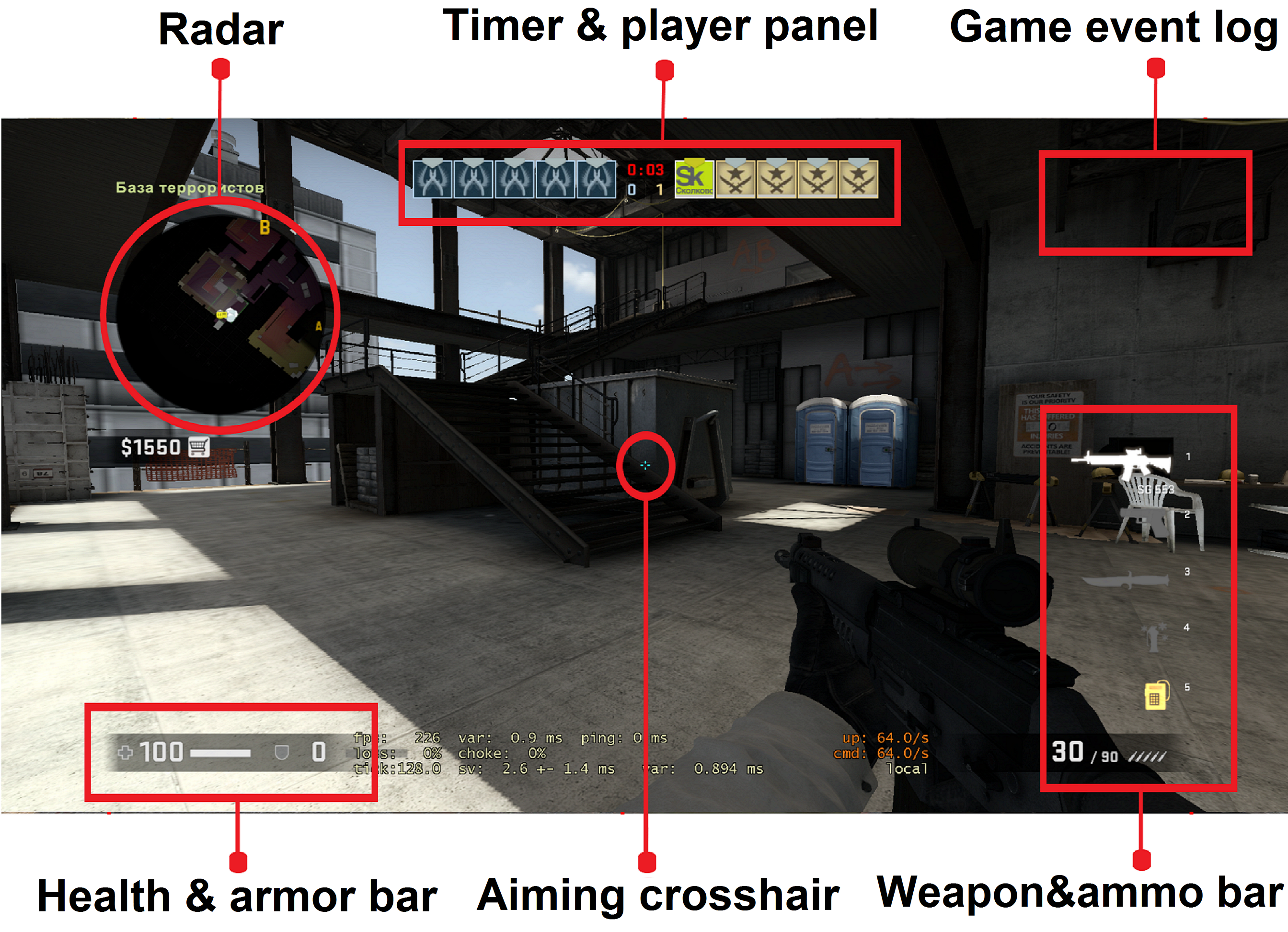
Players needed to play Deathmatch mode of CS:GO. The example of the game screen interface is shown in Figure 5. In this mode the goal of each player is to achieve as many kills of other players as possible and to minimize the number of their own deaths. When the player is killed it immediately respawns in a random location in the game. This mode is often used by eSports players in their training routine. After the game had been finished, we saved the replays for the future game events extraction.
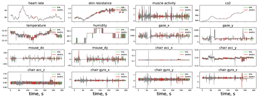
Collected data samples for the 5-minutes intervals for two players are shown in Figure 6. For the reader convenience, we color the intervals in the 1-second vicinity of kill and death events.
It is clear that for the data from some physiological indicators, e.g. skin resistance or heart rate, there are global and local trends, which might align with changes in the player’s efficiency in the game. Another point is that the players usually do not move a lot on a gaming chair. However, they can change their posture from time to time, and this event is captured by the IMU on the chair and also might be connected with the game events and player performance.
III-D Data Pre-processing
To get rid of the noise and occasional outliers, we have clipped all the data by 0.5 and 99.5 percentiles and smoothed the data by 100 moving window. We have also reparametrized gaze, mouse, and muscle activity signals. Mouse signal has been converted from and increments to Euclidian distance passed to reflect the mouse speed; gaze data has been transformed from and coordinates to Euclidian distance passed; muscle activity signal has been changed to L1-distance to the reference level for the player in order to represent the intensity of muscle tension. For 3.7% data missed we have used linear interpolation to fill in the unknown values since it provides a stable and accurate approximation.
III-D1 Sensor Data Resampling
In order to predict the player performance at each moment of time, it is convenient to resample the data from all the sensors to the common sampling rate. This helps apply the proposed data analysis for discrete time series predictions, such as hidden Markov models [41] or recurrent neural networks [59].
However, data from different sensors has different underlying nature and should be resampled accordingly. While it is reasonable to average the data within a time step interval for heart rate, skin resistance, muscle activity, environmental data, chair acceleration and rotation, averaging is not applicable for the gaze movement and mouse movement data. The reason behind it is that we are interested in the total distance passed within the time step instead of the average distance passed per measurement. The total distance does not depend on a number of samples, but only on their sum.
Resampling introduces an important hyperparameter time step. Throughout the manuscript we refer to it is as . Big time step values, e.g. 5 minutes, are not meaningful for our problem since we need to extract the relevant information about the player. On the other hand, too small timestamp, e.g 0.1 , may lead to an excessive number of observations and noisier data. Indeed, the resampling time step should not be smaller than the time between the measurements for the majority of sensors.
After converting the sampling rates to the common value we obtained a 15-dimensional feature vector for each moment of time. Further in the paper we will refer to this feature vector as . Its components are described in Table II.
| Feature Group | Feature Name |
|---|---|
| Physiological Activity | Heart Rate |
| Muscle Activity | |
| Skin Resistance | |
| Gaze Movement | |
| Mouse Movement | |
| Mouse Scroll | |
| Chair Movement | Linear Accelerations along axes |
| Angular velocity along axes | |
| Environment | CO2 level |
| Temperature | |
| Humidity |
III-E Player Performance Evaluation
There is no generic player effectiveness metric for the majority of eSports disciplines. The most popular evaluation metric for FPS and MOBA games is Kill Death Ratio (KDR) [60]. It equals the number of kills divided by the number of deaths for the time interval. If KDR ¿ 1, it means that the player performs well, or, at least, better than some players on a game server. Otherwise, the player most likely performs bad compared to other players.
KDR takes values from to which is not a clear range for prediction. When the player performs very well and has many kills and few deaths, KDR is fluctuating drastically because of division by a small number. In opposite, if there are many deaths and few kills, KDR is around 0 and changes slowly. This drastic inconsistency in the target creates difficulties for training machine learning algorithms. One possible solution could be to apply logarithm to KDR, but this does not solve the issue with the scale, because logarithm takes the values from to .
We propose a more numerically stable target value which equals the proportion of kills for the player. More precisely,
| (1) | |||
| (2) | |||
| (3) |
where is the proportion or performance and equals the proportion of kills for a player at the moment considering the kills and death in the next seconds. In other words, it is the ratio of kills in the next seconds. and are the total number of kills and deaths at the moment ; therefore and equals the number of kills and deaths within the interval . varies from 0 to 1 and has higher values for well-performing players. Bounding by 0 and 1 helps efficiently train the machine learning algorithms that are sensitive to the target scale.
The important hyperparameter introduced above is . Essentially, it is a window size for which the information about the future player performance is aggregated. Small values of the hyperparameter like 1 lead to noisy target values, while large values like 10 minutes neglect the subtle yet important changes in the player performance. is commonly referred to as a forecasting horizon.
is a well defined metric for evaluating the player effectiveness, and it is possible to predict this value directly, thus considering the problem as a regression problem. However, it is unclear how to interpret the quality of regression results in an understandable and interpretable way. Formulating the problem in classification terms helps measuring the quality of prediction by more comprehensive classification metrics like accuracy, ROC AUC, and others. These metrics are much easier to compare with results obtained on other data or by other models.
The natural way to claim if a person plays well or bad at the moment is to compare the current performance with his or her average performance in the past. It is important to consider the past events only to avoid overfitting. Formally:
| (4) | |||
| (5) |
where and equals 1 in case of good game performance and 0 otherwise; is an average player performance in the past.
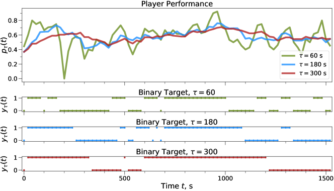
Figure 7 demonstrates how the kills ratio and corresponding binary target changes over time for three forecasting horizons.
The substantial advantage of using instead of is target unification between the players. and values of have the same meaning for all players and imply bad and good current performance, respectively. That is not the case for raw values of , because the same values of may be good for one player, but bad for another one. For example, 0.5 kills ratio may be an achievement for a newbie player, but a failure for a professional player.
Another justification of using as a target is robustness to the skill of other players on a server. Player’s score may be too low in absolute value because of the strong opponents, but target is robust because it evaluates the performance within one game. The motivation for this target is to unify the target variable for all players and to provide in advance an immediate feedback for a player or for a manager that something is going wrong.
Predicting future player performance is essential for coaches and progressing players as it provides the quick feedback on players’ actions. That might help identify the inevitable failures in player performance, e.g. burnout, fatigue, etc., in advance and take measures to help the player to recover or even to change the player during the eSports competition. This target is also helpful for learning purposes: although a person plays very well or very poor, it helps find the moments when the player performs a bit better or worse than average.
Despite we formulate the performance metric in terms of kills/deaths, the metric is directly applicable to the majority of First-Player Shooters, as well as other games including kills/deaths. The performance metrics for these and other games can be calculated in other terms (such as gold, scores, progress, etc.), while the data processing and algorithms may be the same.
III-F Predictive models
We trained four models for predicting a player performance using the data from sensors: baseline model, logistic regression, recurrent neural network, and recurrent neural network with attention. In this section, we describe these methods in detail. The output for all models is the probability that the person will play better in some fixed period in the future. All the models are evaluated by ROC AUC score discussed in section III-G2.
III-F1 Baseline
Before training a complex model, it is crucial to set up a simple baseline to compare it with. A common practice in time series analysis is to establish a baseline model using a current target value as a future prediction. For our problem, the baseline uses average player performance in the last seconds as a prediction. In other words, baseline prediction is . This prediction is correct because takes values from to , and then they treated as probabilities by the algorithm used to calculate the ROC AUC metric.
III-F2 Logistic Regression
Logistic regression [61] is a simple and robust linear classification algorithm. It takes a feature vector as an input at the moment of time and provides the probability equals as an output:
| (6) |
where is the learnable weights vector, is the bias term. In our study, the dimensionality is since we used 15 values from sensors. Logistic regression can capture only linear dependencies in the data because the feature vector involved in dot product with vector only.
III-F3 Recurrent Neural Network
A neural network can be considered as a nonlinear generalization of logistic regression. In this subsection, we first describe the essential components used in the network and then describe the entire architecture.
Recurrent Neural Network Background
A Recurrent Neural Network (RNN) is a network that maintains an internal state inherent to some sequence of events. It is proven to be efficient for discrete time series prediction [59]. One of the simplest examples of RNN is a neural network with one hidden layer.
Denote the sequence of input features and targets as and respectively, where is the -dimensional feature vector for the moment , is the corresponding target, is the time step used for discretization, is the total number of steps.
At each moment , the recurrent network has an -dimensional hidden state vector which is calculated using the current input and the previous hidden state :
| (7) |
where , , are the learnable matrices and the bias vector.
The intuition behind using the RNN architecture might be in considering the hidden state of the network as a current state of the player represented by the data from sensors. The state is a vector with many components and some of them can present how well the person will play. The final prediction at the moment is calculated by the feed-forward network consisting of or more linear layers:
| (8) |
where is the function corresponding to the feed-forward network. We used a sigmoid function as a final activation for the network to ensure , so has a meaning of probability.
Gated Recurrent Unit
More advanced modifications of the recurrent layer include the Gated Recurrent Unit (GRU) [62] and Long Short-Term Memory (LSTM) [63]. Both of them utilize the gating mechanism to better control the flow of information. LSTM architecture incorporates an input, output, and forget gates and a memory cell, while a simpler GRU architecture uses the update and reset gates only. We found GRU performs better in our task, so we formally define it as follows:
| (9) | |||
| (10) | |||
| (11) | |||
| (12) |
where and are the update and reset gates, are the learnable parameters, is Hadamard product, is the sigmoid function.
Attention Mechanism
A popular technique for improving the network quality and interpretability is an attention mechanism. Temporal attention can help emphasize the relevant hidden states from the past. Input attention helps to select the essential input features. It is also possible to combine both of them [64]. Since the proposed GRU model uses only one previous hidden state for prediction, it makes no sense to use the temporal attention. However, the input attention can be used.
The attention layer provides the weights vector , which is applied to a vector by the element-wise multiplication:
| (13) |
This operation demonstrates important components in the vector while decreasing the contribution of its non-relevant components. Typically, components are bounded by and and produced by another linear layer integrated into the network. In order to consider both the current and the previous data from sensors, the attention layer takes current measurements and hidden state produced by GRU:
| (14) |
where the are trainable parameters.
The intuition behind the input attention mechanism is a feature selection. Based on the current input and hidden state, it can help ignoring the uninformative features for each moment of time and keep relevant features unaltered. The ability to provide the time-dependent feature importance is a significant advantage compared to other methods, which can either provide feature importance for one particular moment or provide it only for the whole time series.
Recurrent Neural Network With Attention Architecture
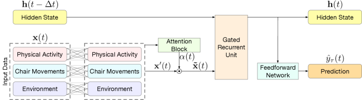
The neural network architecture is shown in Figure 8. First, the sensor data are processed by the dense layers for each feature group. Then the attention block is applied to amplify a signal from the features relevant at the moment. The resulting vector goes through the GRU cell to update the hidden state . This hidden state is saved for further iterations and goes through a feed-forward network to form the eventual prediction . The total inference time is about 5 on a CPU.
The network was trained by the truncated backpropagation through time [65] technique designed for RNNs and Adam optimizer [66] with learning rate warmup [67] technique to improve the convergence. For attention and feed-forward networks, we used and linear layers, respectively, with ReLU nonlinearity. This activation function can improve the convergence and numerical stability [68]. To validate whether the attention mechanism helps improve network performance, we also trained another network without the attention block.
GRU cell is a crucial part of the network architecture. It helps accumulate information about previous player states, so the network can use the retrospective context for prediction. This information is stored in the hidden layer of the GRU cell. According to the experiments, 8 neurons in the hidden layer works for our problem the best. Too few neurons caused low predictive power, while too many led to overfitting.
The motivation to use separate linear layers for three feature groups is to combine more complex features from the sensors data and to preserve the disentangled feature representation for the attention layer. This is an analog of grouped convolutions [69] in convolutional networks. For the same reasons, we applied the attention to each feature group separately, thus having a 3-dimensional attention vector at each moment of time.
III-G Validation
III-G1 Training and Evaluation Process
In order to correctly estimate the generalization capabilities of classical machine learning algorithms, we used repeated cross-validation [70]. In particular, we randomly split 21 players into the train and test groups of 16 and 5 players, respectively. Then we trained the algorithms and repeated this procedure again 100 times. It helps to lower the variance in evaluation.
For neural networks, we also used a validation set, so we randomly split players into train, validation, and test sets with 11, 5, and 5 players, respectively. The neural network has been trained until the error on the validation set is not improving for 5 epochs (early stopping procedure). One training epoch comprises of 20 batches. Each batch consists of input features and targets for all the time steps for a randomly selected player from the train set. To minimize the randomness in the evaluation results, each network has been trained 15 times with random weight initializations and train/val/test split. In both cases, the input features for train, test, and validation sets are normalized based on the mean values and standard deviations calculated on the train set.
III-G2 Evaluation Metric
Due to construction, the target is balanced: 50.1% belong to the positive class and 49.9% to the negative class. The common metric for classification evaluation is the area under the receiver operating characteristic curve (ROC AUC) [71]. It ranges from to with the score for random guessing. Higher values are better.
For proper evaluation, we first calculated the ROC AUC scores for each individual participant in the train, validation, or test sets, and then averaged the results. That is the proper evaluation because it estimates how well the model can separate the high/low performance conditions for one individual participant and does not benefit from separating the participants between themselves in the case when the metric is calculated on predictions for all the participants.
IV Results
IV-A Performance of Algorithms
We have trained the predictive models for several time steps (see Section III-D1) and forecasting horizons (see Section III-E) combinations. According to our experiments, reasonable ranges are from 5 to 30 for time step, and from 60 to 300 for the forecasting horizon. The average results for the neural network with attention are shown in Table III.
| Forecasting Horizon , s | Time Step , s | |||||
|---|---|---|---|---|---|---|
| 5 | 10 | 15 | 20 | 24 | 30 | |
| 60 | 0.602 | 0.658 | 0.632 | 0.617 | 0.645 | 0.689 |
| 120 | 0.609 | 0.621 | 0.682 | 0.631 | 0.680 | 0.657 |
| 180 | 0.611 | 0.622 | 0.652 | 0.711 | 0.682 | 0.642 |
| 240 | 0.667 | 0.661 | 0.654 | 0.726 | 0.724 | 0.703 |
| 300 | 0.619 | 0.667 | 0.721 | 0.680 | 0.717 | 0.724 |
According to Table III, the best time step value is about 20 , and the best forecasting horizon for the model is from 3 to 5 minutes. In other words, the optimal way to predict the player behavior is to aggregate the sensors data every 20 and make a prediction for the next 3-5 minutes.
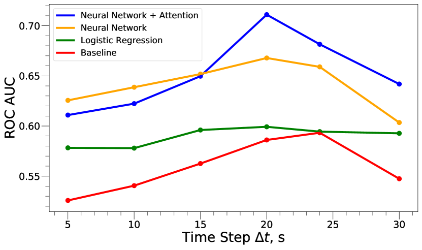
We have compared the performance of the algorithms described in Section III-F with respect to the time step values with fixed forecasting horizon equal 180 . The results are shown in Figure 9. There is a clear peak near 20-25 for all the methods. The neural network consistently outperforms the logistic regression and the baseline model. The use of the attention block helps increase the model score.
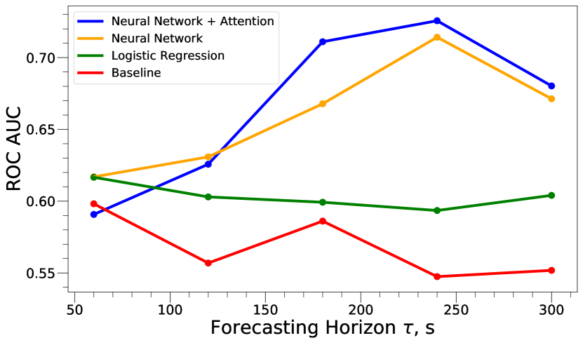
Figure 10 demonstrates the relation between the forecasting horizon and algorithms performance with the time step equal to 20 . The neural network outperforms other methods and achieves the maximum performance for forecasting horizons in the range from 3 to 5 minutes. The attention block helps improve the model.
IV-B Feature importance
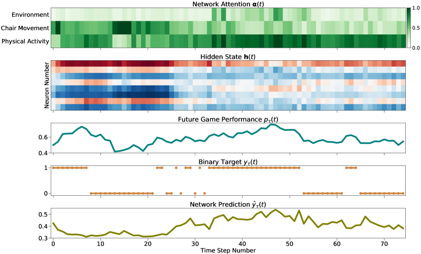
In order to interpret the neural network predictions, we calculated the feature importances and visualized predictions of a pretrained network and its internal state for the discretization step equal to 20 and the forecasting horizon equal to 3 minutes. Figure 11 shows how attention, network hidden state, target, and network prediction change over time. Clearly, the importance of different features varies over time, and periodically the data from some sensors is non-relevant. The network hidden state, which can be treated as a player state, also varies during the game.
To calculate the feature importance, we trained 100 instances of the neural network with random weight initializations and the train/val/test splits, and the averaged attentions on the test set for the best epoch of each neural network. Afterwards, we averaged the results across all networks. The results are shown in Table IV and Figure 12.
| Feature Group | Mean Attention |
|---|---|
| Physiological Activity | 0.228 |
| Chair Movement | 0.207 |
| Environment | 0.197 |
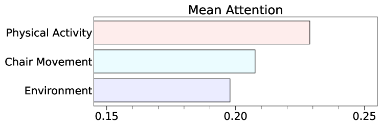
Information about physiological activity such as heart rate, muscle activity, hand movement, and so on is the most relevant for the network. It is worth noting that all the feature groups have considerable importance, thus contribute to the overall prediction. Since the features in each feature group are mixed, we can not estimate the feature importance for every raw feature.
IV-C Discussion
Experimental results have shown practical feasibility of predicting the eSports players behavior using only data from sensors. The system updates the prediction several times per minute, so this interactivity is enough for potential users like eSports managers or professional players to understand that something goes wrong or to get a quick feedback. Feedback from the algorithm about the performance prediction and feature importance may suggest the users to change their gaming behavior. For example, an eSports manager may understand in time that bad results of the team are connected with the stuffy environmental conditions and adjust the air conditioning. Users may find information from the system useful to make the radical decisions, e.g., changing a player or gaming equipment (computer mouse, display, game chair, etc.).
We have found that 20 time step and 3-5 minutes behavior forecasting horizon are the most natural parameters for CS:GO, but potential users can set up any other hyperparameters depending on their scenario. Significant advantage caused by the diversified training dataset is universality for the player skill level enabling a wide range of potential users. Negligible model inference time and data collection time on a PC proves the principal feasibility of deploying the model on the edge devices, some of which might be designed specifically for neural network operations. However, the model retraining still requires high computational capability. Larger and more diversified dataset could improve the performance of prediction.
IV-D Limitations
The limitations of the study is a small number of participants involved, the fuzziness of the definition of player’s performance, and overrepresentation of data from males and young people in the dataset. Future work includes more diverse and extensive data collection with more subjects recorded, and the investigation of better metrics of players’ performance. These would allow researchers to utilize more complex machine learning methods and to develop more reliable and robust models.
V Conclusions
In this article, we have reported on the AI-enabled system for predicting the performance of eSports players using only the data from heterogeneous sensors. The system consists of a number of sensors capable of recording players’ physiological data, movements on the game chair, and environmental conditions. Upon data collection we have processed them into time series with meaningful sensors features and the target extracted from the game events. The Recurrent Neural Network (RNN) demonstrated the best performance comparing to baseline and logistic regression. Application of the attention mechanism for RNN has helped to interpret the network predictions as well as to extract the feature importances. Our work showed the connection between the player performance and the data from sensors as well as the possibility of making a real-time system for training and forecasting in eSports.
We have also investigated potential applications of the proposed AI system in the eSports domain. Given the growth of eSports activity due to the coronavirus pandemic in 2019–2021 and rapid development of consumer wearable devices within the last years, this work shows the prospectives of full-fledged research in the intersection of these two fields. Moreover, the model trained on the eSports domain can be transferred to other domains using domain adaptation methods to estimate user’s performance similar to estimating in-game performance.
Considering hunders of millions of active gamers in the world and widespread of wearables, crowdsourcing data collection is a promising way to collect the data on a global scale. We also see potential improvements in our system with computer vision methods. Emotion recognition and pose estimation techniques applied to data collected from web camera can provide more information about the current state of a player.
Acknowledgment
The reported study was funded by RFBR according to the research project No. 18-29-22077.
Authors would like to thank professional eSports team DreamEaters for fruitful discussions and data collection.
References
- [1] C. G. Anderson, A. M. Tsaasan, J. Reitman, J. S. Lee, M. Wu, H. Steel, T. Turner, and C. Steinkuehler, “Understanding esports as a stem career ready curriculum in the wild,” in 2018 10th International Conference on Virtual Worlds and Games for Serious Applications (VS-Games), Sept 2018, pp. 1–6.
- [2] Newzoo. (2018) Global esports market report. [Online]. Available: https://asociacionempresarialesports.es/wp-content/uploads/newzoo_2018_global_esports_market_report_excerpt.pdf
- [3] D. J. Diaz-Romero, A. M. R. Rincón, A. Miguel-Cruz, N. Yee, and E. Stroulia, “Recognizing emotional states with wearables while playing a serious game,” IEEE Transactions on Instrumentation and Measurement, vol. 70, pp. 1–12, 2021.
- [4] M. Z. Baig and M. Kavakli, “A survey on psycho-physiological analysis & measurement methods in multimodal systems,” Multimodal Technologies and Interaction, vol. 3, no. 2, p. 37, 2019.
- [5] T. Tuncer, F. Ertam, S. Dogan, and A. Subasi, “An automated daily sports activities and gender recognition method based on novel multikernel local diamond pattern using sensor signals,” IEEE Transactions on Instrumentation and Measurement, vol. 69, no. 12, pp. 9441–9448, 2020.
- [6] A. Drachen, L. E. Nacke, G. Yannakakis, and A. L. Pedersen, “Correlation between heart rate, electrodermal activity and player experience in first-person shooter games,” in Proceedings of the 5th ACM SIGGRAPH Symposium on Video Games. ACM, 2010, pp. 49–54.
- [7] P. Mavromoustakos Blom, S. Bakkes, and P. Spronck, “Towards multi-modal stress response modelling in competitive league of legends,” 08 2019, pp. 1–4.
- [8] B. B. Velichkovsky, N. Khromov, A. Korotin, E. Burnaev, and A. Somov, “Visual fixations duration as an indicator of skill level in esports,” in Human-Computer Interaction – INTERACT 2019, D. Lamas, F. Loizides, L. Nacke, H. Petrie, M. Winckler, and P. Zaphiris, Eds. Cham: Springer International Publishing, 2019, pp. 397–405.
- [9] D. Buckley, K. Chen, and J. Knowles, “Predicting skill from gameplay input to a first-person shooter,” in 2013 IEEE Conference on Computational Inteligence in Games (CIG). IEEE, 2013, pp. 1–8.
- [10] N. Khromov, A. Korotin, A. Lange, A. Stepanov, E. Burnaev, and A. Somov, “Esports athletes and players: a comparative study,” arXiv preprint arXiv:1812.03200, 2018.
- [11] A. Smerdov, A. Kiskun, R. Shaniiazov, A. Somov, and E. Burnaev, “Understanding cyber athletes behaviour through a smart chair: Cs:go and monolith team scenario,” in 2019 IEEE 5th World Forum on Internet of Things (WF-IoT), April 2019, pp. 973–978.
- [12] A. Smerdov, E. Burnaev, and A. Somov, “esports pro-players behavior during the game events: Statistical analysis of data obtained using the smart chair,” in 2019 IEEE SmartWorld, Ubiquitous Intelligence Computing, Advanced Trusted Computing, Scalable Computing Communications, Cloud Big Data Computing, Internet of People and Smart City Innovation (SmartWorld/SCALCOM/UIC/ATC/CBDCom/IOP/SCI), 2019, pp. 1768–1775.
- [13] J. Haladjian, D. Schlabbers, S. Taheri, M. Tharr, and B. Bruegge, “Sensor-based detection and classification of soccer goalkeeper training exercises,” ACM Transactions on Internet of Things, vol. 1, no. 2, pp. 1–20, 2020.
- [14] T. Stone, N. Stone, N. Roy, W. Melton, J. B. Jackson, and S. Nelakuditi, “On smart soccer ball as a head impact sensor,” IEEE Transactions on Instrumentation and Measurement, vol. 68, no. 8, pp. 2979–2987, 2019.
- [15] B. Groh, M. Fleckenstein, T. Kautz, and B. Eskofier, “Classification and visualization of skateboard tricks using wearable sensors,” Pervasive and Mobile Computing, vol. 40, pp. 42 – 55, 2017. [Online]. Available: http://www.sciencedirect.com/science/article/pii/S1574119217302833
- [16] J. Wang, Z. Wang, F. Gao, H. Zhao, S. Qiu, and J. Li, “Swimming stroke phase segmentation based on wearable motion capture technique,” IEEE Transactions on Instrumentation and Measurement, vol. 69, no. 10, pp. 8526–8538, 2020.
- [17] Z. Wang, J. Li, J. Wang, H. Zhao, S. Qiu, N. Yang, and X. Shi, “Inertial sensor-based analysis of equestrian sports between beginner and professional riders under different horse gaits,” IEEE Transactions on Instrumentation and Measurement, vol. 67, no. 11, pp. 2692–2704, 2018.
- [18] B. Andò, V. Marletta, S. Baglio, R. Crispino, G. Mostile, V. Dibilio, A. Nicoletti, and M. Zappia, “A measurement system to monitor postural behavior: Strategy assessment and classification rating,” IEEE Transactions on Instrumentation and Measurement, vol. 69, no. 10, pp. 8020–8031, 2020.
- [19] V. Hodge, S. Devlin, N. Sephton, F. Block, A. Drachen, and P. Cowling, “Win prediction in esports: Mixed-rank match prediction in multi-player online battle arena games,” arXiv preprint arXiv:1711.06498, 2017.
- [20] L. Lin, “League of legends match outcome prediction.”
- [21] T. D. Smithies, M. J. Campbell, N. Ramsbottom, and A. J. Toth, “A random forest approach to identify metrics that best predict match outcome and player ranking in the esport rocket league,” 2021.
- [22] Y. Yang, T. Qin, and Y.-H. Lei, “Real-time esports match result prediction,” arXiv preprint arXiv:1701.03162, 2016.
- [23] I. Makarov, D. Savostyanov, B. Litvyakov, and D. I. Ignatov, “Predicting winning team and probabilistic ratings in “dota 2” and “counter-strike: Global offensive” video games,” in International Conference on Analysis of Images, Social Networks and Texts. Springer, 2017, pp. 183–196.
- [24] A. Drachen, R. Sifa, C. Bauckhage, and C. Thurau, “Guns, swords and data: Clustering of player behavior in computer games in the wild (pre-print),” 09 2012.
- [25] L. Gao, J. Judd, D. Wong, and J. Lowder, “Classifying dota 2 hero characters based on play style and performance,” Univ. of Utah Course on ML, 2013.
- [26] C. Eggert, M. Herrlich, J. Smeddinck, and R. Malaka, “Classification of player roles in the team-based multi-player game dota 2,” in International Conference on Entertainment Computing. Springer, 2015, pp. 112–125.
- [27] M. Märtens, S. Shen, A. Iosup, and F. Kuipers, “Toxicity detection in multiplayer online games,” in 2015 International Workshop on Network and Systems Support for Games (NetGames). IEEE, 2015, pp. 1–6.
- [28] M. Viggiato and C.-P. Bezemer, “Trouncing in dota 2: An investigation of blowout matches,” in Proceedings of the AAAI Conference on Artificial Intelligence and Interactive Digital Entertainment, vol. 16, no. 1, 2020, pp. 294–300.
- [29] D. J. Cornforth and M. T. Adam, “Cluster evaluation, description, and interpretation for serious games,” in Serious Games Analytics. Springer, 2015, pp. 135–155.
- [30] S. Saponara, “Wearable biometric performance measurement system for combat sports,” IEEE Transactions on Instrumentation and Measurement, vol. 66, no. 10, pp. 2545–2555, 2017.
- [31] Y. Wang, Y. Zhao, R. H. Chan, and W. J. Li, “Volleyball skill assessment using a single wearable micro inertial measurement unit at wrist,” IEEE Access, vol. 6, pp. 13 758–13 765, 2018.
- [32] A. Ahmadi, D. Rowlands, and D. A. James, “Towards a wearable device for skill assessment and skill acquisition of a tennis player during the first serve,” Sports Technology, vol. 2, no. 3-4, pp. 129–136, 2009.
- [33] A. Ahmadi, D. D. Rowlands, and D. A. James, “Investigating the translational and rotational motion of the swing using accelerometers for athlete skill assessment,” in SENSORS, 2006 IEEE. IEEE, 2006, pp. 980–983.
- [34] C. Ladha, N. Y. Hammerla, P. Olivier, and T. Plötz, “Climbax: skill assessment for climbing enthusiasts,” in Proceedings of the 2013 ACM international joint conference on Pervasive and ubiquitous computing. ACM, 2013, pp. 235–244.
- [35] O. Yuji, “Mems sensor application for the motion analysis in sports science,” Memory, vol. 32, p. 128Mbit, 2005.
- [36] M. Kranz, A. MöLler, N. Hammerla, S. Diewald, T. PlöTz, P. Olivier, and L. Roalter, “The mobile fitness coach: Towards individualized skill assessment using personalized mobile devices,” Pervasive and Mobile Computing, vol. 9, no. 2, pp. 203–215, 2013.
- [37] S. Matsumura, K. Ohta, S.-i. Yamamoto, Y. Koike, and T. Kimura, “Comfortable and convenient turning skill assessment for alpine skiers using imu and plantar pressure distribution sensors,” Sensors, vol. 21, no. 3, p. 834, 2021.
- [38] A. Khan, S. Mellor, E. Berlin, R. Thompson, R. McNaney, P. Olivier, and T. Plötz, “Beyond activity recognition: skill assessment from accelerometer data,” in Proceedings of the 2015 ACM International Joint Conference on Pervasive and Ubiquitous Computing. ACM, 2015, pp. 1155–1166.
- [39] M. Ershad, R. Rege, and A. M. Fey, “Automatic surgical skill rating using stylistic behavior components,” in 2018 40th Annual International Conference of the IEEE Engineering in Medicine and Biology Society (EMBC). IEEE, 2018, pp. 1829–1832.
- [40] N. Ahmidi, G. D. Hager, L. Ishii, G. Fichtinger, G. L. Gallia, and M. Ishii, “Surgical task and skill classification from eye tracking and tool motion in minimally invasive surgery,” in International Conference on Medical Image Computing and Computer-Assisted Intervention. Springer, 2010, pp. 295–302.
- [41] P. Dymarski, Hidden Markov Models: Theory and Applications. BoD–Books on Demand, 2011.
- [42] H. Yamanaka, K. Makiyama, K. Osaka, M. Nagasaka, M. Ogata, T. Yamada, and Y. Kubota, “Measurement of the physical properties during laparoscopic surgery performed on pigs by using forceps with pressure sensors,” Advances in urology, vol. 2015, 2015.
- [43] K. Kodama, K. Ioi, and Y. Ohtsubo, “Development of a new skill acquisition tool and evaluation of mold-polishing skills,” in Proc. of the 34Th Chinese Control Conference and Sice Annual Conference, 2015, pp. 139–142.
- [44] T. Yamamoto and T. Fujinami, “Hierarchical organization of the coordinative structure of the skill of clay kneading,” Human movement science, vol. 27, no. 5, pp. 812–822, 2008.
- [45] M. Xochicale, C. Baber, and M. Oussalah, “Analysis of the movement variability in dance activities using wearable sensors,” in Wearable Robotics: Challenges and Trends. Springer, 2017, pp. 149–154.
- [46] S. T. Inc., “Grove–emg detector,” Tech. Rep., 2015. [Online]. Available: https://www.mouser.com/datasheet/2/744/Seeed_101020058-1217528.pdf
- [47] ——, “Grove - gsr,” Tech. Rep., 2015. [Online]. Available: https://www.mouser.com/catalog/specsheets/Seeed_101020052.pdf
- [48] G. Ltd., “Heart rate monitor,” Tech. Rep., 2012. [Online]. Available: http://static.garmin.com/pumac/HRM_Soft_Strap_ML_Web.pdf
- [49] I. Inc., “Mpu-9250 product specification,” Tech. Rep., 2016. [Online]. Available: https://invensense.tdk.com/wp-content/uploads/2015/02/PS-MPU-9250A-01-v1.1.pdf
- [50] L. Zhengzhou Winsen Electronics Technology Co., “Intelligent infrared co2 module,” Tech. Rep., 2016. [Online]. Available: https://www.winsen-sensor.com/d/files/infrared-gas-sensor/mh-z19b-co2-ver1_0.pdf
- [51] I. Digilent, “Pmodtmp3 reference manual,” Tech. Rep., 2016. [Online]. Available: https://reference.digilentinc.com/_media/reference/pmod/pmodtmp3/pmodtmp3_rm.pdf
- [52] ——, “Pmod hygro reference manual,” Tech. Rep., 2017. [Online]. Available: https://reference.digilentinc.com/_media/reference/pmod/pmodhygro/pmod-hygro-rm.pdf
- [53] P. M. Lehrer, D. M. Batey, R. L. Woolfolk, A. Remde, and T. Garlick, “The effect of repeated tense-release sequences on emg and self-report of muscle tension: An evaluation of jacobsonian and post-jacobsonian assumptions about progressive relaxation,” Psychophysiology, vol. 25, no. 5, pp. 562–569, 1988.
- [54] J. Taelman, S. Vandeput, A. Spaepen, and S. Van Huffel, “Influence of mental stress on heart rate and heart rate variability,” in 4th European conference of the international federation for medical and biological engineering. Springer, 2009, pp. 1366–1369.
- [55] D. C. Fowles, “The three arousal model: Implications of gray’s two-factor learning theory for heart rate, electrodermal activity, and psychopathy,” Psychophysiology, vol. 17, no. 2, pp. 87–104, 1980.
- [56] J. G. Allen, P. MacNaughton, U. Satish, S. Santanam, J. Vallarino, and J. D. Spengler, “Associations of cognitive function scores with carbon dioxide, ventilation, and volatile organic compound exposures in office workers: a controlled exposure study of green and conventional office environments,” Environmental health perspectives, vol. 124, no. 6, pp. 805–812, 2016.
- [57] M. Zhu, W. Liu, and P. Wargocki, “Changes in eeg signals during the cognitive activity at varying air temperature and relative humidity,” Journal of Exposure Science & Environmental Epidemiology, vol. 30, no. 2, pp. 285–298, 2020.
- [58] L. Lan, P. Wargocki, D. P. Wyon, and Z. Lian, “Effects of thermal discomfort in an office on perceived air quality, sbs symptoms, physiological responses, and human performance,” Indoor air, vol. 21, no. 5, pp. 376–390, 2011.
- [59] A. C. Tsoi and A. Back, “Discrete time recurrent neural network architectures: A unifying review,” Neurocomputing, vol. 15, no. 3-4, pp. 183–223, 1997.
- [60] K. J. Shim, K.-W. Hsu, S. Damania, C. DeLong, and J. Srivastava, “An exploratory study of player and team performance in multiplayer first-person-shooter games,” in 2011 IEEE Third International Conference on Privacy, Security, Risk and Trust and 2011 IEEE Third International Conference on Social Computing. IEEE, 2011, pp. 617–620.
- [61] D. G. Kleinbaum, K. Dietz, M. Gail, M. Klein, and M. Klein, Logistic regression. Springer, 2002.
- [62] R. Dey and F. M. Salemt, “Gate-variants of gated recurrent unit (gru) neural networks,” in 2017 IEEE 60th international midwest symposium on circuits and systems (MWSCAS). IEEE, 2017, pp. 1597–1600.
- [63] S. Hochreiter and J. Schmidhuber, “Long short-term memory,” Neural computation, vol. 9, no. 8, pp. 1735–1780, 1997.
- [64] Y. Qin, D. Song, H. Chen, W. Cheng, G. Jiang, and G. Cottrell, “A dual-stage attention-based recurrent neural network for time series prediction,” arXiv preprint arXiv:1704.02971, 2017.
- [65] H. Tang and J. Glass, “On training recurrent networks with truncated backpropagation through time in speech recognition,” in 2018 IEEE Spoken Language Technology Workshop (SLT). IEEE, 2018, pp. 48–55.
- [66] D. P. Kingma and J. Ba, “Adam: A method for stochastic optimization,” arXiv preprint arXiv:1412.6980, 2014.
- [67] L. Liu, H. Jiang, P. He, W. Chen, X. Liu, J. Gao, and J. Han, “On the variance of the adaptive learning rate and beyond,” arXiv preprint arXiv:1908.03265, 2019.
- [68] K. Hara, D. Saito, and H. Shouno, “Analysis of function of rectified linear unit used in deep learning,” in 2015 International Joint Conference on Neural Networks (IJCNN). IEEE, 2015, pp. 1–8.
- [69] S. Yi, J. Ju, M.-K. Yoon, and J. Choi, “Grouped convolutional neural networks for multivariate time series,” arXiv preprint arXiv:1703.09938, 2017.
- [70] J.-H. Kim, “Estimating classification error rate: Repeated cross-validation, repeated hold-out and bootstrap,” Computational statistics & data analysis, vol. 53, no. 11, pp. 3735–3745, 2009.
- [71] J. Fan, S. Upadhye, and A. Worster, “Understanding receiver operating characteristic (roc) curves,” Canadian Journal of Emergency Medicine, vol. 8, no. 1, pp. 19–20, 2006.