Aging Exponents for Nonequilibrium Dynamics following Quenches from Critical Point
Abstract
Via Monte Carlo simulations we study nonequilibrium dynamics in the nearest-neighbor Ising model, following quenches to points inside the ordered region of the phase diagram. With the broad objective of quantifying the nonequilibrium universality classes corresponding to spatially correlated and uncorrelated initial configurations, in this paper we present results for the decay of the order-parameter autocorrelation function for quenches from the critical point. This autocorrelation is an important probe for the aging dynamics in far-from-equilibrium systems and typically exhibits power-law scaling. From the state-of-the-art analysis of the simulation results we quantify the corresponding exponents () for both conserved and nonconserved (order parameter) dynamics of the model, in space dimension . Via structural analysis we demonstrate that the exponents satisfy a bound. We also revisit the case to obtain more accurate results. It appears that irrespective of the dimension, is same for both conserved and nonconserved dynamics.
I Introduction
Following a quench from high temperature disordered phase to a point inside the ordered region, when a homogeneous system evolves towards the new equilibrium, several quantities bray_adv ; binder_cahn ; onuki ; ral ; bray_majumdar ; zannetti ; fisher_huse are of importance for the understanding of the nonequilibrium dynamics. Structure of a system is usually characterized by the two-point equal time correlation function bray_adv or by its Fourier transform, , the structure factor, the latter being directly accessible experimentally. This correlation function, , is defined as ()
| (1) |
where is a space () and time () dependent order parameter. During a ‘standard’ nonequilibrium evolution, exhibits the scaling behavior bray_adv
| (2) |
with , the characteristic length scale, measured as the average size of the domains rich or poor in particles of specific type, typically growing as bray_adv
| (3) |
While understanding of the scaling form in Eq. (2) and estimation of the growth exponent in Eq. (3) have been the primary focus bray_adv ; binder_cahn of studies related to kinetics of phase transitions, there exist other important aspects as well bray_majumdar ; zannetti ; fisher_huse . For example, during the evolution of the ferromagnetic Ising model, corresponding nearest neighbor () version of the Hamiltonian being defined as bray_adv
| (4) |
one is interested in the time dependence of the fraction of unaffected spins (). This quantity also exhibits a power-law decay with time, , the exponent being referred to as the persistence exponent bray_majumdar . Furthermore, in an evolving system the time translation invariance is violated, implying different relaxation rates when probed by starting from different waiting times () or ages of the system. Such aging property zannetti ; fisher_huse ; liu_mazenko ; yrd ; henkel ; yeung_jashnow ; corberi_lippi ; lorentz_janke ; midya_skd ; paul ; roy_bera ; bray_humayun ; midya_pre ; lippiello ; corberi_villa is often investigated via the two time order-parameter autocorrelation function zannetti
| (5) |
with . Despite different decay rates for different , in many systems exhibits the scaling property fisher_huse
| (6) |
where and are the characteristic lengths at and , respectively.
For the understanding of universality in coarsening dynamics, it is important to study all these properties. Note that universality bray_adv in nonequilibrium dynamics depends upon the mechanism of transport, space dimension (), symmetry and conservation of order parameter, etc. In addition, in each of these cases the functional forms or the values of the power-law exponents for above mentioned observables may be different for correlated and uncorrelated initial configurations bray_humayun ; humayun_bray ; dutta ; blanchard ; saikat_epjb ; saikat_pre ; koyel . I.e., there may be different universality classes depending upon whether a system is quenched to the ordered region with perfectly homogeneous configuration, say, for the Ising model from a starting temperature , with equilibrium correlation length fisher , or from the critical point with .
In this work our objective is to estimate for initial configurations with in the three-dimensional Ising model as well as revisit the case. We consider two cases, viz., kinetics of ordering in uniaxial ferromagents bray_adv ; binder_cahn and that of phase separation in solid binary () mixtures bray_adv ; binder_cahn . For the former, the spin values in Eq. (4) represent, respectively, the up and down orientations of the atomic magnets. In the second case, different values of stand for an or a particle. During ordering in a magnetic system, the volume-integrated order parameter (note that is equivalent to the spin variable) does not remain constant over time bray_adv . On the other hand, for phase separation in binary mixtures this total value is independent of time bray_adv , i.e., conserved.
Even for such simple models and technically easier case of , estimation of remained difficult, particularly for the conserved order-parameter case yrd ; marko . For quenches from the critical point, additional complexity is expected in computer simulations. In the latter case there exist two sources of finite-size effects fisher_barber . First one is due to non-accessibility of in the initial correlation fisher_barber and the second is related to the fact heer ; majumder_skd that , always. Nevertheless, via appropriate method of analysis koyel , in each of the cases we estimate the value of quite accurately. It transpires that the obtained numbers are drastically different from those midya_pre for . This is despite the fact that the growth exponent does not depend upon the choice of initial .
The results are discussed in the background of available analytical information fisher_huse ; yrd ; bray_humayun . It is shown that the numbers obey a bound, obtained by Yeung, Rao and Desai (YRD) yrd ,
| (7) |
Here is an exponent related to the power-law behavior of the structure factor at the waiting time in the small wave vector () limit yeung :
| (8) |
The rest of the paper is organized as follows. In Section II we provide details of the model and methods. Results are presented in Section III. Section IV concludes the paper with a brief summary and outlook.
II Model and Methods
Monte Carlo (MC) simulations of the nearest neighbor Ising model binder_heer ; landau ; frankel , introduced in the previous section, are performed by employing two different mechanisms, viz., Kawasaki exchange kawasaki and Glauber spin-flip glauber methods, on a simple cubic or square lattice, with periodic boundary condition in all directions. For this system the value landau of critical temperature in is , and being the interaction strength and the Boltzmann constant, respectively. Corresponding number in is landau . Given that in computer simulations the thermodynamic critical point is not accessible, we have quenched the systems from , the finite-size critical temperature for a system of linear dimension (see next section for a more detailed discussion on this) koyel ; fisher_barber . The final temperature was set to , starting composition always having up and down spins. Below we set , and , the lattice constant that is chosen as the unit of length, to unity.
In Kawasaki exchange Ising model (KIM), a trial move consists of the interchange of particles between randomly selected nearest neighbor sites. For the Glauber Ising model (GIM), a trial move is a flip of an arbitrarily chosen spin. In both the cases we have accepted the trial moves by following the standard Metropolis algorithm binder_heer ; landau ; frankel . KIM and GIM mimic the conserved and nonconserved dynamics, respectively. In our simulations, one Monte Carlo step (MCS), the chosen unit of time, is equivalent to trial moves.
For faster generation of the equilibrium configurations at , Wolff algorithm wolff has been used. There a randomly selected cluster of identical spins/particles has been flipped. This way the critical slowing down hohenberg ; roy_skd has been avoided.
The average domain lengths of a system during evolution have been calculated as majumder_skd
| (9) |
Here is a domain-size distribution function, which is obtained by calculating , the distance between two successive interfaces, by scanning the lattice in all directions. Quantitative results are averaged over a minimum of independent initial configurations for both KIM and GIM. To facilitate extrapolation of the results for aging in the thermodynamically large size limit, we have performed simulations with different system sizes. In the value of varies between and for KIM and between and for GIM. In , we have studied systems with lying in the range [] for KIM and [] for GIM. We have acquired structural data for both types of dynamics for fixed values of , in each of the dimensions. For this purpose, in we have considered and the results for were obtained with . Given that these system sizes are large we did not simulate multiple values of in this case. Details on the statistics and the system sizes for the calculations of can be found in the next section. Note that most of the results are presented from . We revisit the case to improve accuracy so that certain conclusions on the dimension dependence can be more safely drawn.
III Results
As already mentioned, in computer simulations finite-size effects lead to severe difficulties in studies of phenomena associated with phase transitions. In kinetics of phase transitions, never reaches , due to the restriction in the system size heer ; majumder_skd . This is analogous to the fact that in critical phenomena fisher_barber one always has . There, of course, exist scaling methods to overcome the problems in both equilibrium and nonequilibrium contexts midya_skd ; midya_pre ; koyel ; fisher_barber ; heer ; landau ; skd_roy . For studies of coarsening phenomena starting from the critical point blanchard ; saikat_epjb ; saikat_pre ; koyel , difficulties due to both types of effects are encountered. Nevertheless, via construction of appropriate extrapolation method koyel we will arrive at quite accurate conclusions.
In critical phenomena the true value of cannot be realized for . In such a situation, for reaching conclusions in the limit, one defines , pseudo critical temperature for a finite system, and relies on appropriate scaling relations luijten ; skd_kim ; roy_skd ; midya_jcp . is expected to exhibit the behavior plischke ; luijten ; skd_kim ; roy_skd ; midya_jcp
| (10) |
where is the critical exponent corresponding to the divergence fisher ; plischke of at . In Fig. 1 we have presented results for , as a function of , from . The solid line there is a fit to the scaling form in Eq. (10) by fixing fisher ; landau ; plischke and to the 3D Ising values ( and , respectively). The quality of fit confirms the validity of Eq. (10) as well as the accuracy of the estimations. We use the amplitude () obtained from the fit to extract for larger than the presented ones. This number is in koyel .
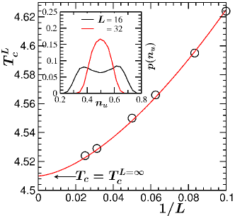
The results in Fig. 1 were obtained by using the Glauber as well as the Wolff algorithms landau ; glauber , exploiting the following facts. The fluctuation in the number of spins or particles of a particular species during simulations provides temperature dependent probability distributions for the corresponding concentration. These distribution functions are double peaked in the ordered region koyel ; landau . On the other hand, above criticality one observes single peak character. The temperature at which the crossover from double to single peak shape occurs is taken as the for a particular choice of . In the inset of Fig. 1 we show the distributions, (see caption for the details of the notation), from two different system sizes. For both the system sizes the temperature is the same. It is seen that for the larger value of there is only one peak while the distribution for the smaller system has two peaks. This is expected in the present set up and is consistent with Eq. (10). Note that the crossover between single-peak and double-peak structures occur in a continuous manner. Thus, extremely good statistics is needed to identify this. The probability distribution close to were, thus, obtained, for each , after averaging over a minimum of independent runs. Only because of this our results in the main frame of Fig. 1 are accurate, the error bars being less than the size of the symbols. can also be estimated from the locations of the maxima, with the variation of temperature, in the thermodynamic functions like susceptibility and specific heat.
To facilitate appropriate analysis of the autocorrelation data we will perform quenches from for different values of . For each , value of , to be referred to as , will be estimated. Finally, the thermodynamic limit number will be obtained from the convergence of in the limit. In addition to the -dependence, there will be other effects as well. These we will discuss in appropriate places.
In Fig. 2 we present two-dimensional cross-sections of the snapshots, taken during the evolution of both types of systems, from . For the sake of completeness we have compared the snapshots for the critical starting temperature with the ones for quenches with , i.e., from . The upper frames are for conserved order-parameter dynamics and the lower ones are for the nonconserved case. In each of the cases the structure for quenches from the critical point appears different from that for . Note that all the presented pictures are from simulations with and the results for the critical point correspond to quenches from , as mentioned above. As is well known bray_adv ; majumder_skd ; allen_cahn ; lifshitz ; huse_prb ; amar , it can be appreciated from the figure that in the nonconserved case the growth occurs much faster.

The behavior of the equal time structure factor in , for a thermodynamically large system, at criticality is expected to be fisher ; landau ; plischke
| (11) |
given that in the critical exponent (, as opposed to in ), the Fisher exponent, that characterizes the power-law factor of the critical correlation as , has a small value. Typically in most of the coarsening systems scaling in the decay of autocorrelation function [cf. Eq. (6)] starts from a reasonably large value of . By then the structure is expected to have changed from that at the beginning. Thus, the exponent ‘’ in Eq. (11) should be verified before being taken as the value of in the YRD bound for understanding of results following quenches from . Furthermore, for , one may even ask about the validity of a stable . This is related to the question whether there exists a scaling regime or the structure is continuously changing. Keeping this in mind, in Fig. 3 we present plots of versus for large enough values of and , from . Results from both the dynamics are included. In fact appears to be stable at ‘’ even though character of structure changes at large , e.g., an appearance of the Porod law bray_adv () is clearly visible that corresponds to the existence of domain boundaries. This value of , i.e., , will be used later for verifying the YRD bound.
Note here that in Fig. 3 we have presented representative results with appropriate understanding of finite-size effects and onset of scaling in the structure as well as in aging. Even though the results in Fig. 3 are from , simulating this size for long enough time, a necessity in studies of aging phenomena, in is very time consuming, particularly for the conserved dynamics. So, for aging the presented data are from smaller values of and the conclusions in the thermodynamic limit is drawn via appropriate extrapolations.
For the sake of completeness, in the inset of Fig. 3 we presented analogous results for . Here also the small behavior remains unaltered from that in the initial configuration, i.e., we have fisher . In this dimension the Porod law bray_adv demands . In the rest of the paper, all figures will contain results for only, except for the last one.

First results for are presented in Fig. 4, versus , on a log-log scale. In part (a) we have shown data for the nonconserved dynamics, by fixing the system size, for a few different values of . The observations are the following.
There exist sharp departures of the data sets from each other at large . Higher the value of the departure occurs earlier from the plot for a smaller . This is related to ‘standard’ nonequilibrium finite-size effects midya_skd ; midya_pre . With the increase of a system has less effective size available to grow or age for. This fact can be stated in the following way as well. Note that for a fixed system size the final value of is fixed. Thus, with the increase of , i.e., of , the value of the scaled variable decreases. Naturally, when the latter is chosen as abscissa variable, the finite-size effects start appearing earlier. Furthermore, even in the small region the collapse of the data set for with those for the larger values is rather poor. This, we believe, is due to the fact that in the scaling regime the structure is different yeung from the initial configuration koyel . (Also note that the scaling structure for is different from that for .) During this switch-over to the scaling behavior the extraction of is also ambiguous, due to continuous change in the structure that, thus, lacks the property of Eq. (2). If we believe that by the scaling regime has arrived (see the reasonably good collapse of data sets for and in the small regime), the corresponding decay is consistent with , a value that was predicted theoretically bray_humayun . Nevertheless, given the complexity of finite-size and other effects, further analysis is required, before arriving at a conclusion with confidence.


In part (b) of Fig. 4 we present similar results for the conserved dynamics. Here the system size is smaller than in (a). Note that due to slower dynamics in the conserved case ( for nonconserved case bray_adv ; allen_cahn , whereas for the conserved dynamics majumder_skd ; lifshitz ; huse_prb ; amar and these numbers are true irrespective bray_humayun ; humayun_bray ; nv of ) the convergence to the scaling regime has not happened even by . For the same reason the onsets of finite-size effects for different values are not so dramatically separated from each other in this case.
For both the dynamics, one gets an impression that the exponent has a tendency to increase with the increase of . The phenomenon of convergence, however, is more complex and requires systematic study involving both and . This we will perform in the rest of the paper.


Next we examine the effects of system size on the “scaling” regime. We remind the reader that there exist another type of finite-size effect related to . Due to this, with changing system size the exponent will differ in “the scaling regime” as well. Related results are presented in Fig. 5. For the sake of brevity, here, we show data only for the conserved case.
In Fig. 5 (a) we show , for different values of , versus , on a log-log scale, by fixing to . In addition to the delayed appearance of late time finite-size effects, with the increase of system size the decay exponent shows the tendency of shifting towards smaller value koyel . To pick the stable power-law regime appropriately, by discarding the finite-size affected and early transient regimes, in Fig. 5(b) we plot the instantaneous exponent midya_skd ; midya_pre ; majumder_skd ; huse_prb ; amar
| (12) |
as a function of , for a few values of with . From the flat parts we extract -dependent exponent . We have performed this exercise for multiple values of , for each type of dynamics.
An even better exercise is to extract from the plots of versus . This helps the extrapolation of to the limit, thereby elimination of any corrections, if present for small , via judicial identification of the trend of a data set. These plots are shown in Fig. 5(c). From Fig. 5(b) it was already clear that the corrections are weak in this case and so, in Fig. 5 (c) also we observe flat behavior of the relevant region and obtain the same values of . Similar procedure is followed in the nonconserved case as well. The above mentioned flat behavior in the intermediate regime confirms that there exists power-law relationship between and . The plots of Figs. 5(b) and 5(c) are expected to convey similar message. Nevertheless, the weak dependence of on , if any, will be detectable in one exercise better than the other. The exercises in these figures suggest that the corrections in the values of that may appear due to such weak dependence is within small numerical errors.
Data for , for a particular type of dynamics, when plotted versus , for multiple values of , should provide a good sense of convergence koyel . Corresponding number should be the value of for a thermodynamically large system. This exercise has been shown in Fig. 6 for both conserved (a) and nonconserved (b) dynamics. The dashed lines there are fits to the form
| (13) |
where and are constants. For both KIM and GIM, fit to each of the data sets provides value quite consistent with the others. In Fig. 7 we show analogous results for – part(a) for KIM and part(b) for GIM. Compared to Ref. koyel , these results are obtained after averaging over larger number of initial realizations. In the insets of Fig. 6 and Fig. 7, we show scaling plots of the autocorrelation function. Given that we have chosen the largest simulated system sizes, the collapse of data from different values, in each of the cases, is good. The estimated values of , obtained after averaging over the convergences of the fittings, by considering different numbers of data points for each , along with those for uncorrelated initial configurations liu_mazenko ; midya_skd ; midya_pre , are quoted in table 1. All numbers in this table are from simulation studies. For the comparison of these numbers with the YRD bound, in table 2 we have quoted the values of for starting composition of up and down spins (see caption for more details) koyel ; yeung . For the uncorrelated case it is clear that the structures are different for the conserved and nonconserved cases. For the correlated initial configurations even though the values for the two types of dynamics appear same, the overall structures are different, as expected bray_adv (see Fig. 3).
| Model | ||||
|---|---|---|---|---|
| Correlated | Uncorrelated | Correlated | Uncorrelated | |
| KIM | 0.130.02 | 3.60.2 | 0.640.05 | 7.50.4 |
| GIM | 0.140.02 | 1.320.04 | 0.570.07 | 1.690.04 |
| (0.125) | (1.29) | (0.5) | (1.67) | |
| Model | ||||
|---|---|---|---|---|
| Correlated | Uncorrelated | Correlated | Uncorrelated | |
| KIM | -1.75 (0.125) | 4 (3) | -2 (0.5) | 4 (3.5) |
| GIM | -1.75 (0.125) | 0 (1) | -2 (0.5) | 0 (1.5) |
For the sake of completeness, in table 3 we list the values of the persistence exponent bray_majumdar ; blanchard ; saikat_epjb ; saikat_pre for the two universality classes in and . Due to technical difficulty with the estimation in conserved case, for this quantity we quote only the values for the nonconserved dynamics. This table contains the values of fractal dimensionality () of the scaling structures formed by the persistent spins as well saikat_pre ; manoj_ray ; jain . From the values of the quantities presented in table 3, it is again clear that the universality for correlated and uncorrelated initial configurations are different. For the domain growth, of course, as previously mentioned, the value of does not differ between the correlated and uncorrelated initial configurations bray_humayun ; humayun_bray ; nv .
| Exponent | ||||
|---|---|---|---|---|
| Correlated | Uncorrelated | Correlated | Uncorrelated | |
| 0.035 | 0.225 | 0.105 | 0.180 | |
| 1.92 | 1.53 | 2.77 | 2.65 | |
IV Conclusion
Universality in kinetics of phase transition bray_adv is less robust compared to that in equilibrium critical phenomena fisher ; landau ; plischke . In kinetics, the classes are decided bray_adv by transport mechanism, space dimension, order-parameter symmetry and its conservation, etc. In each of these cases there can be further division into universality classes bray_humayun ; blanchard ; saikat_epjb ; saikat_pre ; koyel based on the range of spatial correlation in the initial configurations. In this paper we have examined the influence of long range correlation on the decay of order-parameter autocorrelation function, a key quantity for the study of aging phenomena zannetti ; fisher_huse in out-of-equilibrium systems, by quenching the nearest neighbor Ising model fisher ; plischke from the critical point to the ordered region. We have investigated both conserved bray_adv and nonconserved bray_adv order-parameter dynamics.
In the nonconserved case our study mimics coarsening in an uniaxial ferromagnet. On the other hand, the conserved dynamics is related to the kinetics of phase separation in solid binary mixtures. Despite difficulty due to multiple sources of finite-size effects, we have estimated the exponents for the power-law fall of the autocorrelation function rather accurately. We observe that in both the cases the decays are significantly slower than those for the quenches from perfectly random initial configurations zannetti ; fisher_huse ; liu_mazenko ; midya_skd ; midya_pre .
Even though for quenches with the values of differ significantly in the two cases, for quenches from the critical point, i.e., for , the exponents are practically same. This is irrespective of the space dimension. For the magnetic case there exist analytical prediction bray_humayun and the numbers obtained from our simulations are in reasonable agreement with the former. The source of deviations that exist may have its origin in the estimation error for as well as in the statistical error in nonequilibrium simulations. The discrepancy in may still be real given that KIM and GIM numbers from our analysis are quite close to each other.
In the literature of aging phenomena there exist lower bounds fisher_huse ; yrd for the values of . Our results for both types of dynamics are consistent with one of these bounds. This we have checked via the analysis of structure, a property that is embedded in the construction of the bound.
This work, combined with a few others midya_skd ; bray_humayun ; midya_pre ; blanchard ; saikat_epjb ; saikat_pre ; koyel , provides a near-complete information on the universality in coarsening dynamics in Ising model, involving “realistic” space dimensions, conservation property of the order parameter and spatial correlations in the initial configurations. Analogous studies in other systems should be carried out, by employing the methods used here, to obtain more complete understanding, e.g. of the influences of hydrodynamics on relaxation in out-of-equilibrium systems with long range initial correlations.
References
- (1) A.J. Bray, Adv. Phys. 51, 481 (2002).
- (2) K. Binder, in Phase Transformation of Materials, edited by R.W. Cahn, P. Haasen and E.J. Kramer (Wiley VCH, Weinheim, 1991), vol. 5. p. 405.
- (3) A. Onuki, Phase Transition Dynamics (Cambridge University Press, Cambridge, UK, 2002).
- (4) R.A.L. Jones, Soft Condensed Matter (Oxford University Press, Oxford, UK, 2002).
- (5) A.J. Bray, S.N. Majumdar and G. Schehr, Adv. Phys. 62, 225 (2013).
- (6) M. Zennetti, in Kinetics of Phase Transitions, edited by S. Puri and V. Wardhawan (CRC Press, Boca Raton, 2009).
- (7) D.S. Fisher and D.A. Huse, Phys. Rev. B 38, 373 (1988).
- (8) F. Liu and G.F. Mazenko, Phys. Rev. B 44, 9185 (1991).
- (9) C. Yeung, M. Rao and R.C. Desai, Phys. Rev. E 53, 3073 (1996).
- (10) M. Henkel, A. Picone and M. Pleimling, Europhys. Lett. 68, 191 (2004).
- (11) C. Yeung and D. Jashnow, Phys. Rev. B 42, 10523 (1990).
- (12) F. Corberi, E. Lippiello and M. Zannetti, Phys. Rev. E 74, 041106 (2006).
- (13) E. Lorenz and W. Janke, Europhys. Lett. 77, 10003 (2007).
- (14) J. Midya, S. Majumder and S.K. Das, J. Phys. Condens. Matter 26, 452202 (2014).
- (15) S. Paul and S.K. Das, Phys. Rev. E 96, 012105 (2017).
- (16) S. Roy, A. Bera, S. Majumder and S.K. Das, Soft Matter 15 4743 (2019).
- (17) A.J. Bray, K. Humayun and T.J. Newman, Phys. Rev. B 43, 3699 (1991).
- (18) J. Midya, S. Majumder and S.K. Das, Phys. Rev. E 92, 022124 (2015).
- (19) E. Lippiello, A. Mukherjee, S. Puri and M. Zannetti, Europhys. Lett. 90, 46006 (2010).
- (20) F. Corberi and R. Villavicencio-Sanchez, Phys. Rev. E 93, 052105 (2016).
- (21) K. Humayun and A.J. Bray, J. Phys. A: Math. Gen. 24, 1915 (1991).
- (22) S.B. Dutta, J. Phys. A: Math. Theor. 41, 395002 (2008).
- (23) T. Blanchard, L.F. Cugliandolo and M. Picco, J. Stat. Mech.: Theor. Expt. P12021 (2014).
- (24) S. Chakraborty and S.K. Das, Eur. Phys. J. B 88, 160 (2015).
- (25) S. Chakraborty and S.K. Das, Phys. Rev. E 93, 032139 (2016).
- (26) S.K. Das, K. Das, N. Vadakkayil, S. Chakraborty and S. Paul, J. Phys. Condens. Matter, 32, 184005 (2020).
- (27) M.E. Fisher, Rep. Prog. Phys. 30, 615 (1967).
- (28) J.F. Marko and G.T. Barkema, Phys. Rev. E 52, 2522 (1995).
- (29) M.E. Fisher and M.N. Barber, Phys. Rev. Lett. 28, 1516 (1972).
- (30) D.W. Heermann, L. Yixue and K. Binder, Physica A 230, 132 (1996).
- (31) S. Majumder and S.K. Das, Phys. Rev. E 84, 021110 (2011).
- (32) C. Yeung, Phys. Rev. Lett. 61, 1135 (1988).
- (33) K. Binder and D.W. Heermann, Monte Carlo Simulations in Statistical Physics (Springer, Switzerland, 2019).
- (34) D.P. Landau and K. Binder, A Guide to Mote Carlo Simulations in Statistical Physics (Cambridge University Press, Cambridge, 2009).
- (35) D. Frenkel and B. Smit, Understanding Molecular Simulations: From Algorithms to Applications (Academic Press, San Diego, 2002).
- (36) K. Kawasaki, in Phase Transition and Critical Phenomena, edited by C. Domb and M.S. Green (Academic, New York, 1972), Vol. 2, p. 443.
- (37) R.J. Glauber, J. Math. Phys. 4, 294 (1963).
- (38) U. Wolff, Phys. Rev. Lett. 62, 361 (1989).
- (39) P.C. Hohenberg and B.I. Halperin, Rev. Mod. Phys. 49, 435 (1977).
- (40) S.K. Das, S. Roy, S. Majumder and S. Ahmad, Europhy. Lett. 97, 66006 (2012).
- (41) E. Luijiten, M.E. Fisher and A.Z. Panagiotopoulos, Phys. Rev. Lett. 88, 185701 (2002).
- (42) S.K. Das, Y.C. Kim and M.E. Fisher, Phys. Rev. Lett. 107, 215701 (2011).
- (43) S. Roy and S.K. Das, Europhys. Lett. 94, 36001 (2011).
- (44) J. Midya and S.K. Das, J. Chem. Phys. 146, 044503 (2017).
- (45) M. Plischke and B. Bergersen, Equilibrium Statistical Physics (World Scientific, London, 2005).
- (46) S.M. Allen and J.W. Cahn, Acta Metall. 27, 1085 (1979).
- (47) I.M. Lifshitz and V.V. Slyozov, J. Phys. Chem. Solids 19, 35 (1961).
- (48) D.A. Huse, Phys. Rev. B 34, 7845 (1986).
- (49) J.G. Amar, F.E. Sullivan and R.D. Mountain, Phys. Rev. B 37, 196 (1988).
- (50) N. Vadakkayil, K. Das, S. Paul and S.K. Das, to be published.
- (51) G. Manoj and P. Ray, J. Phys. A 33, 5489 (2000).
- (52) S. Jain and H. Flynn, J. Phys. A 33, 8383 (2000).