Agent based simulators for epidemic modelling: Simulating larger models using smaller ones
Abstract
Agent-based simulators (ABS) are a popular epidemiological modelling tool to study the impact of various non-pharmaceutical interventions in managing an epidemic in a city (or a region). They provide the flexibility to accurately model a heterogeneous population with time and location varying, person-specific interactions as well as detailed governmental mobility restrictions. Typically, for accuracy, each person is modelled separately. This however may make computational time prohibitive when the city population and the simulated time is large. In this paper, we dig deeper into the underlying probabilistic structure of a generic, locally detailed ABS for epidemiology to arrive at modifications that allow smaller models (models with less number of agents) to give accurate statistics for larger ones, thus substantially speeding up the simulation. We observe that simply considering a smaller aggregate model and scaling up the output leads to inaccuracies. We exploit the observation that in the initial disease spread phase, the starting infections create a family tree of infected individuals more-or-less independent of the other trees and are modelled well as a multi-type super-critical branching process. Further, although this branching process grows exponentially, the relative proportions amongst the population types stabilise quickly. Once enough people have been infected, the future evolution of the epidemic is closely approximated by its mean field limit with a random starting state. We build upon these insights to develop a shifted, scaled and restart-based algorithm that accurately evaluates the ABS’s performance using a much smaller model while carefully reducing the bias that may otherwise arise. We apply our algorithm for Covid-19 epidemic in a city and theoretically support the proposed algorithm through an asymptotic analysis where the population size increases to infinity. We develop nuanced coupling based arguments to show that the epidemic process is close to the branching process early on in the simulation.
1 Introduction
Agent-based simulators (ABS) are a popular tool in epidemiology (See [12], [5]). In this paper we focus on ABS used to model epidemics such as Covid-19 in cities and we illustrate our methodological contributions through the use of ABS for modelling Covid evolution in the city of Mumbai. As is apparent from the paper, the underlying ideas are valid more generally for any epidemic in a large city that may have an initial exponential growth phase that tapers down when sufficient population is infected (See [4], [7]).
As is well known, in an ABS in epidemic modelling of a city, a synthetic copy of it is constructed on a computer that captures the population interaction spaces and detailed disease spread as well as disease spreading interactions as they evolve in time. Typically, each individual in the city is modelled as an agent, so that total number of agents equal the total city population. The constructed individuals reside in homes, children may go to schools, adults may go to work. Individuals also engage with each other in community spaces (to capture interactions in marketplaces, restaurants, public transport, and other public places). Homes, workplaces, schools sizes and locations and individuals associated with them, their gender and age, are created to match the city census data and are distributed to match its geography. Government policies, such as partial, location specific lockdowns for small periods of time, case isolation of the infected and home quarantine of their close contacts, closure of schools and colleges, partial openings of workplaces, etc. lead to mobility reduction and are easily modelled. Similarly, variable compliance behaviour in different segments of the population that further changes with time, is easily captured in an ABS. Further, it is easy to introduce new variants as they emerge, the individual vaccination status, as well as the protection offered by the vaccines against different variants as a function of the evolving state of the epidemic and individual characteristics, such as age, density of individual’s interactions, etc (see [13]). Thus, this microscopic level modelling flexibility allows ABS to become an effective strategic and operational tool to manage and control the the disease spread. See [5] for an ABS used for UK and USA related studies specific to COVID-19, [8] for a COVID-19 study on Sweden, [1], [13] for a study on Bangalore and Mumbai in India. See, e.g., [9] and [12] for an overview of different agent-based models.
Key drawback: However, when a reasonably large population is simulated, especially over a long time horizon, an ABS can take huge computational time and this is its key drawback. This becomes particularly prohibitive when multiple runs are needed using different parameters. For instance, any predictive analysis involves simulating a large number of scenarios to provide a comprehensive view of potential future sample paths. In model calibration, the key parameters such as transmission rates, infectiousness of new variants are fit to the observed infection data over relevant time horizons, requiring many computationally demanding simulations.
Key contributions: We develop a shift-scale-restart algorithm (described later) that carefully exploits the closeness of the underlying infection process (process of number infected of each type at each time), first to a multi-type super critical branching process, and then, suitably normalised, to the mean field limit of the infection process, so that the output from the smaller model accurately matches the output from the larger one. Essentially, both the smaller and the larger model, with identical initial conditions of small number of infections evolve similarly in the early days of the infection growth. Interestingly, in a super-critical branching process, while the number of infections grows exponentially, the proportions of the different types infected quickly stabilises, and this allows us to shift a scaled path from a smaller model to a later time with negligible change in the underlying distribution. Therefore, once there are enough infections in the system, output from the smaller model, when scaled, matches that from the larger model at a later ‘shifted’ time. This shifting and scaling of the paths from the smaller model does a good job of representing output from the larger model when there are no interventions to the system. However, realistically, government intervenes and population mobility behaviour changes with increasing infections. To get the timings of these interventions right, we restart the smaller model and synchronise the timings of interventions in the shifted and scaled path to the actual timings in the original path of the larger model.
We present numerical results where our strategy is implemented on a model for Mumbai with 12.8 million population that realistically captures interactions at home, school, workplace and community as well as mobility restrictions through interventions such as lockdown, home quarantine, case isolation, schools closed, limited attendance at workplaces, etc. Using our approach, we more or less exactly replicate 12.8 million population model for Mumbai with all its complexities, using only 1 million people model, providing an almost 12.8 times speed-up. We numerically observe similar results with a smaller half-million population model, although further reduction leads to increase in errors as the branching process phase is very small and mean field approximations break down. Mumbai is a densely populated city. To check for validity of our approach to less dense cities, we reduce the parameters that capture interactions and numerically observe that the proposed approach works well even in substantially sparser cities.
Further, we provide theoretical support for the proposed approach through an asymptotic analysis where the population size increases to infinity. We show that early on till time , where is the exponential epidemic growth rate in early stages and denotes the number exposed at time zero, the epidemic process is well approximated by an associated branching process. Our analysis relies on developing a nuanced coupling between the epidemic and the branching process during this period. Then, after time for any , and large , we show that the epidemic process is closely approximated by its mean field limit that can be seen to follow a large dimensional discretized ODE. While, our simulation model allows each person’s state to lie in an uncountable state space, our theoretical analysis is conducted under somewhat simpler finite state assumptions, that subsumes general compartmental models.
In the Appendix we also identify the behaviour of simple compartmental models such as susceptible-infected and recovered (SIR) and some generalisations in the early branching process phase before it is governed by the ODE (see Appendix B).
Structure of remaining paper: To illustrate the key ideas practically, we first show the implementation of our algorithm on a realistic model of Mumbai in Section 2. Then in Section 3, we briefly summarise our agent based simulator. In Section 4 we spell out the shift-scale-restart algorithm. We provide theoretical asymptotic analysis supporting the efficacy of the proposed algorithm in Section 5. We first conduct our analysis in a simpler set-up where the coupling between the epidemic and the branching process and the related analysis is easier. A more general analysis, and a more intricate coupling is analysed in the Appendix D. Section 5 is accompanied with brief proof sketches of the results while the details are presented in Appendix C. In Section 6 we demonstrate the performance of our algorithm for less dense cities and smaller half million and one lakh models. In section 7 we conclude.
2 Speeding up ABS: The big picture
A naive approach to speed up the ABS maybe to use a representative smaller population model and scale up the results. Thus, for instance, while a realistic model for Mumbai city may have 12.8 million agents (see [11]), we may construct a sparser Mumbai city having, say, a million agents, that matches the bigger model in essential features, so that, roughly speaking, in the two models each infectious person contributes the same total infection rate to all susceptibles at each time. The output numbers from the smaller model may be scaled by a factor of 12.8 to estimate the output from the larger model. We observe, somewhat remarkably, that this naive approach is actually accurate if the initial seed infections in the smaller model (and hence also the larger model) are large, say, of the order of thousands, and are identically distributed in both the smaller and the larger model (see Figure 3 where the number exposed are plotted under a counter-factual no interventions scenario. The comparative statements hold equally well for other statistics such as the number infected, hospitalised, in ICUs and deceased). The rationale is that in this setting both the smaller and the larger model have sufficient infections so that the proportion of the infected population in both the models well-approximate their identical mean field limits.


However, modelling initial randomness in the disease spread is important for reasons including ascertaining the distribution of when and where an outbreak may be initiated, the probability that some of the initial infection clusters die-down, getting an accurate distribution of geographical spread of infection over time, capturing the intensity of any sample path (the random variable in the associated branching process, described in Theorem 5.2), etc. These are typically captured by setting the initial infections to a small number, say, around a hundred, and the model is initiated at a well chosen time (see [1]). In such settings, we observe that the scaled output from the smaller model (with proportionately lesser initial infections) is noisy and biased so that the simple scaling fix no longer works (see Figure 3. In Appendix E, we explain in a simple setting why the scaled smaller model is biased and reports lower number of infections compared to the larger model in the early infection spread phase).
Additionally, we observe that in the early days of the infection, the smaller and the larger model with the same number of initial infections, similarly clustered, behave more or less identically (see Figure 3), so that the smaller model with the unscaled number of initial seed infections provides an accurate approximation to the larger one. Here again in the early phase in the two models, each infectious person contributes roughly the same total infection rate to susceptibles at home, workplace and community. Probabilistically this is true because early on, both the models closely approximate an identical multi-type branching process. Shift-scale-restart algorithm outlined in Section 4 exploits these observations to speed up the simulator. We briefly describe it below.
Fixing ideas: Suppose that for Mumbai with an estimated population of million, a million agent model is seeded with randomly distributed infections on day zero. To get the statistics of interest such as expected hospitalisations and fatalities over time, instead of running the million agent model, we start a million agent model seeded with similarly randomly distributed infections at day zero and generate a complete path for the requisite duration. To get the statistics for the larger model, we first observe that under the no-intervention scenario, the output of the smaller model more or less exactly matches that of the larger model for around first days (Figure 5). As our analysis in Section 5 suggests, the two models closely approximate the associated branching process till time where denotes the population of the smaller model and equals 1 million, denotes the number exposed at time zero and equals 100, and denotes the exponential growth rate in the early fatalities and is estimated from fatality data to equal 1.21. The quantity is estimated to equal 34.5 suggesting that both are close to the underlying branching process around day 35. After this initial period of around days, the city has an average of thousand infections. We then determine the day when the city had thousand infections. This turns out to be day in our example. We take the path from day 21.5 onwards, scale it by a factor of 12.8, and concatenate it to the original path starting at day . Theoretical justification for this time shift comes from the branching process theory, where while a super-critical multi-type branching process can be seen to grow exponentially with a sample path dependent intensity, the relative proportions amongst types along each sample path stabilise fairly quickly and become more-or-less stationary (see Theorem 5.2). This shifted and scaled output after 35 days matches that of the larger model remarkably well. See Figure 5 where the generated infections from the larger million model and the shifted and scaled smaller million model are compared. The choice of day 35 is not critical above. Similar results would be achieved if we used lesser, as low as 25 days in the original model.
In a realistic setting, administration may intervene once the reported cases begin to grow. Suppose in the above example, an intervention happens on day 40. (This is reasonable, as in modelling Mumbai, our calibration exercise had set the day zero to February 13, 2020 (see, [11]), the resulting infections and reported cases reached worrying levels around the second week of March. Restrictions in the city were imposed around March 20, 2020.) In that case, the shifted and scaled path from the day 21.5 would need to have the restrictions imposed on day 26.5 (so that it approximates day 40 for the larger model). We achieve this by using the first generated a path till day 35, computing the appropriate scaled path time (21.5 days, in this case), and then, using common random numbers, restarting an identical path from time zero that has restrictions imposed from day 26.5. This path is scaled from day 21.5 onwards and concatenated to the original path at day 35. In Section 5 we note that the restarted path need not use common random numbers (see Remark 1). Even if it is generated independently, we get very similar output.


Figure 5 compares the number exposed in a 12.8 million Mumbai city simulation (in no intervention scenario) with the estimates from the shift-scale-restart algorithm applied to the smaller 1 million city. Numerical parameters for the no-intervention scenario for Mumbai are described in Appendix F. Figure 5 compares the exposed population process for the 12.8 million population Mumbai model with the smaller 1 million one as per our algorithm under realistic interventions (lockdown, case isolation, home quarantine, masking etc.) introduced at realistic times, as implemented in [1] using similar parameters, for 250 days. In this experiment, smaller and larger city evolves similarly till day 22. Intervention is at day 33, therefore smaller city is restarted with intervention at day 22.5 and scaled estimates from day 11.5 of the restarted simulation are appended at day 22 of the initial run (i.e. shifted by 10.5 days). We see that the smaller model faithfully replicates the larger one with negligible error. Similar results hold for other health statistics such as the number hospitalised and the number of cumulative fatalities, and for larger models that include variants (see Appendix A).
3 Agent Based Simulator
We informally and briefly describe the main drivers of the dynamics in our ABS model. A more detailed discussion can be seen in [1].
The model consists of individuals and various interaction spaces such as households, schools, workplaces and community spaces. Infected individuals interact with susceptible individuals in these interaction spaces. The number of individuals living in a household, their age, whether they go to school or work or neither, schools and workplaces size and composition all have distributions that may be set to match the available data. The model proceeds in discrete time steps of constant width (six hours in our set-up). At a well chosen time zero, a small number of individuals can be set to either exposed, asymptomatic, or symptomatic states, to seed the infection. At each time , an infection rate is computed for each susceptible individual based on its interactions with other infected individuals in different interaction spaces (households, schools, workplaces and community). In the next time, each susceptible individual moves to the exposed state with probability , independently of all other events. Further, disease may progress independently in the interval for the population already afflicted by the virus. The probabilistic dynamics of disease progression as well as implementation of public health safety measures are briefly summarized below under simplified assumptions (underlying model is similar to that in [5] and [1]). Simulation time is then incremented to , and the state of each individual is updated to reflect the new exposures, changes to infectiousness, hospitalisations, recoveries, quarantines, etc., during the period to . The overall process repeats incrementally until the end of the simulation time.
3.1 Computing
A susceptible individual at any time receives a total infection rate which is sum of the infection rates (from home), (from school), (from workplace) and (from community) coming in from infected individuals in respective interaction spaces of individual .
Briefly, the transmission rate () of virus by an infected individual in each interaction space is the expected number of eventful (infection spreading) contact opportunities with all the individuals in that interaction space. It accounts for the combined effect of frequency of meetings and the probability of infection spread during each meeting. An infected individual can transmit the virus in the infective (pre-symptomatic or asymptomatic stage) or in the symptomatic stage. Each individual has two other parameters: a severity variable (individual attendance in school and workplace depends on the severity of disease) and a relative infectiousness variable, virus transmission is related linearly to this. Both bring in heterogeneity to the model.
Specifically, let when an individual can transmit the virus at time , otherwise. To keep notation simple, we avoid describing the details of individual infectiousness, severity, age dependent mobility and community density factor (see [1] for details). Let , , , and denote the transmission coefficients at home, school, workplace and community spaces, respectively. A susceptible individual who belongs to home , school , workplace and community space sees the following infection rates at time in different interaction spaces:
is the average transmission rate coming in to individual from each infected individual in his home.
and are also computed similarly based on infected individuals in respective interaction spaces of the individual .
Different wards in the city constitute different communities. In our numerical experiments for Mumbai, since slums form more than half the population and are extremely dense, we further divide each ward into slum and non-slum community. To compute infection rate to an individual from the community, we first compute the infection rate for each community at a given time . This is set to the sum of transmission rate from all the infected individuals of the community assigned a weight that is proportional to the strictly decreasing function of the distance between the individual and the community centre. Specifically,
| (1) |
where is a distance kernel that is strictly decreasing in . As in [6], one may select and for appropriately chosen non-negative constants and . Note that is dominated by and it equals only when everyone in the community is infected.
The infection rate seen by an individual in community is set to sum of the community infection rates from different communities of the city multiplied with weights that are again proportional to the strictly decreasing function of the distance between the two communities. This quantity is further adjusted for the distance between individual and its community centre. Specifically,
| (2) |
Again observe that, if , then . Further, an age dependent factor determining the mobility of the individuals in the community may also be accounted in (see [1]).
3.2 Disease progression
In the numerical experiments, the disease progression model is based on COVID-19 progression as described in [16] and [5]. An individual may have one of the following states: susceptible, exposed, infective (pre-symptomatic or asymptomatic), recovered, symptomatic, hospitalised, critical, or deceased. Briefly, an individual after getting exposed to the virus at some time observes an incubation period which is random with a Gamma distribution. Individuals are infectious for an exponentially distributed period. This covers both presymptomatic transmission and possible asymptomatic transmission. We assume that a third of the patients recover, these are the asymptomatic patients; the remaining develop symptoms. Individuals either recover or move to the hospital after a random duration that is exponentially distributed (see Appendix F for model input data details). The probability that an individual recovers depends on the individual’s age. While hospitalised individuals may continue to be infectious, they are assumed to be sufficiently isolated, and hence do not further contribute to the spread of the infection. Further progression of hospitalised individuals to critical care and further to fatality is also age dependent.
3.3 Public health safety measures (PHSMs)
We introduce methodologies to model different PHSMs (or Interventions) such as lockdowns, home quarantine, case isolation, social distancing of elderly population, mobility restrictions, masks etc. Table 7 in Appendix F summarizes some of the key interventions implemented. The PHSM’s mentioned above when implemented put some restrictions on the individual’s mobility. However, it is often the case that when several restrictions are in place, only a fraction of the population comply with these restrictions. Therefore, we restrict the movement of only the individuals in the compliant fraction of households in the city.
4 Shift-scale-restart algorithm
Let denote the initial distribution of the infected population at time zero in our model with population and let the simulation run for a total of time units. E.g., for Mumbai at a suitably chosen time 0, we select people at random from the non-slum population and mark them as exposed. (Since initially the infection came from international travellers flying into Mumbai, it is reasonable to assume that most of them were residing in non-slums). Algorithm 1 summarises the simulation dynamics.
Scaling the model: For , , let be the number of individuals in the larger city, and in the smaller city. Roughly speaking, the larger city has times more homes, schools and workplaces compared to the smaller city. The joint distribution of people in homes, schools or workplaces is unchanged, and transmission rates , , and are unchanged (recall that each transmission rate of an infected individual in each interaction space is the expected number of infection spreading contact opportunities with all the individuals in that interaction space. It accounts for the combined effect of frequency of meetings and the probability of infection spread during each meeting).
When we initiate both the larger as well as the smaller city with a same few and well spread infections, the disease spreads similarly in homes, schools and workplaces. To understand the disease spread through communities, for simplicity assume that there is a single community. It is easy to see that each susceptible person sees approximately times the community infection rate in the larger city compared to the smaller city. On the other hand, the larger city has times more susceptible population. This is true even when there are more communities and for a general distance function (see Section 3.1 for role of in community infection rates). Therefore, early on in the simulation, the total number getting infected through communities is also essentially identical between the larger and the smaller city, and the infection process in the two cities evolves very similarly.
Let denote the time till the two cities evolve essentially identically (as seen empirically and suggested by theoretical analysis, this is close to for . Here for any and denotes the initial infection exponential growth rate.)
In this setting, we propose that a shift and scale Algorithm 2, that builds upon Algorithm 1, be applied to the smaller city to generate output that resembles the larger city. Algorithm 2 is graphically illustrated in Figure 7.
In a realistic scenario, as the infection spreads, the administration will intervene and impose mobility restrictions. Thus, our simulation adjustments to the small city need to account for the timings of these interventions accurately. Let denote the first intervention time (e.g., lockdown; typically after time for small ). Let . We need to restart our simulation to ensure that the shift and scaled path incorporates the intervention at the correct time. The Algorithm 3 achieves this and is graphically illustrated in Figure 7.
As we see empirically, and as is suggested by Proposition 5.1, in Algorithm 3, evolution of the infection process after time , given the state at that time, is more or less deterministic (even though the process may be close to the associated branching process at this time).


5 Asymptotic Analysis
In SSR algorithm, theoretical justification is needed for the fact that early on in the small city simulation, we could take a path at one time period, scale it, and stitch it to the path at another appropriately chosen time period, to accurately generate a path for the larger city. We provide this through an asymptotic analysis as the city population increases to infinity. We prove that in the initial disease spread phase, the epidemic process is close to a multi-type super-critical branching process by coupling the two processes. Further we prove that, once enough people have been infected, the future evolution of the epidemic is closely approximated by its mean field limit with a random starting state.
Recall that the synthetic model of the city is generated in two steps. We first instantiate the individuals, households, schools, workplaces and communities using the population level statistics of the demographic profile of the city. Secondly, these individuals are randomly assigned to households, schools etc. As a result, the graph of the population in the whole city might be connected to each other through schools, workplaces and homes (apart from being connected through community). As we also discuss later, in our asymptotic analysis the number of homes, schools and workplaces increase to infinity with . This implies that the state space of the population network will go to as , making the analysis significantly more complex.
For the ease of analysis, we assume that the state of the city takes fixed, finitely many values as . Specifically, we assume that the city contains many groups of individuals, each group of fixed finite population. An individual in a group interacts with another group only through community so an infectious individual in one group can infect a person in another group only through community interactions. All the other interactions (home, school, workplace) of individuals are within a group. Each group may be thought as comprising many households where children may go to schools and adults may go to work within the same group. This group structure remedies the problem of infinite state space, as a group of finite size can only have finitely many types (considering different types of individuals and their networks). Additionally, it was experimentally observed that for large group sizes, the results from the actual simulation model and similar group structured model were very close.
Even though the group structure makes the state space finite, the analysis involves nuanced arguments for coupling the epidemic and branching processes. To keep the discussion simple and intuitive, in the main body, we consider a simpler model with only one individual in a group thereby ignoring the interaction spaces of homes, workplaces and schools. For groups of size greater than 1, the analysis using the group structure involves an intricate coupling argument and is presented in the Appendix D.
Table 1, elaborates the differences between the simulation model and the two models analysed asymptotically - the intermediate group-structure model and the simplified model with groups of size 1.
| City | Intermediate | Simplified | ||
| simulation | model for | model for | Remarks | |
| model | analysis | analysis | ||
| Presence of | Intermediate model: Population is divided into | |||
| homes, schools | Yes | Yes | No | groups. All the home, school and workplace |
| and workplaces | interactions of an individual are within a group. | |||
| Number of | Multiple | 1 | 1 | Intermediate, simplified model: Extension to |
| communities | multiple communities is straightforward. | |||
| Distance of an | ||||
| individual from | Continuous | Constant | Constant | Intermediate, simplified model: Extension to |
| community | multiple distances is straightforward. | |||
| center | ||||
| Not | Intermediate model: Single group | |||
| Groups | applicable | Yes | Yes | type is considered. Extension to |
| Multiple group types is straightforward. |
We briefly review the standard multi-type branching process in Section 5.1. In the following analysis, we define an epidemic process in Section 5.2. Further, we define a multi-type super-critical branching process tailored to the epidemic process in Section 5.3. We describe the coupling between the two processes in Section 5.4. We then state the results demonstrating the closeness of the epidemic and the branching process in the early disease spread phase in Section 5.5. The results demonstrating the closeness of the epidemic process to its mean field limit once the epidemic process has grown are given in Section 5.6.
5.1 Supercritical multi-type branching process review
In this section, we first define a multi-type branching process and state a key result associated with a super critical multi-type branching process and an assumption outlining a set of sufficient conditions for it to hold. See [2] for details.
Let be a dimension vector denoting the multi-type branching process at time , where . Component of denotes the number of individuals of type at time . As is well known, in a multi-type branching process, at the end of each time period an individual may give birth to children of different types and itself dies (it may reincarnate as a child of same or different type). The number of children each individual of type gives birth to is independent and identically distributed. Therefore, multi-type branching process is a Markov chain . Suppose , then is sum of independent offsprings of type parents, independent offsprings type parents, and so on. Thus, is sum of independent random vectors in .
Consider a matrix such that , that is expected number of type offsprings of a single type individual in one time period. Then,
Recall that the Perron Frobenius eigenvalue of a non-negative irreducible matrix (a non-negative square matrix is irreducible if there exists an integer such that all entries of are strictly positive) is its largest eigenvalue in absolute value, and can be seen to be positive. The following assumption is standard in multi-type branching process theory (see [2]).
Assumption 1.
is irreducible and its Perron Frobenius eigenvalue Furthermore,
for all .
By we denote that the sequence of random variables converges to in probability as . Theorem 4 below is well known (see [2]).
Suppose that Assumption 1 holds. Then, corresponding to eigenvalue , there exist strictly positive right and left eigenvectors of , and such that and .
Theorem 5.1.
Under Assumption 1,
Furthermore,
| (3) |
where is a non-negative random variable such that and for all . Let . Then, for any and for all
| (4) |
5.2 Epidemic process dynamics
Notation: The city comprises of individuals and our interest is in analyzing the city asymptotically as .
-
•
An individual at any time can be in one of the following disease states: Susceptible, exposed, infective, symptomatic, hospitalised, critical, dead or recovered. Individuals are infectious only in infective or symptomatic states. Denote all the disease states by . For simplicity, we ignore possible reinfections, although incorporating them would not alter our conclusions.
-
•
Each individual has some characteristics that are assumed to remain unchanged throughout the epidemic regardless of it’s disease state. These include individual’s age group, disease progression profile (e.g., some may be more infectious than others), community transmission rates (e.g., individuals living in congested slums may be modelled to have higher transmission rates), mobility in the community (e.g., elder population may travel less to the community compared to the working age population). We assume that set of all possible individual characteristics are finite, and denote them by . Let , for , denote the total number of individuals with characteristic in system , and set for all . We assume that is independent of as .
-
•
Hence, each individual at any time may be classified by a type , where denotes the individual characteristic and the disease state. Let denote the set of all types.
-
•
Let denote all the types with susceptible disease state. Hence, denote the types where individuals are already affected (that is, they have been exposed to the disease at some point in the past). Let .
-
•
Denote the number of individuals of type at time by and set . Then, .
-
•
Let denote the total number of affected individuals in the system at or before time .
Dynamics: At time zero, for each , is initialised by setting a suitably selected small and fixed number of people randomly from some distribution and assigning them to the exposed state. All others are set as susceptible. The distribution is assumed to be independent of so we can set for all N.
Given , is arrived at through two mechanisms. (For the ease of notation we will set .) i) Infectious individuals at time who make Poisson distributed infectious contacts with the rest of the population moving the contacted susceptible population to exposed state, and ii) through population already affected moving further along in their disease state. Specifically,
-
•
We assume that an infectious individual with characteristic spreads the disease in the community with transmission rate . Thus, the total number of infectious contacts it makes with all the individuals (both susceptible and affected) in one time step is Poisson distributed with rate . The individuals contacted are selected randomly and an individual with characteristic is selected with probability proportional to (independent of ). helps model biases such as an individuals living in a dense region are more likely to infect other individuals living in the same dense region. As a normalisation, set .
-
•
Once the number of infectious contacts for a particular characteristic have been generated, each contact is made with an individual selected uniformly at random from all the individuals with characteristic .
-
•
If an already affected individual has one or more contact from an infectious individual, its type remains unchanged. On the other hand, if a susceptible individual has at least one contact from any infectious individual, it gets exposed at time . Each susceptible individual with characteristic who gets exposed at time , increments by 1. A susceptible individual that has no contact with an infectious individual remains susceptible in the next time period.
-
•
Once an individual gets exposed, its disease progression is independent of all the other individuals and depends only on its characteristics, that is, the disease progression profile of the characteristic class the individual belongs to. The waiting time in each state (except susceptible, dead and recovered) is assumed to be geometrically distributed. Transition to symptomatic, hospitalised, critical, dead or recovered state happens with respective characteristic (disease progression profile) dependent transition probabilities. Thus, an individual of type , some disease state other than susceptible, at time transitions to some other state at time with the transition probability in one time step. The probability is independent of time and . If the transition happens, is decreased by 1 and is increased by 1. Observe that if characteristic of types and is different.
5.3 Associated branching process dynamics
For each , let , where denote the number of individuals of at time in the branching process.
Dynamics: At time zero . Given , we arrive at as follows:
-
•
At time , every infectious individual of type , for all , gives birth to independent Poisson distributed offspring of type at time with rate for each . is increased accordingly.
-
•
Once an individual gets exposed, disease progression of the individual has same transition probabilities as in each epidemic process. An individual of type , that is, in disease state other than susceptible at time , transitions to some other disease state at time with probability . If the transition happens, is decreased by 1 and is increased by 1.
Let denote the total number of offsprings generated by time in the branching process.
The expected offsprings matrix for : Let each entry of denote the expected number of type offspring of a single type individual in one time step. Let denote all the types with the disease states that are infectious or may become infectious in subsequent time steps (that is, types with disease state either exposed, infective or symptomatic). Let denote its complement. Individuals in do not contribute to community infection. Let denote all the types with the disease states that are infectious (that is infective or symptomatic state). Let denote , that is, the set of all the types corresponding to exposed individuals. Let .
As described above, an individual of type , may give birth to other exposed individuals if it is infectious, and/or may itself transition to some other type in one time step. Then, can be written as,
| (5) | ||||
It follows that
| (6) |
Theorem 5.2 for multi-type branching processes holds under a standard assumption that the expected offspring matrix is irreducible (for more details, see Appendix 5.1). However, as defined in (5) is not irreducible. Lemma 5.1 below sheds further light on the structure of . Theorem 5.2 observes that standard conclusions continue to hold for the branching process associated with epidemic processes .
For any matrix , let denote its spectral radius, that is, the maximum of the absolute values of all its eigenvalues. Henceforth, we assume that in all subsequent analysis.
Lemma 5.1.
There exist matrices , and such that
where is irreducible. Further, .
As defined in Lemma 5.1 is irreducible, its Perron Frobenius eigenvalue is equal to its spectral radius .
Theorem 5.2.
Spectral radius of is equal to the spectral radius of , that is, . Furthermore, is a unique eigenvalue of with maximum absolute value and where and are the strictly positive right and left eigenvectors of corresponding to eigenvalue such that and .
In addition, as , where is a non-negative random variable such that iff for some and for all . Also, let as . Then, for any and for all ,
Observe that for all holds because the offsprings for our branching process have a Poisson distribution.
Proof sketch for Lemma 5.1 and Theorem 5.2: Lemma 5.1 follows by observing that: 1) correspond to types of individuals with disease states that are infectious or may become infectious. These types may give birth to exposed individuals of each characteristic in subsequent time steps and is therefore irreducible. 2) As any individual in hospitalised, critical, dead or recovered disease states neither transitions nor gives birth to offspring in exposed, infective or symptomatic disease states, therefore, we have submatrix in . 3) corresponds to type of individuals that do not contribute to any infections in the city. In addition, these individuals either transition to the next disease state or remain in the same disease state with positive probability. This results in all the eigenvalues of C being less than or equal to 1. Theorem 5.2 then follows easily by combining the Lemma 5.1 and the standard results for branching processes. For detailed proof, see Appendix C.1 and C.2.
5.4 Coupling epidemic and branching process
-
•
Recall that at time zero, . We couple each exposed individual of each type in the epidemic process to an exposed individual of the same type in the branching process at time zero.
-
•
The coupled individuals in each of these processes follow the same disease progression (using same randomness) and stay coupled throughout the simulation.
-
•
Further, when infectious, they generate identical Poisson number of contacts (in epidemic process) and offsprings (in branching process). Specifically, when a coupled individual with characteristic is infectious, the number of contacts it makes in a time step with all the individuals with characteristic in epidemic process is Poisson distributed with rate . This equals the offsprings generated by the corresponding coupled individual in the branching process where the offsprings are with characteristic and are of type .
-
•
In epidemic process, each contact is made with an individual randomly selected from the population with the same characteristic. If a contact is with a susceptible person, then that person is marked exposed in the next time period and is coupled with the corresponding person in the branching process.
-
•
On the other hand, if in epidemic process, a new contact is with an already affected individual, then this does not result in any person getting exposed so that the corresponding offspring in the branching process is uncoupled. The descendants of uncoupled individuals in the branching process are also uncoupled. In our analysis, we will show that such uncoupled individuals in the branching process vis-a-vis epidemic process are a negligible fraction of the coupled individuals till time for large , where recall that and and denotes the exponential growth rate of the branching process.
Denote the new uncoupled individuals born from the coupled individuals in branching process at each time by (referred to as “ghost individuals”). As mentioned earlier, these and their descendants remain uncoupled to epidemic system . Let denote all the descendants of (ghost individuals born at time ) after time steps, i.e. at time .
5.5 The initial branching process phase
Following result shows that epidemic process is close to the multi-type branching process till time .
Theorem 5.3.
As , for all ,
| (7) |
| (8) |
Result (7) was earlier shown for SIR setting in [3]. We extend this result to general models and also prove the result (8) in this more general setting.
Lemma 5.2.
For all , and for some ,
Proof sketch for Theorem 8 and Lemma 5.2: For all , is bounded from above by (total number of uncoupled individuals till time ). Recall that the ghost individuals () arise as a result of the infectious individuals in epidemic process making contact with already affected individuals and is related to their product. Further, infectious individuals are upper bounded in no. by affected individuals and hence it can easily be shown that for some and any . Further, from coupling we have for all . Inequality (9) then follows by bounding from above the no. of descendants of individuals at time in the branching process. is a vector with each entry equal to 1.
| (9) |
Lemma 5.2 follows from (9) and a standard branching process result that , for some . Theorem 8 follows from Lemma 5.2 using Markov’s inequality. Details are given in Appendix C.3 and C.4.
Recall from Theorem 5.2 that, as where is a non-negative random variable representing the intensity of branching process and is the left eigenvector corresponding to eigenvalue of matrix . Therefore, initially (till time ) epidemic process grows exponentially at rate , with sample path dependent intensity being determined by .
The following proposition follows directly from Theorem 5.2 and Theorem 8 and justifies the fact that the proportions across different types stabilize quickly in the epidemic process, and thus early on, till time , paths can be patched from one time period to the other with negligible error due to change in the proportions.
Proposition 5.1.
For as and , then for all :
Remark 1.
In Algorithm 3 we had suggested that the restarted simulations should use common random numbers as in the original simulation paths so as to identically reproduce them. However, in our experiments we observe that even if the restarted paths are generated using independent samples, that leads to a negligible anomaly. To understand this, observe that to replicate an original path, we essentially need to replicate along that path, as after small initial period, the associated branching process is well specified once is known. (Note that this is implicitly generated in a simulation, it is not explicitly computed). Common random numbers achieve this. However, for approximating the statistics of the larger city after (Day 22 in Figure 5), independent restarted simulations provide equally valid sample paths as the ones using the common random numbers. The only difference is that the associated with each independently generated path may not match the associated with the original path, so patching them together at time may result in a mismatch. However, since we are reporting statistics associated with the average of generated paths, the statistics at time depend linearly on the average of the ’s associated with generated sample paths. Thus, if restarted paths are independently generated, the corresponding average of associated ’s may not match the average of ’s associated with the original simulations. Empirically, we observe negligible mismatch as the average of ’s appear to have small variance.
Compartmental models are widely used to model epidemics. Usually, in these models we start with infected population which is a positive fraction of the overall population. However, little is known about the dynamics if we start with a small, constant number of infections. In Appendix B we describe the results for some popular compartmental models using Theorem 8 and 5.1.
5.6 Deterministic phase
As Theorem 8 and Proposition 5.1 note, early in the infection growth, till time for large , while the number affected grows exponentially, the proportion of individuals across different types stabilizes. Here, the types corresponding to the susceptible population are not considered because at this stage, the affected are a negligible fraction of the total susceptible population. The growth in the affected population in this phase is sample path dependent and depends upon non-negative random variable .
However, at time for any and large , this changes as the affected population equals . Hereafter, the population growth closely approximates its mean field limit whose initial state depends on random and where the proportions across types may change as the time progresses. Our key result in this setting is Theorem 5.4. To this end we need Assumption 2.
Let . Let denote the empirical distribution across types at time . This corresponds to augmenting the vector with the types associated with the susceptible population at time and scaling the resultant vector with factor .
Assumption 2.
There exists a random distribution that is independent of such that as .
Observe that above is path dependent in that it depends on the random variable . The above assumption is seen to hold empirically. While, we do not have a proof for it (this appears to be a difficult and open problem), Corollary 5.1 below supports this assumption. This corollary follows from Lemma 5.2.
Corollary 5.1.
For , and for all ,
for some constant .
Also note that Assumption 2 holds along some subsequence since is a bounded sequence.
Let denote the total incoming-infection rate from the community as seen by an individual with characteristic at time . It is determined from the disease state of all the individuals at time . In our setup, equals
| (10) |
where denotes the indicator function. For each individual , let denote its type at time . Then, for , for a continuous function . In particular, the transition probability only depends on the disease-state of the individual at the previous time, the disease-state to which it is transitioning, and the infection rate incoming to the individual at that time.
Recall that from Assumption 2 we have defined such that as . Define such that for all , ,
| (11) |
where
Theorem 5.4.
Under Assumption 2 and for , as .
Proof sketch: Rewrite as,
| (12) |
where Observe that is a sequence of -mean random variables whose variance converges to as . Also, is a continuous and bounded function of and is uniformly continuous in its arguments since it is a continuous function defined on a compact set. Therefore, follows by inducting on . Further details are given in Appendix C.5.
In particular, if denotes the mean field limit of the normalised process at time , then, the number of infections observed in a smaller model with population is approximately and that of a larger model is approximately . Thus, the larger model infection process can be approximated by the smaller model infection process by scaling it by .
Remark 2.
While the deterministic equations (conditioned on ) in Theorem 5.4 can be easily solved when the number of types is small and initial state is established via simulation, these become much harder in a realistic model with all its complexity, where the number of types is extremely large and may be uncountable if non-memoryless probability distributions are involved. One may thus view the key role of the simulator as a tool that identifies the random initial state of these deterministic mean field equations and then solves them somewhat efficiently using stochastic methods.
6 Further Experiments
6.1 Smaller networks
In our earlier experiments the interaction spaces included homes, workplaces, schools and communities. In practice, there maybe subspaces within these interaction spaces where individuals have more frequent interaction. In the following experiments, we capture these subspaces by introducing smaller project networks in workspaces, classes within each school, and neighbourhood clusters within communities. The exact details of these constructions are given in [1]. Roughly, speaking a project network within a workplace is a cluster of size that is uniformly chosen within 3 to 10. In schools, students of same age are kept in the same class. Each neighbourhood consists of approximately 200 families. The ’s within these clusters are increased while those outside the cluster are reduced.
Theses clusters are identically created in the larger as well as the smaller city (in the larger city, their numbers are scaled up along with the population size). Figure 9 shows that the numerical results using the SSR algorithm on the smaller 1 million city match the larger 12.8 million city under no-intervention scenario. Figure 9 shows analogous results under the intervention - home quarantine day 40 onwards.
Cautionary note: We could not get the SSR algorithm to give similar matching results when the neighbourhood clusters were based on geography as in [1], where in the larger model each geographical cluster had an area corresponding to circle of 100 meter radius. To match the population in the smaller model, we expanded the cluster area by a factor of 12.8. However, the variability in the number present in each cluster, created errors in scaling the smaller model to the larger one. In contrast, by creating the clusters in terms of number of households gets rid of this error. This underscores a larger point that for SSR algorithm to work, we need to ensure that the smaller model is probabilistically an almost exact replica of the larger one. As in our cluster design modification, often this is easy to do without compromising the broad aim of the simulation.


6.2 SSR on sparser cities
While our experiments are designed for Mumbai, a very dense city, it is reasonable to wonder if the results would hold for less dense cities or regions. In this section we report the experimental results for the sparser cities that are created by reducing the contact and hence the transmission rates between individual in different interaction spaces. Specifically, we consider two reasonable scenarios:
-
•
Scenario 1: The community beta is kept at one tenth the level of the community beta for Mumbai considered in our earlier experiments in Section 2. Figure 11 shows that the result using SSR algorithm matches the larger model in the no-intervention scenario. Figure 11 shows that the result using SSR algorithm matches the larger model in the scenario with an intervention of home quarantine after 40 days. Although we did not conduct elaborate experimentation, similar results should be true under more general and extensive interventions.

Figure 10: Shift and scale smaller model (no. of exposed) matches the larger model under no intervention scenario (). 
Figure 11: Shift-scale-restart smaller model (no. of exposed) matches the larger model under intervention (). -
•
Scenario 2: Beta community is reduced by a factor of 20, beta home, school and workplace by a factor 4. Again as seen in Figure 13, the result using SSR algorithm matches the larger model in the no-intervention scenario. It can be seen that even in the no-intervention scenario, the number of infections are very low after 200 days. Under home quarantine after 40 days, the exposed cases from the smaller model are within 20% of the larger model although both are more-or-less negligible numbers, the highest less than 250 (see Figure 13).


6.3 How small can the smaller model be
In the earlier experiments in Section 2, we had compared the results of a 12.8 million city to the results from using SSR on a smaller 1 million city. A natural question to ask is how small the city can be for SSR to continue to be accurate. Below we consider cities of size 500,000 and 100,000.
- •
-
•
100,000 city: Figure 17 shows that in this case using SSR algorithm poorly matches the larger model in the no-intervention scenario. The reason for this mismatch is that 12.8 million city and 100,000 city are essentially identical for only 24 days (see Figure 17). However, the number of exposed at day 24 are around 8,000. After scaling 8,000 by 128, we get 62.5, we need to take the simulation output from the smaller model when the number of exposed equalled 62.5 and stitch that to day 24 by scaling it by 128. This is not feasible as we start with 100 persons exposed. Ad-hoc adjustments, that allow us to start with 100 or more exposed under SSR lead to much noisier output. For this reason, we are also unable to implement SSR in this setting when there are interventions.


7 Conclusion
In this paper we considered large ABS models used to model epidemic spread in a city or a region. These models are of great use in capturing details of population types, their behaviour, time varying regulatory instructions, etc. A key drawback of ABS models is that computational time can quickly become prohibitive as the city size and the simulated time increases. In this paper we proposed a shift-scale-restart algorithm that exploits the underlying probabilistic structure and allows smaller cities to provide extremely accurate approximations to larger ones using much less computational time. We supported our experiments and the algorithm through asymptotic analysis where we showed that initial part of the epidemic process is close to a corresponding multi-type branching process and very quickly the evolution of the epidemic process is well approximated by its mean field limit. The fact that in multi-type branching process the distribution of population across types stabilizes quickly helped us shift sample paths across time without loss of accuracy. To show closeness of the epidemic process to a branching process we developed careful coupling arguments. To show the robustness of the proposed methods, we numerically tested their effectiveness in presence of small networks, sparser city population, and use of substantially smaller city models to generate output that matches the large city models.
Acknowledgments
We acknowledge the support of A.T.E. Chandra Foundation for this research. We further acknowledge the support of the Department of Atomic Energy, Government of India, to TIFR under project no. 12-R&D-TFR-5.01-0500.
References
- [1] S. Agrawal, S. Bhandari, A. Bhattacharjee, A. Deo, N. M. Dixit, P. Harsha, S. Juneja, P. Kesarwani, A. Swamy, K. P. Patil, N. Rathod, R. Saptharishi, S. Shriram, P. Srivastava, R. Sundaresan, N. K. Vaidhiyan, and S. Yasodharan. City-scale agent-based simulators for the study of non-pharmaceutical interventions in the context of the covid-19 epidemic. Journal of the Indian Institute of Science, 100(4):809–847, 2020.
- [2] K. Athreya and P. Ney. Branching processes. 1972.
- [3] T. Britton and E. Pardoux. Stochastic Epidemic Models with Inference. Springer, Switzerland, 2019.
- [4] J.-P. Chretien, S. Riley, and D. B. George. Mathematical modeling of the west africa ebola epidemic. eLife, 4:e09186, 2015.
- [5] N. Ferguson, D. Laydon, G. Nedjati Gilani, N. Imai, K. Ainslie, M. Baguelin, S. Bhatia, A. Boonyasiri, Z. Cucunuba Perez, G. Cuomo-Dannenburg, A. Dighe, I. Dorigatti, H. Fu, K. Gaythorpe, W. Green, A. Hamlet, W. Hinsley, L. C. Okell, S. V. Elsland, H. Thompson, R. Verity, E. Volz, H. Wang, Y. Wang, P. G. Walker, C. Walters, P. Winskill, C. Whittaker, C. A. Donnelly, S. Riley, and A. C. Ghani. Impact of Non-pharmaceutical Interventions (NPIs) to Reduce COVID19 Mortality and Healthcare Demand. Technical Report 9, MRC Centre for Global Infectious Disease Analysis, Imperial College London, U.K., 2020.
- [6] N. M. Ferguson, D. A. Cummings, S. Cauchemez, C. Fraser, S. Riley, A. Meeyai, S. Iamsirithaworn, and D. S. Burke. Strategies for containing an emerging influenza pandemic in Southeast Asia. Nature, 437(7056):209–214, 2005.
- [7] E. Frias-Martinez, G. Williamson, and V. Frías-Martínez. An agent-based model of epidemic spread using human mobility and social network information. pages 57–64, 10 2011.
- [8] J. M. Gardner, L. Willem, W. van der Wijngaart, S. C. L. Kamerlin, N. Brusselaers, and P. Kasson. Intervention strategies against covid-19 and their estimated impact on swedish healthcare capacity. medRxiv, 2020.
- [9] M. E. Halloran, N. M. Ferguson, S. Eubank, I. M. Longini, D. A. Cummings, B. Lewis, S. Xu, C. Fraser, A. Vullikanti, T. C. Germann, et al. Modeling targeted layered containment of an influenza pandemic in the United States. Proceedings of the National Academy of Sciences, 105(12):4639–4644, 2008.
- [10] T. Harris. The Theory of Branching Processes. 1963.
- [11] P. Harsha, S. Juneja, D. Mittal, and R. Saptharishi. Covid-19 epidemic in Mumbai: Projections, full economic opening, and containment zones versus contact tracing and testing: An update. Technical report, TIFR Mumbai, India, 2020.
- [12] E. Hunter, B. Mac Namee, and J. D. Kelleher. A taxonomy for agent-based models in human infectious disease epidemiology. Journal of Artificial Societies and Social Simulation, 20(3):1–2, 2017.
- [13] S. Juneja and D. Mittal. Modelling the Second Covid-19 Wave in Mumbai. Technical report, TIFR Mumbai, India, 2021.
- [14] A. Malani, D. Shah, G. Kang, G. Lobo, J. Shastri, M. Mohanan, R. Jain, S. Agrawal, S. Juneja, S. Imad, and U. Kolthur-Seetharam. Seroprevalence of SARS-CoV-2 in slums versus non-slums in Mumbai, India. The Lancet Global Health, 9(2):E110–E111, 2020.
- [15] M. Meckes. Lecture notes on matrix analysis. 2019.
- [16] R. Verity, L. C. Okell, I. Dorigatti, P. Winskill, C. Whittaker, N. Imai, G. Cuomo-Dannenburg, H. Thompson, P. G. Walker, H. Fu, et al. Estimates of the severity of coronavirus disease 2019: a model-based analysis. The Lancet Infectious Diseases, 2020.
In Appendix A, we first display graphs of additional numerical experiments for Mumbai. These include a graph of hopitalised and deceased in the two models. We also show the output of a longer 470 day experiment where variants were also modelled. In Appendix B, we describe the behaviour of the compartmental models such as SIR, SEIR in early branching process phase before the number of infected are sufficient to follow the ODE.
We provide detailed proofs of the results stated in Section 5 in Appendix C. Then in Appendix D, we present the asymptotic analysis of the intermediate (group-structure) model. As we observed earlier, naive scaling of the smaller model underestimates the number infected in the larger one when we start with small number of initial infections. We show this in a simpler SIR setting in Section E. Finally, we provide the key details of the parameters and the city statistics used in our numerical experiments in Section F.
Appendix A Additional numerical experiments
Figures 19 and 19 compare the number hospitalised, and the number of cumulative fatalities in a 12.8 million Mumbai city simulation (no intervention) with estimates from the shift-scale-restart algorithm applied to the smaller 1 million city. In this experiment, smaller and larger city evolves similarly till day 35. There is no intervention and therefore scaled estimates from day 21.5 of the same simulation are appended after day 35 (i.e. shifted by 13.5 days).
Figures 21, 21 and 23 compare the number exposed, the number hospitalised, and the number of cumulative fatalities in a 12.8 million Mumbai city simulation (intervention included here is that home quarantine for the infected and compliant starts from day 40) with estimates from the shift-scale-restart algorithm applied to the smaller 1 million city. In this experiment, smaller and larger city evolves similarly till day 35. Intervention is at day 40, therefore smaller city is restarted with intervention at day 26.5 and scaled estimates from day 21.5 of the restarted simulation are appended at day 35 of the initial run (i.e., shifted by 13.5 days).
Figure 23 similarly compares the two models for a longer 470 days horizon. This includes the introduction of a new variant after 350 days as well as the phase before the new variant (methodology for introducing new variants is explained below). In addition realistic interventions such as lockdown, case isolation, home quarantine, masking etc. are introduced at times matching the actual interventions in Mumbai. In this experiment, smaller and larger city evolve similarly till day 22. Intervention is at day 29, therefore smaller city is restarted with intervention at day 18.5 and scaled estimates from day 11.5 of the restarted simulation are appended at day 22 of the initial run (i.e., shifted by 10.5 days). As noted earlier, the input data used in the experiments is spelled out in Section F.
Modelling multiple strains : Recall that in the current methodology, a susceptible individual sees an incoming infection rate of from all the infected individuals in the city at time , based on which it gets exposed with probability . However, with the introduction of a new infectious strain, it is important to identify whether the person was exposed from an infected person with a new strain or an infected person with an original strain. To estimate this, we compute infection rates coming in from individuals infected with original strain () and those with new infectious strain () separately. To account for the increased infectiousness of the strain (let’s say times more infectious then the original strain), if an individual is infected with the infectious strain, its infectiousness is increased by the factor . Then, can be written as . In our model, initially a fixed percentage (2.5%) of individuals chosen randomly from infected population (active) are assumed to be from a more infectious strain on a fixed day (after 350 days from start of the simulation in this case). After this initial seeding of infectious strain, it spreads in the following manner: every individual who gets exposed to the disease at time is deemed to be infected with the infectious strain with probability and with the original strain with probability . The above methodology can be easily extended to more than two strains.


Appendix B Behaviour of simple compartmental models in the early branching process phase
Example 1 (SIR Model).
Susceptible-Infectious-Recovered (SIR) models are the simplest aggregate compartmental models used in epidemiology. All the individuals in the city are assumed to be identical, i.e., they have same community transmission rate and disease progression transition probabilities. Individuals can be in three disease states (susceptible, infected, recovered). Let denote the number of susceptible, infected and recovered at any time . Let community transmission rate of an infected individual be and an infected individual recovers at rate . SIR dynamics can be expressed by the following system of differential equations:
A discrete version of this model fits our setting. Again, for the ease of notation, time step is set to 1. Let denote community transmission rate of an infected individual, i.e., number of contacts made by an individual with other individuals in one time step is Poisson distributed with rate , and an infected individual recovers at rate . Again, till time , the epidemic process is close to the branching process. For branching process, let the infected population be denoted as type 1, and the recovered population as type 2. Then, the matrix of the corresponding branching process is:
Observe that, matrix , , and . Finally,
Therefore, initially (till time for large ) epidemic process grows exponentially at rate , and the ratio of infected to recovered individuals in this phase quickly stabilizes to .
Example 2 (SEIR model).
Recall that SEIR model corresponds to susceptible-exposed-infected-recovered model. As the name suggests, SEIR model considers an additional disease state of exposed as a refinement to SIR model. Again, all the individuals are identical. Community transmission rate of an infected individual is (i.e., number of contacts made by an individual with other individuals is Poisson distributed with rate ). An exposed individual transitions to infected state with rate and an infected individual recovers at rate .
Let the exposed population be denoted as type 1, infected population as type 2, and recovered population as type 3. Then, the matrix of the branching process is:
Observe that, , , and . Finally,
Therefore, initially (till time , for large ) epidemic process grows exponentially at rate , and the proportions of exposed, infected and recovered quickly stabilize to normalised by their sum.
Example 3 (SIR model with two age groups).
Usually different age groups have different disease progression profiles. To account for this, we consider SIR model with two age groups. We limit ourselves to two groups so that the growth rate of epidemic process can be expressed in closed form (solution to a quadratic equation. In general, the degree of the equation is same as number of age groups). Suppose that the fraction of individuals in each age group is and . There are only 3 disease states (susceptible, infected and recovered). Community transmission rate of an infected individual is (i.e., number of contacts made by an individual with other individuals is Poisson distributed with rate ). The infected individual make contacts with people belonging to age group 1 and age group 2 at rate and , respectively. Further, suppose that an infected individual from first and second age group recover at rates and , respectively.
We then have four types of population - first and second type denote the number infected in the first and second age group. Third and fourth type correspond to number recovered in first and second type age group. Then the matrix of this branching process is:
Here, as per the notation in Lemma 5.1, , ,
| (13) | ||||
Finally,
Therefore, initially (for time and large ) epidemic process grows exponentially at rate
| (14) | ||||
and the population of the four types (infected in two age groups and recovered in two age groups) quickly stabilizes to be proportional to
Appendix C Detailed proofs of Section 5 results
In this section we give detailed proofs of the asymptotic analysis results in Section 5 of the main paper.
C.1 Proof of Lemma 5.1
-
•
Observe that types correspond to hospitalised, critical, dead or recovered states and types correspond to exposed infective or symptomatic state. As any individual in hospitalised, critical, dead or recovered disease states neither transitions nor gives birth to offspring in exposed, infective or symptomatic disease states, therefore for all and .
-
•
Recall that is such that for all and . Observe that correspond to the “types” with the disease states that are infectious or may become infectious in subsequent time steps. As every infectious individual gives birth to exposed individuals of each characteristic therefore is irreducible.
-
•
Recall that matrix is such that for all and . The individuals of the type do not contribute to any infections in the city. In addition, this individual either transitions to the next disease state or remains in the same disease state with positive probability. Therefore matrix is an upper triangular matrix with diagonal entries equalling the probability of an individual in some disease state remaining in the same disease state in one time step (which is less than 1). Hence, all the eigenvalues of matrix C are positive and less than or equal to 1.
-
•
Recall that matrix is such that for all and .
Therefore, there exists , and such that
where is irreducible, and .
C.2 Proof of Theorem 5.2
Recall from Lemma 5.1,
Observe that, set of eigenvalues of is same as combined set of eigenvalues of and . Furthermore,
C.3 Proof of Lemma 5.2
Some notation is needed to aid in proving Lemma 5.2. Let denote the number of coupled individuals between epidemic process and branching process at time . Since all the affected individuals in epidemic process are coupled with some individual in branching process of the same type, and we have,
| (15) |
Recall that the new uncoupled individuals born from the coupled individuals in branching process at each time are referred to as “ghost individuals” and are denoted by and denote all the descendants of (ghost individuals born at time ) after time steps. Let denote the total number of uncoupled individuals in the branching process at time . Then,
| (16) |
Therefore, for all
| (17) |
Before proceeding with further analysis, we assume two results (19) and (20), which we will show later.
For some constant ,
| (19) |
where is total number of affected individuals in branching process at time and is a vector with each entry equal to 1.
For some constant ,
| (20) |
| (21) |
As (from Theorem 5.2), therefore there exists such that for all
| (22) |
where .
Proof of (19): Recall that ghost individuals is the number of uncoupled exposed individuals born from the coupled individuals in branching process when compared to epidemic process at time . These extra individuals in branching process are born whenever a coupled infectious individual in epidemic process makes contact with already affected individual. Therefore, is equal to the number of contacts made to already affected individuals in epidemic process in one time step between time and . Let be the total number of community contacts in one time step between time and . For a given contact, probability of hitting an already affected individual is less then , where . Therefore, we have,
To upper bound , we assume that all the affected individuals in epidemic process at time are infectious and that community hits by each infectious individual is Poisson distributed with . Then,
Since , and setting , we have
To upper bound the , we assume that each state has ghost individuals born at time . As ghost individuals born at time have descendants according to the same branching process dynamics,
Taking summation on both sides we have,
| (23) |
Proof of (20): Recall that . Then, . Hence,
| (24) | ||||
Let , be a matrix with entry equalling , denote and denote the matrix with entry set to . From (Chap. 2, pg 37, [10]) we have,
| (25) |
Furthermore, for our branching process, there exists a constant such that for all . Using this in (25) we observe that
| (26) | ||||
where, and .
Using above bound in (24) and setting , we get
C.4 Proof for Theorem 8
For , we have
where the first inequality follows from the Markov’s inequality, and the second follows from observing that maximum of non-negative random variables is bounded by their sum. Similarly,
Thus, it is sufficient to show that
and
From Lemma 5.2, we have,
| (28) |
Taking sum from to above, we observe that
recall that . Therefore,
Using (28) to bound we have,
Setting , we observe that
Thus,
C.5 Proof of Theorem 5.4
We will prove Theorem 5.4 through induction. For the ease of notation we hide in representing the mean field process and in the proof. Assumption 2 in Section 5.6 forms the base case for induction. Assume that . From the definition we know that for all ,
Recall that
Define to be
Clearly,
| (29) |
Observe that is a sequence of -mean random variables whose variance converges to as . Therefore
Assuming that as ,
| (30) |
we get
To see (30), observe that , can be re-written as
Taking limit as for the first term above, we get
since converges to in probability, by induction hypothesis. Moreover, the second term equals . To see this, observe that the second term above can be bounded by
| (31) |
Recall that
we can see that is a continuous function of and by induction hypothesis. Therefore
Observe that and are bounded (by definition). Moreover, is uniformly continuous in its arguments since it is a continuous function defined on a compact set. Thus, taking limit as , (31) converges to zero since uniformly as .
Appendix D Intermediate (group-structure) model for asymptotic analysis
We consider the below intermediate (group-structure) model:
-
•
The population comprises of groups each of size . A group interacts with another group only through community. So an infectious individual in one group can infect a person in another group only through community interactions. All the other interactions (home, school, workplace) of individuals are within a group. Each group may be thought as comprising many households where children may go to schools and adults may go to work within the same group. The model has a single community.
-
•
Each individual in a group is probabilistically identical across all the groups, that is they have identical interaction spaces (home, school, workplaces, community) and same age, disease progression profile, community transmission rates, mobility in the community etc.
-
•
Further, each person is at distance 1 from the centre of the community.
Again, generalizing to multiple communities, including modelling local transport as a single commonplace of interaction amongst the population, having multiple but finite types of groups with probabilistically different individuals, and having individuals at finitely many different distances from the center, involve more notation but are otherwise straightforward.
We first present the dynamics of the epidemic process and then outline the dynamics of the associated branching process. We then state and prove the technicalities needed for our main results from Section 5.
D.1 Epidemic process dynamics
Notation: The city comprises of groups each of size .
-
•
Every group is uniquely indexed .
-
•
Individual in group is indexed . Recall that the individuals are probabilistically identical across all the groups.
-
•
Each group at any time may be classified by a type based on the disease state of each individual . Thus, . Let denote the group type where all the individuals are susceptible. Let .
-
•
Denote the number of groups of type at time by and set . Then, .
-
•
Let denote the total number of affected groups in the system at or before time .
Dynamics : At time zero, for each , is initialised by setting a suitably selected small and fixed number of people randomly from some distribution and assigning them to the exposed state. All others are set as susceptible. The distribution is assumed to be independent of so we can set for all N.
Given , is arrived at through two mechanisms. (For the ease of notation we will set .) i) Infectious individuals at time who make Poisson distributed infectious contacts with the rest of the population (at homes, schools, workplaces within each individual’s group and in the community) moving the contacted susceptible population to exposed state, and ii) through population already affected moving further along in their disease state. Specifically,
-
•
We assume that an infectious individual spreads the disease in the community with transmission rate , in his home with transmission rate , in his school with transmission rate , in his workplace with transmission rate .
-
•
Therefore, the number of infectious contacts it makes with all the individuals having index (both susceptible and affected) in the community in one time step is Poisson distributed with rate . Once the number of infectious contacts for a particular index have been generated, each contact is made with an individual selected uniformly at random from all the individuals with index .
-
•
The number of infectious contacts an infectious individual makes with each individual in his home (school, workplace) in one time step is Poisson distributed with rate (, ), where ( , ) is the number of individuals in the home (school, workplace) of individual .
-
•
If an already affected individual has one or more contact from an infectious individual, its type remains unchanged. On the other hand, if a susceptible individual has at least one contact from any infectious individual, it gets exposed at time .
-
•
Once an individual gets exposed, its disease progression is the same as that defined for the simplified model (Section 5).
-
•
Thus, for a group in state , at time , susceptible individuals may transition to exposed state and already affected individuals might transition to some other disease state. Let the resulting type of group be at time after accounting for all the transitions above. Therefore we decrease by 1 and increase the by 1.
Defining random variables associated with epidemic process : Suppose an individual gets exposed at time . Let be the collection of all the random variables associated with individual at time . These random variables are:
-
•
Those associated with the disease state transition of the individual , at time .
-
•
Those associated with number of infectious contacts it makes with individual within his group at time ), through home, school and workplace.
-
•
Those associated with number of infectious contacts it makes with individuals at time , and the associated random variables uniformly distributed to choose amongst individuals with index with whom the infectious contact will be made.
Further, we denote the collection of all the random variables for all by . Observe that for all the individuals , each has the same distribution.
D.2 The associated branching process dynamics
Branching process has identical group structure as the epidemic process, that is, there are individuals in each group and the individual in branching process is probablistically identical to corresponding individual in epidemic process. For each , let , where denotes the number of groups of type at time in the branching process. Let denote the total number of affected groups till time in the branching process.
Dynamics: At time zero . Given , we arrive at as follows:
-
•
At time , every infectious individual in all the groups, for all , gives birth to independent Poisson distributed groups of type (type is such that individual is exposed and all other individuals susceptible) at time with rate for each . is increased accordingly.
-
•
A group of type can undergo transition to some type through following two processes:
i) An infectious individual makes infectious contacts with each individual in his home (school, workplace) in one time step which are Poisson distributed with rate (, ), where ( , ) is the number of individuals in the home (school, workplace) of individual . A susceptible individual might get exposed through these infectious contacts.
ii) An already affected individual might transition from one disease state to other (disease progression of the individual has same transition probabilities as in each epidemic process).
Correspondingly, we decrease by 1 and increase 1. Also, let the probability of transition be denoted by .
The expected offsprings matrix for : Let each entry of denote the expected number of type offsprings of a single type group in one time step. Let denote the group type with individual in exposed state and the remaining individuals in susceptible state. Let denote the group states having at least one individual who is infectious or may become infectious in subsequent time steps (that is, types with atleast one individual in exposed, infective or symptomatic state). Let denote its complement. Groups in do not contribute to the community infection. Let denote all the group types with atleast one individual in a disease state that is infectious (that is infective or symptomatic state). Let .
As described above, a group of type , may give birth to groups if it has an infectious individual, and/or may itself transition to some other type in one time step. Then, can be written as,
| (32) | ||||
Indexing of individuals in branching process : We will introduce a unique index for each individual in different groups of the branching process. This indexing will help define all the random variables associated with branching process and later help in the coupling the epidemic and the branching process. Although our indexing of individuals in branching process will depend on , the branching process in itself is independent of and the only difference is indexing of the individuals, that may depend upon .
Rules for assigning the second index in :
-
•
Recall that at time zero, . Therefore each individual in epidemic process is matched to a corresponding individual in branching process and the individual is given index .
All the individuals within the group of an individual with index are given index , for all , and .
-
•
Recall that at any time , an infectious individual for all , gives birth to independent Poisson distributed groups of type with rate for each . The exposed individual in this offspring group is given an index , where is selected uniformly at random from .
Again all the individuals within the group of an individual with index are given index , for all , and .
Rules for assigning third index in :
-
•
All the individuals within a group again have the same third index.
-
•
When group containing individual with index is born, the individuals within that group are given index for all
-
•
If some groups containing individual with index are born at same time, they are randomly arranged and given indexes sequentially.
Defining random variables associated with branching process and the above defined indexing: Let be the vector of random variables associated with individual . This includes random variables associated with the disease progression and infectious contacts of the individual . Suppose individual is exposed at time then denotes all the random variables associated with the individual , at time . Specifically, consists of the following random variables:
-
•
Those associated with the disease state transition of the individual at time .
-
•
Those associated with number of infectious contacts it makes with individual within his group at time through home, school and workplace.
-
•
Those associated with number of offspring groups it has of type at time .
-
•
Those associated with choosing second index of the exposed individual in the new group above, which is selected uniformly at random from .
Further, we denote the collection of all the random variables for all by . Observe that for all the individuals , has same distribution and is equal to the distribution of defined for the epidemic process.
D.3 Coupling
Before defining the coupling, we explain that why do we need a more delicate coupling in this model. Recall that an important consequence of the coupling in simplified model (Section 5) was the inequality . This inequality was in turn critical in proving Lemma 5.2.
Figure 24 demonstrates a scenario in which the inequality is violated, if we do not carefully couple the two processes. To follow this figure, suppose that each group contains only 3 types of people (rectangle, circle and triangle) living in the same home. The disease spread evolution in Figure 24 is explained below:
-
•
: Two infected individuals and in epidemic and branching processes with each individual in a separate group. Each of the individuals in epidemic process is coupled to the corresponding individual in the branching process.
-
•
: A rare event happens in the epidemic process - individual 1 infects the susceptible individual 3 in the same group as individual 2. Correspondingly, in the branching process individual 1 gives birth to a new group with the only exposed individual being 3. The individuals 3 in each of the processes are coupled to each other.
-
•
: In epidemic process, individual 3 makes an infectious contact with an individual 2 (circle) within his group - home contact. But, as the individual 2 was already infected, it has no impact. On the other hand, in the branching process, the home contact of the corresponding individual 3 infects the susceptible individual 4 (circle). Now, individual 4 is an uncoupled individual in the branching process.
-
•
: Nothing happens in epidemic process. Individual 4, through home contact, infects individual 5 - rectangle. Creating again an uncoupled individual.
-
•
: In epidemic process, individual 3 infects an individual (rectangle) within his group through home contact. But, in the branching process, corresponding individual 3 could not infect the individual 5 (rectangle) as he was already infected at t=3. This results in an uncoupled individual in epidemic process. But an uncoupled individual can potentially cause many infections through community, potentially leading to the violation of .
To avoid such a scenario we allow for coupling across times, which means that an individual in epidemic process can be coupled to an individual in branching process, with . For example, we will couple individual 5 in epidemic process at with individual 5 in branching process at .

We will couple the epidemic process and the branching process so that that each individual in the epidemic process is coupled with some individual of the branching process.
By coupling an individual with individual , we mean that , that is, the random variables used by individual after he gets exposed are same as random variables used by individual after he gets exposed. Therefore, the coupled individuals in each of these processes follow the same disease progression (using same randomness). Further, when infectious ( time steps after they get exposed, respectively), they generate identical Poisson number of contacts at their home, school and workplace. Additionally, when infectious, in community they generate identical Poisson number of contacts with individual (in epidemic process) and offspring groups with exposed individual having index (in branching process). As both are Poisson distributed with rate .
Individuals in the epidemic process and branching process are coupled as follows:
-
1.
Recall that at time zero, and each individual in epidemic process was matched to a corresponding individual in branching process. Therefore at time zero, we couple each exposed individual of the epidemic process with corresponding individual in branching process.
-
2.
Suppose an individual in epidemic process infects a susceptible individual through community. The corresponding coupled individual in branching process would also have given birth to an exposed individual in a completely susceptible group. If the individual in epidemic process was not already coupled with some individual of branching process then it will be coupled to .
-
3.
Suppose a group in branching process has a coupled individual and a new individual is exposed within this group. If the individual of the epidemic process was not already coupled with some individual of the branching process then it will be coupled to .
-
4.
All the other individuals in the branching process remain uncoupled. Specifically :
-
(a)
When a infectious individual in epidemic process makes a community contact with an already affected individual, the offspring of the corresponding coupled individual in the branching process is uncoupled.
-
(b)
The community offsprings of the uncoupled individuals in branching process are uncoupled.
-
(c)
If a group in branching process does not contain any coupled individuals, all the individuals within that group will remain uncoupled forever - or - If a group in branching process has a coupled individual, the first exposed individual in that group must have been coupled.
-
(a)
Observe that coupling rules (1), (2) and (3) ensure that all the individuals in epidemic process are coupled with some individual in branching process, for all and .
Defining “Completely coupled groups” “multiple hit groups”, “Ghost groups”:
-
•
Completely coupled groups: At time , a group in epidemic process is called a completely coupled group if each affected individual of the group is coupled with an individual ( being same for all ) in the branching process. Additionally, each coupled individual in epidemic process should be exposed at same time as the corresponding individual in the branching process. The corresponding group in the branching process is also called completely coupled group.
-
•
All other groups in epidemic process are called “multiple hit groups”. While in the branching process are called “ghost groups”.
-
•
At time , if an infectious individual in the epidemic process hits some susceptible individual in a completely coupled group, it becomes a “multiple hit group”. The corresponding completely coupled group in the branching process becomes a “ghost group”. Additionally, the coupled individual in branching process will produce another ghost group.
-
•
At time , if an infectious individual in the epidemic process hits some affected individual in a completely coupled group, the group remains completely coupled to the corresponding group in the branching process. However, the coupled individual in branching process will still produce a ghost group.
Observe that, the number of completely coupled groups at any time is same in both the processes. Also, a completely coupled group in epidemic process at time has same state as the corresponding group in the branching process and vice versa. Therefore only multiple hit groups and ghost groups contribute to the difference in and .
Denote the number of new ghost groups born in branching process due to an infectious individual hitting some individual in a good group in epidemic process at each time by . Observe that, all the ghost groups at time in branching process are either new “ ghost groups” born at time or descendants of the new“ ghost groups” born before time . Let denote all the descendants of after time steps, i.e. at time .
D.4 Proof of Lemma 5.2
Before proceeding to the proof of Lemma 5.2, we first prove below result :
| (33) |
Proof of (33): As each individual in epidemic process is coupled with some individual in branching process, for all and . Therefore , follows if we show that every individual in epidemic process is exposed at a time equal or later than the corresponding coupled individual in branching process. We prove above by induction on .
-
•
Base case: It is clearly true at , by the coupling rule (1).
-
•
Induction hypothesis: At time all the exposed individuals in epidemic process are exposed at a time equal or later than the corresponding coupled individual in branching process.
-
•
: For the sake of contradiction, assume that an individual gets exposed at time for whom there is no eligible individual with to couple in branching process. There are two possible cases :
-
–
Individual got exposed through a community contact of individual . From induction hypothesis, we have that corresponding coupled individual was exposed earlier than . Therefore, must have given birth to an exposed individual till time . Clearly, by rule (2), we have a contradiction.
-
–
Individual got exposed through a (home/school/workplace) contact of individual . From induction hypothesis, we have that corresponding coupled individual was exposed earlier than . Therefore, must have contacted till time . Therefore, must be exposed till time . Additionally, as individual is coupled, by rule (4-c), we have that the first exposed individual in that group must also be coupled. Therefore, is eligible for coupling by rule (3) and got exposed at time , contradiction.
-
–
Some notation is needed to aid in proving Lemma 5.4. Let denote the number of infectious individuals in epidmeic process at time . Clearly, , where is the number of affected groups in epidemic process.
Recall that the number of new ghost groups born in branching process at each time due to an infectious individual hitting some individual in a good group in epidemic process are denoted by . As mentioned earlier and denote all the descendants of after time steps, i.e. at time . Let denote the total number of ghost groups in the branching process at time . Then,
| (34) |
As the number of completely coupled groups at any time in branching process and epidemic process is same and , therefore the number of multiple hit groups in epidemic process at any time is less than number of ghost groups in branching process. Therefore, for all
| (35) |
Before proceeding with further analysis, we assume two results (37) and (38), which we will show later.
For some constant ,
| (37) |
where is total number of affected groups in branching process at time and is a vector with each entry equal to 1.
For some constant ,
| (38) |
| (39) |
As (from Theorem 5.2), therefore there exists such that for all
| (40) |
where .
Proof of (37): Recall that is the number of new ghost groups born from at time in the branching process. If an infectious individual makes community contact with a susceptible individual in a completely coupled group two new ghost groups are born. On the other hand, if an infectious individual makes community contact with an already affected individual in a completely coupled group, one new ghost group is born. In any case, the number of ghost groups born is atmost 2 per contact made to an affected group. Also, the number of completely coupled groups at time is less than or equal to . Let be the total number of community contacts in epidemic process in one time step between time and . For a given contact, probability of hitting an individual in already affected group is less then . Therefore, we have,
To upper bound , we assume that all the individuals in affected groups in epidemic process at time are infectious and that community hits by each infectious individual is Poisson distributed with . Then,
Since , and setting , we have
To upper bound the , we assume that each state has new ghost groups born at time . As new ghost groups born at time have descendants according to the same branching process dynamics,
Taking summation on both sides we have,
| (41) |
Proof of (38) is same as before.
Appendix E Bias in the smaller model: A justification
In this section we compare infections in a large city with the appropriately scaled version of the smaller city and show that the smaller city underestimates the reported number of infections compared to the larger city. This bias is more pronounced when the initial number of infections are small, and becomes much less significant when this initial number infected becomes large. As our analysis suggests, it is the initial variability in the infection process that causes this bias. For simplicity of presentation, we use deterministic SIR model as used in Appendix B.
First consider a city with total population . Assume that there are infected in the city at time 0. Let and be the number infected and recovered at time . Denote by the number of infections in the associated branching process at time when starting from 1 infection at time 0. Discretized SIR model then follows these equations for all :
We know that for large till time (recall that ) the city evolves approximately as a branching process. Therefore, each starting infection gives rise to an approximately independent tree of descendant infections till this time, and
where for each is distributed as an independent copy of . Recall from Example 3.1 that the proportion amongst the infected and the recovered stabilises in the branching process as time increases. Hence,
and taking expectations,
can be estimated as follows,
| (42) | ||||
Now consider a larger city with total population for . At time 0, we proportionately increase the initial infections to . Let and be the number of infections and recovered at time in this larger city.
Again, till time , the city evolves as a branching process. Therefore, each starting infection has an approximately independent infection tree till this time, and
where again each is distributed as an independent copy of . Again,
Following similar steps as earlier to estimate , we have
| (43) | ||||
Scaling times the estimate of in (42), we have
| (44) | ||||
Observe that the second term on right-hand side of (43) is smaller than second term on right-hand side of (44). Other terms are equal in (43) and (44). This suggests that . Thus a large city with population should have more infections at time as compared to the scaled smaller city with population . Observe that the variance term in the output (44) of smaller model induces an error when we estimate the larger model by scaling the output of smaller model. Inductively, this error between the larger model and the scaled smaller model can be seen to hold till O() time. This is also evident in Figure 2 of the main paper.
Also observe that in the estimate of for smaller city, the ratio of the third term to the second term for smaller city is , that is the third term becomes dominant over the second term as increases. As the third term is the same for both the larger city and the scaled smaller city, therefore as (initial number of infections) increases, the difference between the number of infections in the larger city and the scaled smaller city becomes smaller, suggesting that scaling the smaller city provides a good approximation to the larger city when is large. This is also evident from Figure 1 of the main paper.
Appendix F Input data for numerical experiments
In this section for completeness, we summarise the city statistics and disease related parameters used in our numerical experiments. This data is similar to that reported in [1] where it is more fully justified.
Recall that for the numerical experiments, we first create a synthetic city that closely models the actual Mumbai. A synthetic model is set to match the numbers employed, numbers in schools, commute distances, etc in Mumbai. Tables 4 and 5 show the household size distribution and school size distribution in the model. Fraction of working population is set to 40.33%. Workplace size distribution can be seen in [1].
For Figures 3-5, Figures 9-17 and Figures 19-23, we consider one community space and the whole population is considered to be living in non-slums. For Figure 5 and 23, we consider 48 community spaces, to model the 24 administrative wards in Mumbai further divided into slums and non-slums. Mumbai slums are densely crowded. This leads to difficulties in maintaining social distancing and increases the transmission rate between the infected and the uninfected. We account for this by selecting a higher community transmission rate in the slums (2 times the non-slums). This leads to slum and non-slum prevalence that closely matches the seroprevalence data observed in July 2020 (see [14]). Table 2 summarises the non-slum population age distribution and Table 3 summarises the non-slum population age distribution.
Transmission rates are set as follows : , , , . See, Table 6 and Figure 25 for details of the disease progression. Symptomatic patients are assumed to be more infectious during the symptomatic period than during the pre-symptomatic infective stage (1.5 times more infectious in our model).
Table 7 summarizes the details of interventions modelled in the simulator.
For Figure 5, interventions were introduced based on the actual interventions as happened in the city. Specifically, no intervention for first 33 days, i.e. till 20 March, 2020 (Simulation starts on 13th Feb, 2020). Lockdown from March 20 to May 17. Masks are active from 9 April, 2020 (from day 53). Rules for higher social distancing of elderly are enforced from May 1, 2020 (from day 75). Schools are closed throughout the pandemic period except in the earlier no intervention period. Other interventions such as home quarantine and case isolation are also implemented post the lockdown. Attendance schedules at workplaces after May 17 are set as follows : 5% in May 18-31, 20% in all of June , 33% in all of July, and 50% thereafter. These numbers were selected keeping in mind the prevalent restrictions and observing the transportation and the Google mobility data. Compliance levels are set at 60% in non-slums and 40% in slums. These appeared reasonable and these matched the fatality data early on in the pandemic (till June 2020).
Similarly for Figure 23, interventions were introduced based on the actual interventions as happened in the city. Specifically, no intervention for first 33 days, i.e. till 20 March, 2020 (Simulation starts on 13th Feb, 2020). Lockdown from March 20 to May 17. Masks are active from 9 April, 2020 (from day 53). Rules for higher social distancing of elderly are enforced from May 1, 2020 (from day 75). Schools are closed throughout the pandemic period except in the earlier no intervention period. Other interventions such as home quarantine and case isolation are also implemented post the lockdown. Attendance schedules at workplaces after May 17 are set as follows : 5% attendance from May 18 to May 31st, 2020, 15% attendance in June, 25% in July, 33% in August, 50% from September 2020 to January, 2021, 65% from February, 2021 and 20% from 15 April - 31 May 2021. To account for increased intermingling due to the Ganpati festival, from August 20 to September 1, we increase for community by 2/3, and we reduce compliance from 60% in non-slums and 40% in slums to 40% in non-slums and 20% in slums. Similarly for Diwali and Christmas festivities. Compliance levels are set at 60% in Non slums (NS) and 40% in slums (S) before December 2020 and outside festivals (during festival periods compliance is 40% NS and 20% S). These change to (50%, 30%) in Dec 2020, (40%, 20%) in Jan 2021, (20%, 10%) in 1-18 February 2021 and (40%, 20%) from Feb 19 to April 14, 2021. During the lockdown 15 April - 31 May 2021, it is (60%, 40%). We assume that there existed a single variant that accounted for 2.5% of all the infected population on Feb. 1 in our model. These were randomly chosen amongst all the infected on Feb 1. Further we assumed that this variant was 2.25 times more infectious compared to the original strain.
| Age (yrs) | Fraction of population |
|---|---|
| 0-4 | 0.0757 |
| 5-9 | 0.0825 |
| 10-14 | 0.0608 |
| 15-19 | 0.0669 |
| 20-24 | 0.0705 |
| 25-29 | 0.0692 |
| 30-34 | 0.0777 |
| 35-39 | 0.0716 |
| 40-44 | 0.0762 |
| Age (yrs) | Fraction of population |
|---|---|
| 45-49 | 0.0664 |
| 50-54 | 0.0795 |
| 55-59 | 0.0632 |
| 60-64 | 0.0560 |
| 65-69 | 0.0380 |
| 70-74 | 0.0227 |
| 75-79 | 0.0136 |
| 80+ | 0.0094 |
| Age (yrs) | Fraction of population |
|---|---|
| 0-4 | 0.0757 |
| 5-9 | 0.0825 |
| 10-14 | 0.0875 |
| 15-19 | 0.0963 |
| 20-24 | 0.0934 |
| 25-29 | 0.0917 |
| 30-34 | 0.0921 |
| 35-39 | 0.0849 |
| 40-44 | 0.0606 |
| Age (yrs) | Fraction of population |
|---|---|
| 45-49 | 0.0529 |
| 50-54 | 0.0632 |
| 55-59 | 0.0503 |
| 60-64 | 0.0327 |
| 65-69 | 0.0221 |
| 70-74 | 0.0073 |
| 75-79 | 0.0044 |
| 80+ | 0.0021 |
| Household size | Fraction of households |
|---|---|
| 1 | 0.0485 |
| 2 | 0.1030 |
| 3 | 0.1715 |
| 4 | 0.2589 |
| 5 | 0.1819 |
| Household size | Fraction of households |
|---|---|
| 6 | 0.1035 |
| 7-10 | 0.1165 |
| 11-14 | 0.0126 |
| 15+ | 0.0035 |
| School size | Fraction of schools |
|---|---|
| 0-100 | 0.0185 |
| 100-200 | 0.1284 |
| 200-300 | 0.2315 |
| 300-400 | 0.2315 |
| 400-500 | 0.1574 |
| School size | Fraction of schools |
|---|---|
| 500-600 | 0.0889 |
| 600-700 | 0.063 |
| 700-800 | 0.0481 |
| 800-900 | 0.0408 |
| 900+ | 0 |
| Parameter description | Values |
|---|---|
| Incubation Period | Gamma distributed with shape 2 and scale 2.29 |
| Asymptomatic Period | Exponentially distributed with mean duration 0.5 of a day |
| Symptomatic Period | Exponentially distributed with mean duration of 5 days |
| Hospitalisation Period | 8 days |
| Critical Period | 8 days |
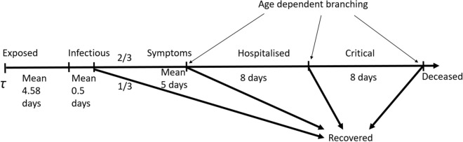
| Intervention | Description |
|---|---|
| No intervention | Business as usual |
| Lockdown | For compliant households, household rates are doubled, no workplace |
| interactions except for 25% leakage (for essential services), community | |
| interactions reduce by 75%. For non-compliant households, workplace | |
| interactions only have a leakage of 25%, community interactions are | |
| unchanged, and household interactions increase by 50% | |
| Case Isolation | Compliant symptomatic individuals stay at home for 7 days, reducing non- |
| household contacts by 75%. Household contacts remain unchanged. | |
| Home Quarantine | Following identification of a symptomatic case in a compliant household, |
| all household members remain at home for 14 days. Household contact | |
| rates double, contacts in the community reduce by 75% | |
| Social distancing of the elderly | All compliant individuals over 65 years of age reduce their community |
| interactions by 75% | |
| Schools and colleges closed | Self explanatory |
| Masks | Reduce community transmission by 20% |