Adversarially Robust Industrial Anomaly Detection Through Diffusion Model

Yuanpu Cao, Lu Lin, Jinghui Chen
The Pennsylvania State University
{ymc5533,lulin,jzc5917}@psu.edu

Abstract

Deep learning-based industrial anomaly detection models have achieved remarkably high accuracy on commonly used benchmark datasets. However, the robustness of those models may not be satisfactory due to the existence of adversarial examples, which pose significant threats to the practical deployment of deep anomaly detectors. Recently, it has been shown that diffusion models can be used to purify the adversarial noises and thus build a robust classifier against adversarial attacks. Unfortunately, we found that naively applying this strategy in anomaly detection (i.e., placing a purifier before an anomaly detector) will suffer from a high anomaly miss rate since the purifying process can easily remove both the anomaly signal and the adversarial perturbations, causing the later anomaly detector failed to detect anomalies. To tackle this issue, we explore the possibility of performing anomaly detection and adversarial purification simultaneously. We propose a simple yet effective adversarially robust anomaly detection method, AdvRAD, that allows the diffusion model to act both as an anomaly detector and adversarial purifier. We also extend our proposed method for certified robustness to $l_{2}$ norm bounded perturbations. Through extensive experiments, we show that our proposed method exhibits outstanding (certified) adversarial robustness while also maintaining equally strong anomaly detection performance on par with the state-of-the-art methods on industrial anomaly detection benchmark datasets.

1 Introduction

Anomaly detection aims at identifying data instances that are inconsistent with the majority of data, which has been widely applied in large-scale industrial manufacturing [6] where efficient automatic anomaly detectors are deployed to spot diverse defects of industrial components varying from detecting scratches and leakages in capsules to finding impaired millimeter-sized components on a complicated circuit board [44]. Recently, deep learning (DL) based anomaly detection methods have achieved remarkable improvement over traditional anomaly detection strategies [33, 28]. DL-based methods take advantage of neural networks to estimate the anomaly score of a data instance which reflects how likely it is an anomaly. One common practice defines anomaly score as the reconstruction error between the original data instance and the recovered one decoded by a symmetric neural network model (e.g., autoencoder) [16, 9]. The insight that the reconstruction error can serve as the anomaly score is that the model trained on normal data usually cannot reproduce anomalous instances [7], thus a high reconstruction error for a data instance indicates a larger probability of it being an anomaly.

Though DL-based anomaly detection methods have achieved remarkably high accuracy on commonly used benchmark datasets [41, 20], the robustness of the detection models is still unsatisfactory due to the existence of adversarial examples [14, 23], which poses significant threats to the practical deployment of deep anomaly detectors. An imperceptible perturbation on the input data could cause a well-trained anomaly detector to return incorrect detection results. Specifically, an anomalous instance, when added with an invisible noise, could cheat the detector to output a low anomaly score; while the normal instance can also be perturbed to make the detector raise a false alarm with a high anomaly score. In fact, such a robustness issue is not unique to a specific model, but a common problem for various state-of-the-art deep anomaly detection models (as will be seen in our later experiments in Section 3).

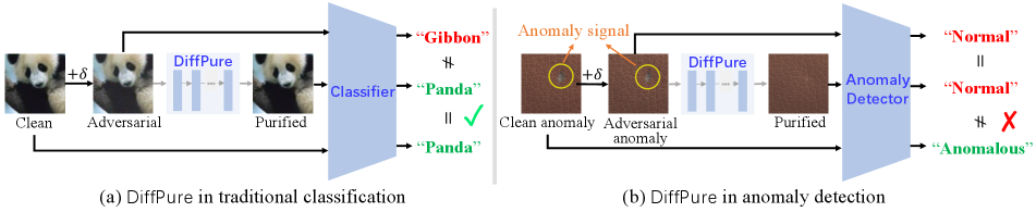
Refer to caption — Figure 1: Left: purification-based adversarial robust model in the traditional classification task. Right: purification-based adversarial robust anomaly detection model. The anomaly signal can also be erased during the purification process leading to a high anomaly miss rate.

Recently, Nie et al. [27] have shown that diffusion models [17, 36] can be used as data purifier to mitigate adversarial noises, and the proposed DiffPure [27] achieves state-of-the-art defense performance. As a powerful class of generative models, diffusion models [17, 26] are capable of generating samples with high quality, beating GANs in image synthesis [13]. Specifically, diffusion models first gradually add random noise and convert the data into standard Gaussian noise, and then learn the generative process to reverse the process and generate samples by denoising one step at a time. The denoising capability of diffusion models makes it possible to use it against imperceptible adversarial perturbations. As shown in Figure 1 (left), DiffPure [27] constructs a robust classifier by leveraging the diffusion model to purify adversarially perturbed images before classification. However, in anomaly detection scenario, naively placing DiffPure [27] before another anomaly detector will largely deteriorate the detection performance as the purifier can also purify the anomaly signals along with the adversarial perturbations. Figure 1 (right) shows a simple case of how DiffPure [27] fails in anomaly detection. We can observe that when receiving an “leather” image with both imperceptible adversarial noise and anomaly signal (i.e., color defects), DiffPure [27] essentially erase the color defects along with the adversarial perturbations, leading to high anomaly miss rate¹¹1We will discuss more experiments in Section 4.2..

The key reason behind the failure of directly applying DiffPure [27] in anomaly detection lies in that the purifying process can easily remove both the anomaly signal and the adversarial perturbations. While in the ideal case, DiffPure should only remove the adversarial perturbation while preserving the anomaly signal for accurate detection later. Given this observation, a natural question arises:

Is it possible to develop a method to simultaneously perform anomaly detection and adversarial purification together?

If the answer is yes, we don’t need to enforce the purifier to distinguish between anomaly signals and adversarial perturbations, which is quite challenging. Based on this motivation, we explore the possibility of making the diffusion model act both as an anomly detector and adversarial purifier simultaneously and propose a novel adversarially robust anomaly detection method, termed AdvRAD.

We summarize our contributions as follows:

•

We build a unified adversarial attack framework for various kinds of anomaly detectors to facilitate the adversarial robustness study in industrial anomaly detection domain, through which we systematically evaluate the adversarial robustness of state-of-the-art deep anomaly detection models.
•

We propose a novel adversarially robust industrial anomaly detection model through the diffusion model, inside which the diffusion model simultaneously performs anomaly detection and adversarial purification. We also extend our method for certified robustness to $l_{2}$ norm perturbations through randomized smoothing which provides additional robustness guarantees.
•

We conduct extensive experiments and show that our method exhibits outstanding (certified) adversarial robustness, while also maintaining equally strong anomaly detection performance on par with the state-of-the-art anomaly detectors on industrial anomaly detection benchmark datasets MVTec AD [6], ViSA [44], and BTAD [25].

2 Related Work

Anomaly Detection Methods Existing anomaly detection methods can be roughly categorized into two kinds: reconstruction-based and feature-based. One commonly used reconstruction-based approach for anomaly detection is to train the autoencoder and use the $l_{p}$ norm distance between input and its reconstruction as the anomaly score [16, 9, 43]. Bergmann et al. [5] replace $l_{p}$ distance with SSIM [38] to have a better measure for perceptual similarity. Another more advanced branch of reconstruction-based models combines autoencoder with GAN, where the generator of the GAN is implemented using autoencoder [18, 22, 1]. These methods additionally incorporate the anomaly score with the similarity between the features of the input and the reconstructed images extracted from the discriminator to boost performance on categories that are difficult to reconstruct accurately. Feature-based methods use pre-trained Resnet and vision transformer [41], or pre-trained neural networks with feature adaptation [20] to extract discriminative features for normal images, and estimate the distribution of these normal features by Flow-based model [15, 32], KNN [30], or Gaussian distribution modeling [21]. These methods calculate the anomaly score using the distance from the features of test images to the established distribution for features of normal images.

Adversarial Attacks and Defenses for Anomaly Detectors To the best of our knowledge, existing attack and defense strategies for anomaly detectors only focus on autoencoder-based models. Goodge et al. [14] consider perturbations to anomalous data that make the model categorize them as the normal class by reducing reconstruction error. For defense, they propose APAE using approximate projection and feature weighting to improve adversarial robustness. Lo et al. [23] extend the similar attack strategy to both normal and anomalous data and propose Principal Latent Space as a defense strategy to perform adversarially robust novelty detection. While they achieve a certain level of robustness, their performances on clean anomaly detection tasks are yet far from satisfactory.

Diffusion Models As a class of powerful generative models, diffusion models have attracted the most recent attention due to their high sample quality and strong mode coverage [34, 17, 26]. Recently, Nie et al. [27] use diffusion models to purify adversarial perturbations for downstream robust classification, and the proposed DiffPure presents empirically strong robustness. In medical diagnostics, Wolleb et al. [39] adopt deterministic DDIM [35] for supervised brain tumor detection. Wyatt et al. [40] solve the same task under an unsupervised scenario using DDPM [17] with specially designed simplex noise for tumorous dataset. Note that these diffusion-based medical anomaly detection methods focusing on pixel-level anomaly are not directly comparable to our image-level anomaly detection. Moreover, none of the previous works have studied to improve the adversarial robustness of anomaly detection through diffusion models. We defer more comparison with the above diffusion model-based anomaly detector in Section 5.3.

3 Building Unified Adversarial Attacks for Anomaly Detectors

To facilitate the adversarial robustness study on various kinds of anomaly detectors, we first build a unified adversarial attack framework in the context of anomaly detection. We consider the adversarial perturbations to be imperceptible, i.e., their existence will not flip the ground truth of the image (normal or anomalous). The general goal of the unified attack is to make detectors return incorrect detection results by reducing anomaly scores for anomalous samples and increasing anomaly scores for normal samples. In particular, we use Projected Gradient Descent (PGD) [24] to build the attack.

PGD Attack on Anomaly Detector Consider a sample ${\mathbf{x}}\in\mathbb{R}^{d}$ from the test dataset with label ${\textnormal{y}}\in\{-1,1\}$ (where “ $-1$ ” denotes the anomalous class and “ $1$ ” indicates the normal class), and a well-trained anomaly detector $A_{{\bm{\theta}}}:\mathbb{R}^{d}\rightarrow\mathbb{R}$ that computes an anomaly score for each data sample. We define the optimization objective of PGD attack on the anomaly detector as: $\operatorname*{arg\,max}_{{\mathbf{x}}}L_{{\bm{\theta}}}({\mathbf{x}},{\textnormal{y}})={\textnormal{y}}A_{{\bm{\theta}}}({\mathbf{x}}),$ where y guides the direction of perturbing ${\mathbf{x}}$ to increase or decrease its anomaly score. Depending on the perturbation constraint, adversarial examples can be generated by $l_{\infty}$ -norm or $l_{2}$ -norm bounded PGD, respectively as:

	$\displaystyle{\mathbf{x}}_{n+1}=P_{{\mathbf{x}},\epsilon}^{l_{\infty}}\left\{{\mathbf{x}}_{n}+\alpha\cdot\text{sgn}(\nabla_{{\mathbf{x}}_{n}}L_{{\bm{\theta}}}({\mathbf{x}}_{n},{\textnormal{y}})\right\}$		(1)
	$\displaystyle{\mathbf{x}}_{n+1}=P_{{\mathbf{x}},\epsilon}^{l_{2}}\left\{{\mathbf{x}}_{n}+\alpha\frac{\nabla_{{\mathbf{x}}_{n}}L_{{\bm{\theta}}}({\mathbf{x}}_{n},{\textnormal{y}})}{\left\\|\nabla_{{\mathbf{x}}_{n}}L_{{\bm{\theta}}}({\mathbf{x}}_{n},{\textnormal{y}})\right\\|}\right\}$		(2)

where $\alpha$ is the step size, $n\in[0,N-1]$ is the current step of in total $N$ iterations, and ${\mathbf{x}}_{0}={\mathbf{x}}$ . $P_{{\mathbf{x}},\epsilon}^{l_{p}}\{\cdot\}$ denotes the projection on ${\mathbf{x}}_{n+1}$ such that $\left\|{\mathbf{x}}_{n+1}-{\mathbf{x}}\right\|_{p}\leq\epsilon$ . The final adversarial example is generated by ${\mathbf{x}}_{adv}={\mathbf{x}}_{N}$ . This attacking strategy encapsulates previous works on adversarial examples for anomaly detectors, where only autoencoder-based models were considered [23, 14]. The anomaly score can be specified as $\displaystyle A_{{\bm{\theta}}}({\mathbf{x}})=\left\|D(E({\mathbf{x}}))-{\mathbf{x}}\right\|$ to accommodate to their scenarios, where $D$ denotes the decoder and $E$ corresponds to the encoder.

Robustness Evaluation on Existing Anomaly Detectors Based on the unified PGD attack, we systematically evaluate the adversarial robustness of the state-of-the-art detectors with various models. Table 1 demonstrates the efficacy of the attack in disclosing the vulnerability of existing anomaly detectors: the AUC scores of these advanced anomaly detectors drop to as low as $0$ under adversarial perturbations with $l_{\infty}$ norm less than $2/255$ on Toothbrush dataset from benchmark MVTec [6]. This suggests that current anomaly detectors suffer from fragile robustness on adversarial data.

Method	OCR-GAN [22]	SPADE [11]	CFlow [15]	FastFlow [41]	CFA [20]
Standard AUC	$96.7$	$88.9$	$85.3$	$94.7$	$100$
Robust AUC	$0$	$0$	$0$	$0$	$0$

Table 1: Standard AUC and robust AUC against

l_{\infty}

-PGD (

\epsilon=2/255

) attacks on Toothbrush dataset from benchmark MVTec AD, obtained by various anomaly detection SOTAs.

4 Adversarially Robust Anomaly Detection

Before we introduce our novel robust anomaly detection method, we first give a brief review of diffusion models [34, 17, 26] and present a naive attempt of applying DiffPure [27] on anomaly detection and analyze its failure case.

Purification-level	$p=5$	$p=25$	$p=50$	$p=100$	$p=200$	$p=300$
Standard AUC	$93.6$	$95.0$	$87.5$	$74.7$	$47.5$	$36.4$
Robust AUC	$32.2(\downarrow 61.4)$	$47.8(\downarrow 47.2)$	$50.6(\downarrow 36.9)$	$34.2(\downarrow 40.5)$	$9.4(\downarrow 38.1)$	$19.7(\downarrow 16.7)$

Table 2: Standard AUC and robust AUC against

l_{\infty}

-PGD

(\epsilon=2/255)

attacks on Toothbrush dataset, obtained by DiffPure [27] + CFA [20] with varying purification-level

p

(diffusion steps, max=1000).

4.1 Preliminaries on Diffusion Models

We follow the formulation of DDPMs given in [17, 26], which defines a $T$ steps diffusion process $q({\mathbf{x}}_{1:T}|{\mathbf{x}}_{0}):=\prod_{t=1}^{T}q({\mathbf{x}}_{t}|{\mathbf{x}}_{t-1})$ parameterized by a variance schedule $\beta_{1},\ldots,\beta_{T}$ as $q({\mathbf{x}}_{t}|{\mathbf{x}}_{t-1}):=\mathcal{N}({\mathbf{x}}_{t};{\mathbf{x}}_{t-1}\sqrt{1-\beta_{t}},\beta_{t}I)$ , which iteratively transforms an unknown data distribution ${q({\mathbf{x}}_{0})}$ to standard Gaussian ${q({\mathbf{x}}_{T})}=\mathcal{N}(0,\mathbf{I})$ . The generative process $p_{\bm{\theta}}({\mathbf{x}}_{0:T}):=p({\mathbf{x}}_{T})\prod_{t=1}^{T}p_{\bm{\theta}}({\mathbf{x}}_{t-1}|{\mathbf{x}}_{t})$ is learned to approximate each $q({\mathbf{x}}_{t-1}|{\mathbf{x}}_{t})$ using neural networks as $p_{\bm{\theta}}({\mathbf{x}}_{t-1}|{\mathbf{x}}_{t}):=\mathcal{N}({\mathbf{x}}_{t-1};\bm{\mu}_{\bm{\theta}}({\mathbf{x}}_{t},t),\bm{\Sigma}_{\bm{\theta}}({\mathbf{x}}_{t},t))$ A noticeable property of the diffusion process is that it allows directly sampling ${\mathbf{x}}_{t}$ at an arbitrary timestep $t$ given ${\mathbf{x}}_{0}$ . Using the notation $\alpha_{t}:=1-\beta_{t}$ and $\overline{\alpha_{t}}:=\prod_{s=1}^{t}\alpha_{s}$ , we have

{\mathbf{x}}_{t}=\sqrt{\overline{\alpha}_{t}}{\mathbf{x}}_{0}+\sqrt{1-\overline{\alpha}_{t}}\bm{\epsilon},\quad\bm{\epsilon}\in\mathcal{N}(0,\mathbf{I})

(3)

For training the diffusion model, Ho et al. [17] propose a simplified objective without learning signals for $\bm{\Sigma}_{\bm{\theta}}({\mathbf{x}}_{t},t)$ : $L_{\text{simple}}=\mathbb{E}_{t,{\mathbf{x}}_{0},\bm{\epsilon}}[\|\bm{\epsilon}-\bm{\epsilon}_{{\bm{\theta}}}({\mathbf{x}}_{t},t)\|]$ In this paper, we follow Nichol and Dhariwal [26] and train the diffusion model using a hybrid loss for better sample quality with fewer generation steps. More details can be found in Appendix A.

4.2 Naive Attempt: Applying DiffPure on Anomaly Detection

DiffPure [27] uses the diffusion model to purify adversarially perturbed images before classification and present strong empirical robustness. A naive idea would be applying DiffPure in anomaly detection for better robustness. However, as mentioned previously, naively placing a purifier before another anomaly detector will largely deteriorate the detection performance as the purifier can also purify the anomaly signals along with the adversarial perturbations. For this strategy to work, DiffPure should only remove the adversarial perturbation while preserving the anomaly signal for anomaly detection later. Unfortunately, this is extremely difficult to achieve. To verify this, we directly apply DiffPure [27] upon CFA [20], one of the SOTA anomaly detectors, with different purification levels (i.e., diffusion steps in DiffPure [27]) and present the results in Table 2. We can observe that, with a lower purification level (e.g., 5, 25 diffusion steps), this method maintains high standard AUC while the robust AUC is far from satisfactory, suggesting that it is unable to fully remove the adversarial perturbations; when increasing the purification level, standard AUC will rapidly decrease, suggesting that the anomaly signal was also removed. This observation motivates us to build adversarially robust anomaly detectors that can simultaneously perform anomaly detection and adversarial purification.

4.3 Merging Anomaly Detection and Adversarial Purification through Diffusion Model

Observing the failure case of naively applying DiffPure on anomaly detection, it is natural to ask whether we can simultaneously perform anomaly detection and adversarial purification together. If so, we can avoid enforcing the purifier to distinguish between anomaly signals and adversarial perturbations. Surprisingly, we found a simple yet effective strategy to merge anomaly detection and adversarial purification tasks into one single robust reconstruction procedure through the diffusion model. We named this adversarially robust anomaly detection method AdvRAD.

Robust Reconstruction Robust reconstruction in AdvRAD is the key to merging anomaly detection and adversarial purification tasks together. It relies on the fact that the diffusion model itself can be used as a reconstruction model and the reconstruction error can be used as a natural anomaly score. Specifically, the diffusion model training procedure is essentially predicting noise added in the diffusion process and then denoising. Instead of using the trained diffusion model to generate new samples through multiple denoising steps from a noise, one can also start from an original image, gradually add noise and then denoise to reconstruct the original image. Since the diffusion model is trained on the normal data samples, such reconstruction error can serve as a natural indicator of the anomaly score. In Figure 2, we show an example of robust reconstruction using diffusion models. As can be seen from Figure 2, for normal data, the reconstruction is nearly identical to the input. For anomaly data, the diffusion model (after adding noise and denoising) could “repair” the anomaly regions, thus obtaining high reconstruction error, which could be easily detected as anomalies. Now let’s consider adversarial robustness in anomaly detection. From Section 4.2, we already know that the adversarial noise will be removed together with the anomaly signal by the diffusion model. Therefore, after robust reconstruction, the adversarially perturbed anomaly sample could still be recovered to normal case and thus obtain a high reconstruction error as shown in Figure 2. In this way, AdvRAD no longer needs to distinguish between adversarial noise and anomaly signal and thus only needs to remove both simultaneously. We summarize the robust construction steps in Algorithm 2 in Appendix B.

To obtain the best performances of AdvRAD, there are still several things to notice: 1) The diffusion steps $k$ in robust reconstruction should be chosen such that the amount of Gaussian noise is dominating the adversarial perturbations and anomaly signals while the high-level features of the input data are still preserved for reconstruction. 2) One major problem with the traditional diffusion denoising algorithm (see Algorithm 2 in Appendix B) is that the iterative denoising procedure is time-consuming, making it unacceptable for real-time anomaly detection in critical situations [37]. Moreover, extra reconstruction error can also be introduced due to the multiple sampling steps. To overcome these challenges, we investigate the arbitrary-shot denoising process allowing fewer denoising steps, with the details shown in Appendix B.2. Based on our results (see Appendix D.5) we observe that one-shot denoising (Algorithm 1) is sufficient to produce an accurate reconstruction result with $\mathcal{O}(1)$ inference-time efficiency. Such a one-shot idea has also been adopted in Carlini et al. [8] for robust image classification. By default, we use one-shot robust reconstruction for all experiments in Section 5.

Algorithm 1 One-shot Robust Reconstruction in AdvRAD

1: Input: Test images:

{\mathbf{x}}

, diffusion steps:

k(k\leq T)

2: Output: Reconstructions of

{\mathbf{x}}

\tilde{{\mathbf{x}}}

\bm{\epsilon}\sim\mathcal{N}(0,\mathbf{I})

{\mathbf{x}}_{k}=\sqrt{\overline{\alpha}_{k}}{\mathbf{x}}_{0}+\sqrt{1-\overline{\alpha}_{k}}\bm{\epsilon}

// one-shot denoising process:

\tilde{{\mathbf{x}}}=\frac{1}{\sqrt{\overline{\alpha}_{k}}}({{\mathbf{x}}}_{k}-\sqrt{1-\overline{\alpha}_{k}}\bm{\epsilon}_{{\bm{\theta}}}({\mathbf{x}}_{k},k))

Anomaly Score Calculation: To calculate the final anomaly score in a robust and stable manner, we first calculate the Multiscale Reconstruction Error Map (denoted as $\text{Err}_{\text{ms}}$ ), which considers both pixel-wise and patch-wise reconstruction errors. Specifically, for each scale $l$ in $L=\{1,\frac{1}{2},\frac{1}{4},\frac{1}{8}\}$ , we first calculate the error map ${\text{Err}({\mathbf{x}},\tilde{{\mathbf{x}}})}_{l}$ between the downsampled input ${{\mathbf{x}}}^{l}$ and the downsampled reconstruction ${\tilde{{\mathbf{x}}}}^{l}$ with $\frac{1}{C}\sum_{c=1}^{C}{({{\mathbf{x}}}^{l}-{\tilde{{\mathbf{x}}}}^{l})}_{[c,:,:]}^{2}$ where the square operator is abused here for element-wise square operation, then unsampled to the original resolution. The final $\text{Err}_{\text{ms}}$ is obtained by averaging each scale’s error map and applying a mean filter for better stability similar to Zavrtanik et al. [42]: ${\text{Err}_{\text{ms}}({\mathbf{x}},\tilde{{\mathbf{x}}})}=(\frac{1}{N_{L}}\sum_{l\in L}{\text{Err}({\mathbf{x}},\tilde{{\mathbf{x}}})}_{l})\ast f_{s\times s}$ where $f_{s\times s}$ is the mean filter of size ${s\times s}$ , $\ast$ is the convolution operation. Similar to Pirnay and Chai [29], we take the pixel-wise maximum of the absolute deviation of the $\text{Err}_{\text{ms}}({\mathbf{x}},\tilde{{\mathbf{x}}})$ on normal training data as the scalar anomaly score. Due to space limits, we leave the complete anomaly score calculation algorithm in Appendix B.3.

5 Experiments

We compare our proposed AdvRAD with state-of-the-art anomaly detectors on both clean input and adversarially perturbed input. AdvRAD shows a stronger robustness performance compared with SOTAs even combined with model-agnostic defenses (i.e., DiffPure [27] and Adversarial Training [24]) and domain-specific defense-enabled anomaly detector baselines, and also maintains robustness even under stronger adaptive attacks. Finally, we further extend AdvRAD for certified robustness to $l_{2}$ norm perturbations.

5.1 Experimental Settings

Dataset and Model Implementation: We perform experiments on three industrial anomaly detection benchmark datasets MVTec AD [6], ViSA [44] and BTAD [25] datasets. MVTec AD comprises 15 different texture (e.g., leather, wood) and object (e.g., toothbrush, transistor) categories which showcase more than $70$ types of anomalies from the real world. ViSA covers 12 objects with challenging scenarios including complex structures, multiple instances and object pose/location variations. BTAD contains $3$ industrial products showcasing body and surface anomalies. We resize all images to 256 $\times$ 256 resolution in our experiments. We implement the diffusion model based on Nichol and Dhariwal [26] using U-Net backbone [31]. We set the total iteration step as $T=1000$ for all experiments. During the inference stage, we choose the diffusion step $k=100$ in our experiments (see Appendix D.4 for sensitivity test). More hyperparameters are described in Appendix C.1.

Adversarial Attacks: We adopt commonly used PGD attack [24] to compare with the state-of-the-art anomaly detection models and defense-enabled anomaly detectors. Additionally, we also consider the BPDA, EOT attack [3], and AutoAttack [12] for better robustness evaluations on defense-enabled anomaly detectors and ours. We set the attack strength $\epsilon=2/255$ for $l_{\infty}$ -norm attacks and $\epsilon=0.2$ for $l_{2}$ -norm attacks to ensure imperceptible attack perturbations.

Evaluation Metric: We use the widely-adopted AUC (area under the receiver operating characteristic curve) to evaluate anomaly detection performance. Specifically, we consider standard AUC and robust AUC. The standard AUC evaluates the performance on the clean test data, while the robust AUC evaluates the performance on adversarially perturbed data.

5.2 Comparison with the State-of-the-art Anomaly Detectors

We compare our method AdvRAD with five state-of-the-art methods for image anomaly detection: SPADE [11], OCR-GAN [22], CFlow [15], FastFlow [41], and CFA [20], against the $l_{\infty}$ -PGD and $l_{2}$ -PGD attacks. Table 3, 4 and 5 present the robustness performance against $l_{\infty}$ -PGD attacks ( $\epsilon=2/255$ ) on MVTec AD, ViSA and BTAD, respectively. We observe that our method largely outperforms previous methods regarding robust AUC against $l_{\infty}$ -PGD attacks ( $\epsilon=2/255$ ). Specifically, our method improves robust AUC on all $15$ categories of MVTec AD and obtains the average robust AUC of $81.1\%$ with the improvement of at least $78.8\%$ . In ViSA and BTAD, our method improves the avg robust AUC by $80.6\%$ and $72.6\%$ , respectively. See Appendix D.1 for similar results against $l_{2}$ -PGD attacks ( $\epsilon=0.2$ ). In the meantime, we can observe that in terms of anomaly detection performance on clean data, the average standard AUC obtained by our method is on par with the state-of-the-art methods in MVTec AD and BTAD datasets, while beating all baselines in ViSA. These results clearly demonstrate the effectiveness of our proposed method in defending against $l_{\infty}$ -PGD and $l_{2}$ -PGD attacks, while also maintaining strong anomaly detection performance on benchmark datasets.

Category	OCR-GAN	SPADE	CFlow	FastFlow	CFA	AdvRAD
Carpet	$0^{(76.6)}$	$0^{(92.8)}$	$0^{(98.6)}$	$0^{(\mathbf{99.7})}$	$0^{(99.4)}$	$\mathbf{70.5}^{(73.8)}$
Grid	$0^{(97)}$	$0^{(47.3)}$	$0^{(96.6)}$	$0^{(\mathbf{100})}$	$0^{(99.6)}$	$\mathbf{99.6}^{(\mathbf{100})}$
Leather	$0^{(90.7)}$	$0^{(95.4)}$	$0^{(\mathbf{100})}$	$6.6^{(\mathbf{100})}$	$2.0^{(\mathbf{100})}$	$\mathbf{97.8}^{(\mathbf{100})}$
Tile	$0^{(95.6)}$	$0^{(96.5)}$	$0^{(99.6)}$	$1.3^{(\mathbf{100})}$	$0.1^{(99.3)}$	$\mathbf{93.9}^{(95.4)}$
Wood	$0^{(95.4)}$	$0^{(95.8)}$	$0^{(99.7)}$	$0^{(\mathbf{99.9})}$	$0^{(99.7)}$	$\mathbf{95.2}^{(98.3)}$
Bottle	$0^{(97.7)}$	$0^{(97.2)}$	$0^{(\mathbf{100})}$	$0^{(\mathbf{100})}$	$0.1^{(\mathbf{100})}$	$\mathbf{96.9}^{(99.6)}$
Cable	$0^{(71.5)}$	$0^{84.8)}$	$0^{(98.7)}$	$0^{(67.4)}$	$0.8^{(\mathbf{99.8})}$	$\mathbf{38.9}^{(79.2)}$
Capsule	$0^{(80.4)}$	$0^{(89.7)}$	$0^{(93.7)}$	$8.9^{(\mathbf{99.2})}$	$0^{(97)}$	$\mathbf{53.5}^{(90.5)}$
Hazelnut	$0^{(97.7)}$	$0^{(88.1)}$	$0^{(99.9)}$	$0^{(99.5)}$	$0.1^{(\mathbf{100})}$	$\mathbf{91.5}^{(97.3)}$
Metal Nut	$0^{(82.6)}$	$0^{(71)}$	$0^{(\mathbf{100})}$	$0^{(98.2)}$	$0^{(\mathbf{100})}$	$\mathbf{85.9}^{(91.0)}$
Pill	$0^{(80.8)}$	$0^{(80.1)}$	$0^{(93.2)}$	$0^{(97.8)}$	$0^{(\mathbf{98})}$	$\mathbf{39.0}^{(94.4)}$
Screw	$0^{(\mathbf{99.4})}$	$0^{(66.7)}$	$0^{(79)}$	$6.6^{(91.1)}$	$0^{(95.5)}$	$\mathbf{87.6}^{(99.3)}$
Toothbrush	$0^{(96.7)}$	$0^{(88.9)}$	$0^{(85.3)}$	$0^{(94.7)}$	$0^{(\mathbf{100})}$	$\mathbf{95.8}^{(\mathbf{100})}$
Transistor	$0^{(75)}$	$0^{(90.3)}$	$0^{(98.3)}$	$0^{(99.4)}$	$0^{(\mathbf{100)}}$	$\mathbf{74.5}^{(90.6)}$
Zipper	$0^{(80.4)}$	$0^{(96.6)}$	$0^{(97.5)}$	$17.5^{(99.6)}$	$0^{(99.7)}$	$\mathbf{96.2}^{(\mathbf{99.7})}$
Average	$0^{(87.8)}$	$0^{(85.4)}$	$0^{(96.0)}$	$2.3^{(98.5)}$	$0.2^{(\mathbf{99.2})}$	$\mathbf{81.1}^{(93.9)}$

Table 3: Robust AUC

{}^{\text{(Standard AUC)}}

against

l_{\infty}

-PGD attacks on MVTec AD, obtained by SOTAs and ours.

Category	SPADE	CFlow	FastFlow	CFA	AdvRAD
PCB1	$0^{(88.9)}$	$0^{(95.0)}$	$0^{(88.8)}$	$1.6^{(92.7)}$	$\mathbf{87.6}^{(\mathbf{95.9})}$
PCB2	$0^{91.8)}$	$0^{(87.3)}$	$0.1^{(88.7)}$	$1.5^{(93.7)}$	$\mathbf{94.6}^{(\mathbf{99.4})}$
PCB3	$0^{(81.1)}$	$0^{(82.1)}$	$0^{(87.3)}$	$2.4^{(94.3)}$	$\mathbf{96.9}^{(\mathbf{99.4})}$
PCB4	$0^{(\mathbf{95.7})}$	$0^{(97.8)}$	$0^{(96.5)}$	$0^{(\mathbf{99.6})}$	$\mathbf{97.6}^{(99.3)}$
Capsules	$0^{(63.9)}$	$0^{(58.3)}$	$0^{(74.3)}$	$0^{(64.7)}$	$\mathbf{73.1}^{(\mathbf{88.4})}$
Candle	$0^{(89.0)}$	$0^{(95.6)}$	$0^{(\mathbf{95.8})}$	$0^{(91.6)}$	$\mathbf{63.3}^{(92.2)}$
Macaroni1	$0^{(80.7)}$	$0^{(84.3)}$	$0^{(89.1)}$	$0^{(87.5)}$	$\mathbf{83.5}^{(\mathbf{99.0})}$
Macaroni2	$0^{(60.5)}$	$0^{(72.7)}$	$0^{(72.4)}$	$0^{(76.5)}$	$\mathbf{70.6}^{(\mathbf{93.0})}$
Cashew	$0^{(93.2)}$	$0^{(93.9)}$	$0^{(91.4)}$	$0.1^{(\mathbf{94.0})}$	$\mathbf{72.4}^{(\mathbf{97.3})}$
Chewing gum	$0^{(95.3)}$	$0^{(98.0)}$	$0.4^{(\mathbf{99.1})}$	$2.2^{(\mathbf{99.4})}$	$\mathbf{80.1}^{(\mathbf{99.4})}$
Fryum	$0^{(91.3)}$	$0^{(86.2)}$	$2.0^{(\mathbf{93.8})}$	$0.6^{(92.6)}$	$\mathbf{77.2}^{(93.7)}$
Pipe fryum	$0^{(74.0)}$	$0^{(97.6)}$	$0^{(96.5)}$	$0^{(96.1)}$	$\mathbf{79.1}^{(\mathbf{98.3})}$
Average	$0^{(83.8)}$	$0^{(87.4)}$	$0.2^{(89.5)}$	$0.7^{(90.2)}$	$\mathbf{81.3}^{(\mathbf{96.3})}$

Table 4: Robust AUC

{}^{\text{(Standard AUC)}}

against

l_{\infty}

-PGD attacks on ViSA, obtained by SOTAs and ours.

Category	SPADE	CFlow	FastFlow	CFA	AdvRAD
01	$0^{(94.5)}$	$2.0^{(96.9)}$	$5.6^{(99.4)}$	$43.2^{(\mathbf{100})}$	$\mathbf{100}^{(\mathbf{100})}$
02	$0^{(77.0)}$	$0^{(84.2)}$	$22.4^{(\mathbf{84.5})}$	$2.2^{(83.2)}$	$\mathbf{63.9}^{(79.9)}$
03	$0^{(\mathbf{100})}$	$1.2^{(99.9)}$	$7.0^{(94.5)}$	$0.1^{(99.6)}$	$\mathbf{99.5}^{(\mathbf{100})}$
Average	$0^{(90.5)}$	$1.1^{(93.7)}$	$11.7^{(92.8)}$	$15.2^{(\mathbf{94.3})}$	$\mathbf{87.8}^{(93.2)}$

Table 5: Robust AUC

{}^{\text{(Standard AUC)}}

against

l_{\infty}

-PGD attacks on BTAD dataset, obtained by SOTAs and ours.

5.3 Comparisons with other Diffusion model based Anomaly Detectors

Current diffusion model-based anomaly detection methods primarily focus on medical images [40, 39]. Wolleb et al. [39] adopt deterministic DDIM [35] for supervised pixel-level tumor localization, where the ground truth of the image is required, which is fundamentally different from our unsupervised image-level anomaly detection. Wyatt et al. [40] proposes AnoDDPM to solve the same task under an unsupervised scenario using DDPM [17] with simplex noise. Note that AnoDDPM [40] is also a pixel-level anomaly localization method which is not directly comparable to our image-level anomaly detection. To make the comparison with AnoDDPM [40], we use two image-level anomaly score calculation methods to convert it to an image-level anomaly detector: (1) the maximum pixel anomaly score (i.e., the maximum square error between the reconstruction and the initial image), and (2) our proposed anomaly score calculation as presented in Appendix B.3.

We summarize the (standard AUC, robust AUC) of AnoDDPM [40] and our proposed AdvRAD against $l_{\infty}$ -PGD attacks on MVTec AD [6] in Table 6 where AnoDDPM^∗ refers to AnoDDPM with our proposed anomaly score calculation. We can clearly observe that our proposed AdvRAD outperforms both AnoDDPM [40] and AnoDDPM with the one-shot reconstruction in terms of standard AUC on clean data and robust AUC on perturbed data, which demonstrates that simplex noise cannot generalize well to industrial anomaly detection and deteriorate the adversarial robustness of the diffusion model in anomaly detection. Note that we only evaluate the robustness of AnoDDPM with our one-shot reconstruction for a fair comparison since AdvRAD performs one-shot reconstruction. Moreover, we found that the one-shot technique also improves the performance of AnoDDPM [40] on clean data. Although Wolleb et al. [39], Wyatt et al. [40] have proposed using diffusion models for anomaly detection, and AnoDDPM [40] adopt a similar algorithm framework with our proposed method, none of them have provided the understanding of diffusion model in anomaly detection from a robustness perspective. In addition, the experimental results evidently show that our proposed method outperforms AnoDDPM in terms of accuracy, efficiency, and adversarial robustness in industrial anomaly detection.

Category	AnoDDPM	AnoDDPM (one-shot)	AnoDDPM^∗ (one-shot)	AdvRAD
Carpet	$(72.4,-)$	${(73.7,20.2)}$	${(69.9,9.7)}$	$(\mathbf{73.8},\mathbf{70.5})$
Grid	$(99.2,-)$	${(99.9,81.6)}$	${(\mathbf{100},41.4)}$	${(\mathbf{100},\mathbf{99.6})}$
Leather	$(81.8,-)$	${(91.9,56.4)}$	${(93.4,32.5)}$	${(\mathbf{100},\mathbf{97.8})}$
Tile	$(85.8,-)$	${(80.6,38.7)}$	${(92.0,16.2)}$	${(\mathbf{95.4},\mathbf{93.9})}$
Wood	$(90.2,-)$	${(94.8,42.1)}$	${(94.1,12.6)}$	${(\mathbf{98.3},\mathbf{95.2})}$
Bottle	$(94.8,-)$	${(95.6,81.2)}$	${(97.1,77.8)}$	${(\mathbf{99.6},\mathbf{96.9})}$
Cable	$(57.3,-)$	${(80.5,1.4)}$	${(\mathbf{82.4},0.1)}$	${(79.2,\mathbf{38.9})}$
Capsule	$(74.3,-)$	${(74.5,47.8)}$	${(67.3,33.9)}$	${(\mathbf{90.5},\mathbf{53.5})}$
Hazelnut	$(83.3,-)$	${(85.5,13.9)}$	${(74.5,4.4)}$	${(\mathbf{97.3},\mathbf{91.5})}$
Metal Nut	$(75.6,-)$	${(85.2,9.6)}$	${(88.5,3.7)}$	${(\mathbf{91.0},\mathbf{85.9})}$
Pill	$(59.4,-)$	${(60.7,\mathbf{49.8})}$	${(71.0,31.7)}$	${(\mathbf{94.4},39.0)}$
Screw	$(74.7,-)$	${(69.1,0.3)}$	${(59.6,0.9)}$	${(\mathbf{99.3},\mathbf{87.6})}$
Toothbrush	$(99.7,-)$	${(99.4,14.7)}$	${(\mathbf{100},16.9)}$	${(\mathbf{100},\mathbf{95.8})}$
Transistor	$(68.5,-)$	${(64.6,0.5)}$	${(70.9,0.0)}$	${(\mathbf{90.6},\mathbf{74.5})}$
Zipper	$(89.0,-)$	${(91.9,72.2)}$	${(98.9,64.1)}$	${(\mathbf{99.7},\mathbf{96.2})}$
Average	$(80.4,-)$	${(83.2,35.33)}$	${(84.0,23.1)}$	${(\mathbf{93.9},\mathbf{81.1})}$

Table 6: (Standard AUC, Robust AUC) against

l_{\infty}

-PGD attacks (

\epsilon=2/255

) on MVTec AD, obtained by AnoDDPM and ours.

5.4 Comparison with Model-agnostic Defending Strategies

Category	DiffPure + CFA						AdvRAD
Category	$p=5$	$p=25$	$p=50$	$p=100$	$p=200$	$p=300$	AdvRAD
Carpet	$9.6^{(\mathbf{96.4})}$	$36.2^{(93.4)}$	$51.8^{(91.9)}$	$44.2^{(74.3)}$	$28.6^{(45.0)}$	$30.0^{(42.5)}$	$\mathbf{70.5}^{(73.8)}$
Grid	$24.6^{(94.0)}$	$27.0^{(92.9)}$	$33.3^{(85.0)}$	$32.7^{(73.4)}$	$21.9^{(58.2)}$	$19.8^{(48.7)}$	$\mathbf{99.6}^{(\mathbf{100})}$
Leather	$47.4^{(98.3)}$	$63.8^{(90.8)}$	$61.6^{(86.7)}$	$72.5^{(87.6)}$	$57.1^{(65.9)}$	$47.2^{(62.2)}$	$\mathbf{97.8}^{(\mathbf{100})}$
Tile	$27.4^{(\mathbf{99.4})}$	$49.1^{(99.4)}$	$62.5^{(97.7)}$	$70.8^{(92.7)}$	$67.4^{(86.7)}$	$62.5^{(77.0)}$	$\mathbf{93.9}^{(95.4)}$
Wood	$53.7^{(\mathbf{98.9})}$	$67.2^{(98.5)}$	$66.8^{(92.5)}$	$58.0^{(77.2)}$	$48.3^{(61.1)}$	$42.9^{(53.1)}$	$\mathbf{95.2}^{(98.3)}$
Bottle	$93.0^{(\mathbf{99.8})}$	$93.9^{(99.2)}$	$95.2^{(98.9)}$	$95.6^{(98.5)}$	$91.0^{(96.1)}$	$90.7^{(94.4)}$	$\mathbf{96.9}^{(99.6)}$
Cable	$3.7^{(\mathbf{89.8})}$	$25.7^{(86.4)}$	$38.7^{(83.3)}$	$51.6^{(80.9)}$	$60.3^{(79.1)}$	$\mathbf{63.4}^{(74.6)}$	$38.9^{(79.2)}$
Capsule	$3.7^{(\mathbf{80.9})}$	$27.0^{(70.4)}$	$28.0^{(60.2)}$	$31.4^{(55.1)}$	$39.2^{(57.6)}$	$42.0^{(54.4)}$	$\mathbf{53.5}^{(\mathbf{90.5})}$
Hazelnut	$9.8^{(\mathbf{99.8})}$	$50.7^{(97.3)}$	$58.4^{(94.9)}$	$68.7^{(91.8)}$	$77.4^{(85.4)}$	$73.0^{(76.2)}$	$\mathbf{91.5}^{(97.3)}$
Metal Nut	$0.1^{(\mathbf{98.3})}$	$22.0^{(90.3)}$	$34.4^{(82.1)}$	$37.2^{(69.7)}$	$40.2^{(61.0)}$	$46.6^{(59.1)}$	$\mathbf{85.9}^{(91.0)}$
Pill	$0.1^{(\mathbf{94.7})}$	$15.2^{(89.4)}$	$27.2^{(83.3)}$	$38.2^{(73.4)}$	$44.1^{(63.8)}$	$\mathbf{44.4}^{(60.5)}$	$39.0^{(94.4)}$
Screw	$0^{(64.2)}$	$2.8^{(55.5)}$	$8.1^{(51.9)}$	$15.7^{(53.7)}$	$24.3^{(49.0)}$	$24.4^{(43.3)}$	$\mathbf{87.6}^{(99.3)}$
Toothbrush	$32.2^{(93.6)}$	$47.8^{(95.0)}$	$50.6^{(87.5)}$	$34.2^{(74.7)}$	$9.4^{(47.5)}$	$19.7^{(36.4)}$	$\mathbf{95.8}^{(\mathbf{100})}$
Transistor	$12.2^{(\mathbf{94.6})}$	$48.6^{(92.8)}$	$67.8^{(92.8)}$	$75.6^{(90.4)}$	$\mathbf{77.4}^{(87.1)}$	$75.8^{(85.8)}$	$74.5^{(90.6)}$
Zipper	$22.7^{(95.6)}$	$58.8^{(92.0)}$	$69.8^{(91.5)}$	$71.2^{(87.3)}$	$63.6^{(80.8)}$	$61.2^{(77.5)}$	$\mathbf{96.2}^{(\mathbf{99.7})}$
Average	$22.7^{(93.2)}$	$42.4^{(89.6)}$	$50.3^{(85.3)}$	$53.2^{(78.7)}$	$50.0^{(68.3)}$	$49.6^{(63.0)}$	$\mathbf{81.1}^{(\mathbf{93.9})}$
$01$	$83.1^{(100)}$	$89.8^{(99.9)}$	$89.7^{(99.2)}$	$89.5^{(95.5)}$	$89.2^{(94.6)}$	$83.5^{(95.4)}$	$\mathbf{100}^{(\mathbf{100})}$
$02$	$26.0^{(\mathbf{80.1})}$	$40.6^{(77.1)}$	$41.7^{(75.5)}$	$46.3^{(73.6)}$	$54.0^{(76.3)}$	$53.5^{(71.1)}$	$\mathbf{63.9}^{(79.9)}$
$03$	$16.2^{(99.5)}$	$75.2^{(99.3)}$	$87.0^{(98.8)}$	$88.1^{(\mathbf{97.6})}$	$75.5^{(88.2)}$	$47.7^{(66.6)}$	$\mathbf{99.5}^{(\mathbf{100})}$
Average	$41.8^{(\mathbf{93.2})}$	$68.5^{(92.1)}$	$72.8^{(91.2)}$	$74.6^{(89.8)}$	$72.9^{(86.4)}$	$61.6^{(77.7)}$	$\mathbf{87.8}^{(\mathbf{93.2})}$

Table 7: Robust AUC

{}^{\text{(Standard AUC)}}

against

l_{\infty}

-PGD attacks on MVTec AD (first sixteen rows) and BTAD (last four rows) , obtained by DiffPure + CFA and ours.

Method	BTAD
Method	$01$	$02$	$03$	Average
AT + FastFlow	$0^{(99.4)}$	$0^{(\mathbf{85.9})}$	$14.7^{(90.5)}$	$4.9^{(91.9)}$
AT + CFA	$63.4^{(98.9)}$	$10.2^{(66.8)}$	$5.7^{(99.6)}$	$26.4^{(88.4)}$
AdvRAD	$\mathbf{100}^{(\mathbf{100})}$	$\mathbf{63.9}^{(79.9)}$	$\mathbf{99.5}^{(\mathbf{100})}$	$\mathbf{87.8}^{(\mathbf{93.2})}$

Table 8: Robust AUC

{}^{\text{(Standard AUC)}}

against

l_{\infty}

-PGD attacks on BTAD, obtained by AT + FastFlow, AT + CFA and ours.

In this section, we apply two model-agnostic adversarial defenses on SOTA anomaly detectors to build defending baselines: DiffPure [27] and Adversarial Training [24], which are widely used in supervised classification.

Comparison with applying DiffPure on SOTA anomaly detector We compare our method with DiffPure [27] + CFA [20] which is the best-performing anomaly detector on clean data as presented in Table 3 and 5. We test varying purification levels $p$ (diffusion steps in DiffPure [27] ) to fully verify the effectiveness of the purification strategy. Table 7 summarizes the standard AUC and robust AUC against $l_{\infty}$ -PGD attacks of this baseline and our method on MVTec AD and BTAD, which shows that our method enjoys a significant advantage in terms of average standard AUC and robust AUC. The results suggest that it is infeasible to tune a purification level that makes DiffPure only remove adversarial noise while preserving the anomaly signal for robust and accurate detection. See more results on ViSA in Appendix D.2.

Comparison with applying Adversarial Training on SOTA anomaly detector We additionally compare our method with using Adversarial Training (AT) [24] on SOTA anomaly detectors. Note that AT also has flaws in protecting anomaly detectors since anomaly detection models are usually trained only on normal data [7], which means we can only perform AT on the normal class of data without protection on the robustness of any anomalies data, thus still posing significant threats to the model. The results in Table 8 show that our method outperforms the SOTA anomaly detectors with Adversarial Training on both clean data and adversarial data.

5.5 Comparison with defense-enabled Anomaly Detectors

Except for model-agnostic defending strategies, there are also domain-specific defenses explicitly designed for anomaly detection. In this section, we compare our method with APAE [14] and PLS [23], two defense-enabled anomaly detection methods. We also compare our method with Robust Autoencoder (RAE) [43], which is proposed to handle noise and outlier data points. Since APAE has an optimization loop in their defense process which is hard to backpropagate, we further adopt the BPDA attack [3] designed specifically for obfuscated gradient defenses to evaluate both our method and APAE for a fair comparison. From Table 9 we can observe that AdvRAD largely outperforms them under all attacks.

Method	Standard AUC (Avg)	Robust AUC (Avg)
Method	Standard AUC (Avg)	$l_{\infty}$ -PGD	$l_{2}$ -PGD	$l_{\infty}$ -BPDA	$l_{2}$ -BPDA
RAE	$57.1$	$16.8$	$49.8$	-	-
PLS	$46.4$	$16.0$	$40.8$	-	-
APAE	$64.7$	$29.9$	$61.2$	$30$	$61.2$
AdvRAD	$\mathbf{93.9}$	$\mathbf{81.1}$	$\mathbf{88.8}$	$\mathbf{88.3}$	$\mathbf{89.6}$

Table 9: Avg Robust AUC

{}^{\text{(Avg Standard AUC)}}

against PGD/BPDA attacks on MVTec AD, obtained by RAE, PLS , APAE and ours.

5.6 Defending against Stronger Adaptive Attacks

So far we have shown that AdvRAD is indeed robust to PGD and BPDA attacks. To verify its robustness in more challenging settings, we test AdvRAD against adaptive attacks where the attacker is assumed to already know about our diffusion-based anomaly detection and design attacks against our defense adaptively. Since the diffusion process in our method introduces extra stochasticity, which plays an important role in defending against adversarial perturbations, we consider applying EOT to PGD, which is designed for circumventing randomized defenses. In particular, EOT calculates the expected gradients over the randomization as a proxy for the true gradients of the inference model using Monte Carlo estimation [4, 3, 19]. Table 10 shows the robust AUC against EOT-PGD attacks on ViSA dataset. We observe that the adversarial robustness is not affected too much by EOT. Specifically, the average robust AUC slightly drops $7.4\%$ and $0.8\%$ compared against standard $l_{\infty}$ -PGD and $l_{2}$ -PGD attacks, respectively. These results suggest that our method has empirically strong robustness against adaptive attacks with EOT. Since other baselines use deterministic inference models, it is unnecessary to apply EOT to evaluate their adversarial robustness. Additionally, We incorporate another strong adaptive attack, AutoAttack [12] which ensembles multiple white-box and black-box attacks such as APGD attacks [12] and Square attacks [2]. We summarize the robustness performance of method against AutoAttack in Table 14 which we defer to Appendix D.3. The robust AUC scores of AdvRAD against AutoAttack are still largely higher than other SOTAs against relatively weaker PGD attacks.

Category	$l_{\infty}$ -PGD	$l_{\infty}$ -EOT-PGD	$l_{2}$ -PGD	$l_{2}$ -EOT-PGD
PCB1	$87.6$	$81.3$	$91.0$	$90.5$
PCB2	$94.6$	$91.3$	$96.2$	$97.2$
PCB3	$96.9$	$92.9$	$98.5$	$98.0$
PCB4	$97.6$	$96.0$	$98.2$	$97.9$
Capsules	$73.1$	$68.7$	$77.9$	$76.7$
Candle	$63.3$	$46.2$	$74.2$	$69.8$
Macaroni1	$83.5$	$77.9$	$89.5$	$90.5$
Macaroni2	$70.6$	$65.6$	$78.1$	$77.1$
Cashew	$72.4$	$51.2$	$86.1$	$86.0$
Chewing gum	$80.1$	$67.7$	$92.8$	$91.1$
Fryum	$77.2$	$72.5$	$85.3$	$84.8$
Pipe fryum	$79.1$	$75.8$	$88.8$	$88.5$
Average	$81.3$	$73.9(\downarrow$ 7.4 $)$	$88.1$	$87.3(\downarrow$ 0.8 $)$

Table 10: Robust AUC against

l_{\infty}

-PGD,

l_{\infty}

-EOT-PGD, and

l_{2}

-PGD,

l_{2}

-EOT-PGD attacks (EOT=

20

) on ViSA dataset.

5.7 Extension: Certified Adversarial Robustness

Noise	Certified AUC at $l_{2}$ radius $\epsilon$
Noise	0	0.05	0.1	0.2
$\sigma=0.0625$	$\mathbf{99.9}$	$95.7$	$0$	$0$
$\sigma=0.125$	$\mathbf{99.9}$	$\mathbf{97.8}$	$\mathbf{92.0}$	$0$
$\sigma=0.25$	$66.5$	$47.3$	$28.8$	$\mathbf{12.4}$

Noise	Certified AUC at $l_{2}$ radius $\epsilon$
Noise	0	0.05	0.1	0.2
$\sigma=0.0625$	$\mathbf{100}$	$99.9$	$0$	$0$
$\sigma=0.125$	$\mathbf{100}$	$\mathbf{100}$	$\mathbf{99.9}$	$0$
$\sigma=0.25$	$99.6$	$99.2$	$98.2$	$\mathbf{98.2}$

(a) Bottle

(b) Grid

Noise	Certified AUC at $l_{2}$ radius $\epsilon$
Noise	0	0.05	0.1	0.2
$\sigma=0.0625$	$\mathbf{100}$	$98.2$	$0$	$0$
$\sigma=0.125$	$\mathbf{100}$	$\mathbf{99.4}$	$97.2$	$0$
$\sigma=0.25$	$\mathbf{100}$	$\mathbf{99.4}$	$\mathbf{98.1}$	$\mathbf{91.7}$

Noise	Certified AUC at $l_{2}$ radius $\epsilon$
Noise	0	0.05	0.1	0.2
$\sigma=0.0625$	$\mathbf{98.5}$	$87.9$	$0$	$0$
$\sigma=0.125$	$98.3$	$\mathbf{94}$	$\mathbf{84.8}$	$0$
$\sigma=0.25$	$96$	$88.6$	$79.2$	$\mathbf{66.7}$

(d) Wood

Table 11: Certified AUC on Bottle, Grid, Toothbrush, Wood from MVTec AD at varying levels of Gaussion noise

\sigma

In this section, we apply randomized smoothing [10] to our diffusion-based anomaly detector and construct a new “smoothed” detector for certified robustness. Given a well-trained AdvRAD detector $A_{{\bm{\theta}}}(\cdot)$ that outputs the anomaly score, we can construct a binary anomaly classifier with any defined threshold $h$ :

f(x)=\left\{\begin{aligned} &\text{normal},\ \text{ if}\ A_{\theta}(x)\leq h\\ &\text{anomaly},\ \text{ otherwise}\end{aligned}\right.

(4)

Then we can make predictions by constructing a Gaussian smoothed AdvRAD and compare with $h$ . The smoothed AdvRAD enjoys provable robustness, which is summarized in the following theorem:

Theorem 5.1

[Smoothed AdvRAD] Given a well-trained AdvRAD detector $A_{{\bm{\theta}}}({\mathbf{x}})$ , for any given threshold $h$ and $\bm{\delta}\sim\mathcal{N}(0,\sigma^{2}\mathbf{I})$ , if it satisfies $\mathbb{P}[A_{{\bm{\theta}}}({\mathbf{x}}+\bm{\delta})>h]\geq p_{\text{anomaly}}(h)>1/2$ , then $\mathbb{E}_{\bm{\delta}}[A_{{\bm{\theta}}}({\mathbf{x}}+\bm{\delta})]>h$ for all $||\bm{\delta}||_{2}<R(h)$ where $R(h)=\sigma\Phi^{-1}(p_{\text{anomaly}}(h))$ . On the other hand, if it satisfies $\mathbb{P}[A_{{\bm{\theta}}}({\mathbf{x}}+\bm{\delta})<h]\geq p_{\text{normal}}(h)>1/2$ , then $\mathbb{E}_{\bm{\delta}}[A_{{\bm{\theta}}}({\mathbf{x}}+\bm{\delta})]<h$ for all $||\bm{\delta}||_{2}<R(h)$ where $R(h)=\sigma\Phi^{-1}(p_{\text{normal}}(h))$ .

Theorem 5.1 can be used to certify the robustness of a sample ${\mathbf{x}}$ given any threshold $h$ . The estimation of $p_{\text{normal}}(h)$ and $p_{\text{anomaly}}(h)$ can be done using Monte Carlo sampling similar to Cohen et al. [10]. However, the obtained certified radius is highly related to the threshold $h$ . Thus the certified accuracy metric cannot fully represent the quality of the anomaly detection if the inappropriate threshold is selected. To solve this issue, we also propose the new certified AUC metric for measuring the certified robustness performance at multiple distinct thresholds. Specifically, for each threshold candidate, we can make predictions by $\mathbb{E}_{\bm{\delta}}[A_{{\bm{\theta}}}({\mathbf{x}}+\bm{\delta})]$ and compute certified TPR and FPR according to prediction results and their certified radius. After iterating all possible thresholds, we calculate final AUC scores based on the collection of certified TPRs and FPRs on various thresholds. Table 11 shows the certified robustness achieved by AdvRAD. For example, we achieve $98.2\%$ certified AUC at $l_{2}$ radius $0.2$ on gird sub-dataset, which indicates that there does not exist any adversarial perturbations $\bm{\delta}$ ( $||\bm{\delta}||\leq 0.2$ ) that can make the AUC lower than $98.2\%$ . One major limitation of randomized smoothing on anomaly detection tasks is that the noise level can not be much high, otherwise the anomalous features might be covered by the Gaussian noise such that the detector can not distinguish anomalous samples from normal samples.

6 Conclusion

Adversarial robustness is a critical factor for the practical deployment of industrial anomaly detection models. In this work, we first identify that naively applying the state-of-the-art empirical defense, adversarial purification, to anomaly detection suffers from a high anomaly miss rate as the purifier can also purify the anomaly signals along with the adversarial perturbations. We further propose AdvRAD based on diffusion models to perform anomaly detection and adversarial purification simultaneously. We leverage extensive evaluation to validate that AdvRAD outperforms existing SOTA methods by a significant margin in adversarial robustness.

References

Akçay et al. [2019] Samet Akçay, Amir Atapour-Abarghouei, and Toby P Breckon. Skip-ganomaly: Skip connected and adversarially trained encoder-decoder anomaly detection. In 2019 International Joint Conference on Neural Networks (IJCNN), pages 1–8. IEEE, 2019.
Andriushchenko et al. [2020] Maksym Andriushchenko, Francesco Croce, Nicolas Flammarion, and Matthias Hein. Square attack: a query-efficient black-box adversarial attack via random search. In European Conference on Computer Vision, pages 484–501. Springer, 2020.
Athalye et al. [2018a] Anish Athalye, Nicholas Carlini, and David Wagner. Obfuscated gradients give a false sense of security: Circumventing defenses to adversarial examples. In International conference on machine learning, pages 274–283. PMLR, 2018a.
Athalye et al. [2018b] Anish Athalye, Logan Engstrom, Andrew Ilyas, and Kevin Kwok. Synthesizing robust adversarial examples. In International conference on machine learning, pages 284–293. PMLR, 2018b.
Bergmann et al. [2018] Paul Bergmann, Sindy Löwe, Michael Fauser, David Sattlegger, and Carsten Steger. Improving unsupervised defect segmentation by applying structural similarity to autoencoders. arXiv preprint arXiv:1807.02011, 2018.
Bergmann et al. [2019] Paul Bergmann, Michael Fauser, David Sattlegger, and Carsten Steger. Mvtec ad–a comprehensive real-world dataset for unsupervised anomaly detection. In Proceedings of the IEEE/CVF conference on computer vision and pattern recognition, pages 9592–9600, 2019.
Bergmann et al. [2021] Paul Bergmann, Kilian Batzner, Michael Fauser, David Sattlegger, and Carsten Steger. The mvtec anomaly detection dataset: a comprehensive real-world dataset for unsupervised anomaly detection. International Journal of Computer Vision, 129(4):1038–1059, 2021.
Carlini et al. [2022] Nicholas Carlini, Florian Tramer, J Zico Kolter, et al. (certified!!) adversarial robustness for free! arXiv preprint arXiv:2206.10550, 2022.
Chen et al. [2017] Jinghui Chen, Saket Sathe, Charu Aggarwal, and Deepak Turaga. Outlier detection with autoencoder ensembles. In Proceedings of the 2017 SIAM international conference on data mining, pages 90–98. SIAM, 2017.
Cohen et al. [2019] Jeremy Cohen, Elan Rosenfeld, and Zico Kolter. Certified adversarial robustness via randomized smoothing. In International Conference on Machine Learning, pages 1310–1320. PMLR, 2019.
Cohen and Hoshen [2020] Niv Cohen and Yedid Hoshen. Sub-image anomaly detection with deep pyramid correspondences. arXiv preprint arXiv:2005.02357, 2020.
Croce and Hein [2020] Francesco Croce and Matthias Hein. Reliable evaluation of adversarial robustness with an ensemble of diverse parameter-free attacks. In International conference on machine learning, pages 2206–2216. PMLR, 2020.
Dhariwal and Nichol [2021] Prafulla Dhariwal and Alexander Nichol. Diffusion models beat gans on image synthesis. Advances in Neural Information Processing Systems, 34:8780–8794, 2021.
Goodge et al. [2020] Adam Goodge, Bryan Hooi, See-Kiong Ng, and Wee Siong Ng. Robustness of autoencoders for anomaly detection under adversarial impact. In IJCAI, pages 1244–1250, 2020.
Gudovskiy et al. [2022] Denis Gudovskiy, Shun Ishizaka, and Kazuki Kozuka. Cflow-ad: Real-time unsupervised anomaly detection with localization via conditional normalizing flows. In Proceedings of the IEEE/CVF Winter Conference on Applications of Computer Vision, pages 98–107, 2022.
Hawkins et al. [2002] Simon Hawkins, Hongxing He, Graham Williams, and Rohan Baxter. Outlier detection using replicator neural networks. In International Conference on Data Warehousing and Knowledge Discovery, pages 170–180. Springer, 2002.
Ho et al. [2020] Jonathan Ho, Ajay Jain, and Pieter Abbeel. Denoising diffusion probabilistic models. Advances in Neural Information Processing Systems, 33:6840–6851, 2020.
Hou et al. [2021] Jinlei Hou, Yingying Zhang, Qiaoyong Zhong, Di Xie, Shiliang Pu, and Hong Zhou. Divide-and-assemble: Learning block-wise memory for unsupervised anomaly detection. In Proceedings of the IEEE/CVF International Conference on Computer Vision, pages 8791–8800, 2021.
Lee et al. [2022a] Sungyoon Lee, Hoki Kim, and Jaewook Lee. Graddiv: Adversarial robustness of randomized neural networks via gradient diversity regularization. IEEE Transactions on Pattern Analysis and Machine Intelligence, 2022a.
Lee et al. [2022b] Sungwook Lee, Seunghyun Lee, and Byung Cheol Song. Cfa: Coupled-hypersphere-based feature adaptation for target-oriented anomaly localization. arXiv preprint arXiv:2206.04325, 2022b.
Li et al. [2021] Chun-Liang Li, Kihyuk Sohn, Jinsung Yoon, and Tomas Pfister. Cutpaste: Self-supervised learning for anomaly detection and localization. In Proceedings of the IEEE/CVF Conference on Computer Vision and Pattern Recognition, pages 9664–9674, 2021.
Liang et al. [2022] Yufei Liang, Jiangning Zhang, Shiwei Zhao, Runze Wu, Yong Liu, and Shuwen Pan. Omni-frequency channel-selection representations for unsupervised anomaly detection. arXiv preprint arXiv:2203.00259, 2022.
Lo et al. [2022] Shao-Yuan Lo, Poojan Oza, and Vishal M Patel. Adversarially robust one-class novelty detection. IEEE Transactions on Pattern Analysis and Machine Intelligence, 2022.
Madry et al. [2018] Aleksander Madry, Aleksandar Makelov, Ludwig Schmidt, Dimitris Tsipras, and Adrian Vladu. Towards deep learning models resistant to adversarial attacks. In International Conference on Learning Representations, 2018.
Mishra et al. [2021] Pankaj Mishra, Riccardo Verk, Daniele Fornasier, Claudio Piciarelli, and Gian Luca Foresti. Vt-adl: A vision transformer network for image anomaly detection and localization. In 2021 IEEE 30th International Symposium on Industrial Electronics (ISIE), pages 01–06. IEEE, 2021.
Nichol and Dhariwal [2021] Alexander Quinn Nichol and Prafulla Dhariwal. Improved denoising diffusion probabilistic models. In International Conference on Machine Learning, pages 8162–8171. PMLR, 2021.
Nie et al. [2022] Weili Nie, Brandon Guo, Yujia Huang, Chaowei Xiao, Arash Vahdat, and Anima Anandkumar. Diffusion models for adversarial purification. In International Conference on Machine Learning (ICML), 2022.
Pang et al. [2021] Guansong Pang, Chunhua Shen, Longbing Cao, and Anton Van Den Hengel. Deep learning for anomaly detection: A review. ACM Computing Surveys (CSUR), 54(2):1–38, 2021.
Pirnay and Chai [2022] Jonathan Pirnay and Keng Chai. Inpainting transformer for anomaly detection. In International Conference on Image Analysis and Processing, pages 394–406. Springer, 2022.
Reiss et al. [2021] Tal Reiss, Niv Cohen, Liron Bergman, and Yedid Hoshen. Panda: Adapting pretrained features for anomaly detection and segmentation. In Proceedings of the IEEE/CVF Conference on Computer Vision and Pattern Recognition, pages 2806–2814, 2021.
Ronneberger et al. [2015] Olaf Ronneberger, Philipp Fischer, and Thomas Brox. U-net: Convolutional networks for biomedical image segmentation. In International Conference on Medical image computing and computer-assisted intervention, pages 234–241. Springer, 2015.
Rudolph et al. [2022] Marco Rudolph, Tom Wehrbein, Bodo Rosenhahn, and Bastian Wandt. Fully convolutional cross-scale-flows for image-based defect detection. In Proceedings of the IEEE/CVF Winter Conference on Applications of Computer Vision, pages 1088–1097, 2022.
Ruff et al. [2021] Lukas Ruff, Jacob R Kauffmann, Robert A Vandermeulen, Grégoire Montavon, Wojciech Samek, Marius Kloft, Thomas G Dietterich, and Klaus-Robert Müller. A unifying review of deep and shallow anomaly detection. Proceedings of the IEEE, 109(5):756–795, 2021.
Sohl-Dickstein et al. [2015] Jascha Sohl-Dickstein, Eric Weiss, Niru Maheswaranathan, and Surya Ganguli. Deep unsupervised learning using nonequilibrium thermodynamics. In International Conference on Machine Learning, pages 2256–2265. PMLR, 2015.
Song et al. [2020] Jiaming Song, Chenlin Meng, and Stefano Ermon. Denoising diffusion implicit models. arXiv preprint arXiv:2010.02502, 2020.
Song et al. [2021] Yang Song, Jascha Sohl-Dickstein, Diederik P Kingma, Abhishek Kumar, Stefano Ermon, and Ben Poole. Score-based generative modeling through stochastic differential equations. In International Conference on Learning Representations, 2021.
Sun et al. [2021] Ming Sun, Ya Su, Shenglin Zhang, Yuanpu Cao, Yuqing Liu, Dan Pei, Wenfei Wu, Yongsu Zhang, Xiaozhou Liu, and Junliang Tang. Ctf: Anomaly detection in high-dimensional time series with coarse-to-fine model transfer. In IEEE INFOCOM 2021-IEEE Conference on Computer Communications, pages 1–10. IEEE, 2021.
Wang et al. [2004] Zhou Wang, Alan C Bovik, Hamid R Sheikh, and Eero P Simoncelli. Image quality assessment: from error visibility to structural similarity. IEEE transactions on image processing, 13(4):600–612, 2004.
Wolleb et al. [2022] Julia Wolleb, Florentin Bieder, Robin Sandkühler, and Philippe C Cattin. Diffusion models for medical anomaly detection. arXiv preprint arXiv:2203.04306, 2022.
Wyatt et al. [2022] Julian Wyatt, Adam Leach, Sebastian M Schmon, and Chris G Willcocks. Anoddpm: Anomaly detection with denoising diffusion probabilistic models using simplex noise. In Proceedings of the IEEE/CVF Conference on Computer Vision and Pattern Recognition, pages 650–656, 2022.
Yu et al. [2021] Jiawei Yu, Ye Zheng, Xiang Wang, Wei Li, Yushuang Wu, Rui Zhao, and Liwei Wu. Fastflow: Unsupervised anomaly detection and localization via 2d normalizing flows. arXiv preprint arXiv:2111.07677, 2021.
Zavrtanik et al. [2021] Vitjan Zavrtanik, Matej Kristan, and Danijel Skočaj. Reconstruction by inpainting for visual anomaly detection. Pattern Recognition, 112:107706, 2021.
Zhou and Paffenroth [2017] Chong Zhou and Randy C Paffenroth. Anomaly detection with robust deep autoencoders. In Proceedings of the 23rd ACM SIGKDD international conference on knowledge discovery and data mining, pages 665–674, 2017.
Zou et al. [2022] Yang Zou, Jongheon Jeong, Latha Pemula, Dongqing Zhang, and Onkar Dabeer. Spot-the-difference self-supervised pre-training for anomaly detection and segmentation. In European Conference on Computer Vision, pages 392–408. Springer, 2022.

Appendix A Training Objective of the Diffusion Model

In this section, we introduce the hybrid training objective proposed by Nichol and Dhariwal [26]. Specifically, training diffusion models can be performed by optimizing the commonly used variational bound on negative log-likelihood as follows [17]:

$\displaystyle L_{\text{vb}}$	$\displaystyle:=L_{0}+L_{1}+\ldots+L_{T-1}+L_{T}$	(5)
$\displaystyle L_{0}$	$\displaystyle:=-\log p_{\bm{\theta}}({\mathbf{x}}_{0}\|{\mathbf{x}}_{1})$	(6)
$\displaystyle L_{t-1}$	$\displaystyle:=D_{KL}(q({\mathbf{x}}_{t-1}\|{\mathbf{x}}_{t},{\mathbf{x}}_{0})\|\|p_{\bm{\theta}}({\mathbf{x}}_{t-1}\|{\mathbf{x}}_{t}))$	(7)
$\displaystyle L_{T}$	$\displaystyle:=D_{KL}(q({\mathbf{x}}_{T}\|{\mathbf{x}}_{0})\|\|p({\mathbf{x}}_{T}))$	(8)

Ho et al. [17] suggest that directly optimizing this variational bound $L_{vb}$ would produce much more gradient noise during training and propose a reweighted simplified objective $L_{simple}$ :

L_{\text{simple}}=\mathbb{E}_{t,{\mathbf{x}}_{0},\bm{\epsilon}}[\|\bm{\epsilon}-\bm{\epsilon}_{{\bm{\theta}}}({\mathbf{x}}_{t},t)\|].

(9)

However, this $L_{simple}$ model suffers from sample quality loss when using a reduced number of denoising steps [26]. Nichol and Dhariwal [26] find that training diffusion models via a hybrid objective:

L_{\text{hybrid}}=L_{\text{simple}}+\lambda L_{\text{vb}}

(10)

greatly improves its practical applicability by generating high-quality samples with fewer denoising steps, which is helpful for using diffusion models on applications with high-efficiency requirements such as real-time anomaly detection [37]. In particular, we parameterize the variance term $\bm{\Sigma}_{\bm{\theta}}({\mathbf{x}}_{t},t)$ as an interpolation between $\beta_{t}$ and $\tilde{\beta}_{t}$ in the log domain following [26]:

\bm{\Sigma}_{\bm{\theta}}({\mathbf{x}}_{t},t)=exp({\mathbf{v}}\log\beta_{t}+(1-{\mathbf{v}})\log\tilde{\beta}_{t})

(11)

where ${\mathbf{v}}$ is the model output. Following Nichol and Dhariwal [26], we set $\lambda=0.001$ and apply a stop-gradient to the $\bm{\mu}_{\bm{\theta}}({\mathbf{x}}_{t},t)$ output for $L_{\text{vb}}$ to prevent $L_{\text{vb}}$ from overwhelming $L_{\text{simple}}$ . The hybrid objective can allow fewer denoising steps while maintaining high-quality generation [26], which gives us the opportunity to explore different denoising steps for the anomaly detection task. See the ablation study of the impact of denoising steps in Appendix D.5.

Appendix B Additional Algorithms

B.1 Full-shot Robust Reconstruction in AdvRAD

Algorithm 2 Full-shot Robust Reconstruction in AdvRAD

1: Input: Test images:

{\mathbf{x}}

, diffusion steps:

k(k\leq T)

2: Output: Reconstructions of

{\mathbf{x}}

\tilde{{\mathbf{x}}}

{\mathbf{x}}_{0}={\mathbf{x}}

\bm{\epsilon}\sim\mathcal{N}(0,\mathbf{I})

{\mathbf{x}}_{k}=\sqrt{\overline{\alpha}_{k}}{\mathbf{x}}_{0}+\sqrt{1-\overline{\alpha}_{k}}\bm{\epsilon}

// full-shot denoising process:

6: for

t=k

1

\tilde{{\mathbf{x}}}_{0}=\frac{1}{\sqrt{\overline{\alpha}_{t}}}({{\mathbf{x}}}_{t}-\sqrt{1-\overline{\alpha}_{t}}\bm{\epsilon}_{{\bm{\theta}}}({\mathbf{x}}_{t},t))

8: if

t>1

then

{\mathbf{z}}\sim\mathcal{N}(0,\mathbf{I})

10:

{\mathbf{x}}_{{t-1}}=\frac{\sqrt{\overline{\alpha}_{{t-1}}}\beta_{t}}{1-\overline{\alpha}_{t}}\tilde{{\mathbf{x}}}_{0}+\frac{\sqrt{\overline{\alpha}_{t}}(1-\overline{\alpha}_{t-1})}{1-\overline{\alpha}_{t}}{\mathbf{x}}_{t}+\sqrt{\bm{\Sigma}_{{\bm{\theta}}}({\mathbf{x}}_{t},t))}{\mathbf{z}}

11: end if

12: end for

13:

\tilde{{\mathbf{x}}}=\tilde{{\mathbf{x}}}_{0}

Algorithm 2 summarizes the main steps for full-shot robust reconstruction. Specifically, we first choose the diffusion steps $k$ and apply Eq. 3 on ${\mathbf{x}}$ to obtain diffused images ${\mathbf{x}}_{k}$ . Unlike the diffusion model training process, here we do not need to diffuse the data into complete Gaussian noise (a large $k$ ). Instead, we pick a moderate number of $k$ for noise injection and start denoising thereafter. The key difference between the robust reconstruction in anomaly detection and the purification process in DiffPure [27] is that $k$ should be chosen such that the amount of Gaussian noise is dominating the anomaly signals and adversarial perturbations while the high-level features of the input data are still preserved for reconstruction. In terms of the denoising process, a typical full-shot setting uses the full $k$ denoising steps: in each step $t$ , we iteratively predict the true input ${\mathbf{x}}$ given the current diffused data ${\mathbf{x}}_{t}$ , termed $\tilde{{\mathbf{x}}}_{0}$ , then sampling the new iterate ${\mathbf{x}}_{t-1}$ according to the current prediction $\tilde{{\mathbf{x}}}_{0}$ and the current diffused data ${\mathbf{x}}_{t}$ .

B.2 Arbitrary-shot Robust Reconstruction in AdvRAD

We attach the complete algorithm for arbitrary-shot robust reconstruction motivated by Nichol and Dhariwal [26] in Algorithm 3. Given an arbitrary denoising steps $S=\{S_{m},S_{m-1},\dots,S_{1}\}(m\leq k,k=S_{m}>S_{m-1}>\dots>S_{1}>=1)$ , in each step $t\in[1,m]$ , we iteratively predict the true point ${\mathbf{x}}$ given the current diffused data ${\mathbf{x}}_{S_{t}}$ , termed $\tilde{{\mathbf{x}}}_{0}$ , them sampling new iterate ${\mathbf{x}}_{S_{t-1}}$ according to the current prediction $\tilde{{\mathbf{x}}}_{0}$ and current diffused data ${\mathbf{x}}_{S_{t}}$ .

Algorithm 3 Arbitrary-shot Robust Reconstruction in AdvRAD

1: Input: Test images:

{\mathbf{x}}

, diffusion steps:

k

, arbitrary generation steps:

S=\{S_{m},S_{m-1},\dots,S_{1}\}(m\leq k,k=S_{m}>S_{m-1}>\dots>S_{1}>=1)

2: Output: Reconstructions of

{\mathbf{x}}

\tilde{{\mathbf{x}}}

{\mathbf{x}}_{0}={\mathbf{x}}

\bm{\epsilon}\sim\mathcal{N}(0,\mathbf{I})

{\mathbf{x}}_{k}=\sqrt{\overline{\alpha}_{k}}{\mathbf{x}}_{0}+\sqrt{1-\overline{\alpha}_{k}}\bm{\epsilon}

// arbitrary-shot denoising process:

6: for

t=m

1

\tilde{{\mathbf{x}}}_{0}=\frac{1}{\sqrt{\overline{\alpha}_{S_{t}}}}({{\mathbf{x}}}_{S_{t}}-\sqrt{1-\overline{\alpha}_{S_{t}}}\bm{\epsilon}_{{\bm{\theta}}}({\mathbf{x}}_{S_{t}},S_{t}))

8: if

t>1

then

{\mathbf{z}}\sim\mathcal{N}(0,\mathbf{I})

10:

{\mathbf{x}}_{S_{t-1}}=\frac{\sqrt{\overline{\alpha}_{S_{t-1}}}\beta_{S_{t}}}{1-\overline{\alpha}_{S_{t}}}\tilde{{\mathbf{x}}}_{0}+\frac{\sqrt{\overline{\alpha}_{S_{t}}}(1-\overline{\alpha}_{S_{t-1}})}{1-\overline{\alpha}_{S_{t}}}{\mathbf{x}}_{S_{t}}+\sqrt{\bm{\Sigma}_{{\bm{\theta}}}({\mathbf{x}}_{S_{t}},S_{t}))}{\mathbf{z}}

11: end if

12: end for

13:

\tilde{{\mathbf{x}}}=\tilde{{\mathbf{x}}}_{0}

B.3 Anomaly Score Calculation

We attach the complete algorithm for anomaly score calculation in Algorithm 4. Given test image ${\mathbf{x}}\in\mathbb{R}^{C\times H\times W}$ and its reconstruction $\tilde{{\mathbf{x}}}\in\mathbb{R}^{C\times H\times W}$ obtained by AdvRAD, we first calculate the Multiscale Reconstruction Error Map. In particular, we choose a scale schedule $L=\{1,\frac{1}{2},\frac{1}{4},\frac{1}{8}\}$ . For each scale $l$ , we compute the error map ${\text{Err}({\mathbf{x}},\tilde{{\mathbf{x}}})}_{l}$ between the downsampled input ${{\mathbf{x}}}^{l}$ and the downsampled reconstruction ${\tilde{{\mathbf{x}}}}^{l}$ with $\frac{1}{C}\sum_{c=1}^{C}{({{\mathbf{x}}}^{l}-{\tilde{{\mathbf{x}}}}^{l})}_{[c,:,:]}^{2}$ where the square operator here refers to element-wise square operation, then unsampled to the original resolution. The final $\text{Err}_{\text{ms}}$ is obtained by averaging each scale’s error map and applying a mean filter for better stability similar to Zavrtanik et al. [42]: ${\text{Err}_{\text{ms}}({\mathbf{x}},\tilde{{\mathbf{x}}})}=(\frac{1}{N_{L}}\sum_{l\in L}{\text{Err}({\mathbf{x}},\tilde{{\mathbf{x}}})}_{l})\ast f_{s\times s}$ where $f_{s\times s}$ is the mean filter of size ${s\times s}$ , $\ast$ is the convolution operation. Similar to Pirnay and Chai [29], we take the pixel-wise maximum of the absolute deviation of the $\text{Err}_{\text{ms}}({\mathbf{x}},\tilde{{\mathbf{x}}})$ to the normal training data as the scalar anomaly score.

Algorithm 4 Anomaly Score Calculation in AdvRAD

1: Input: Test image:

{\mathbf{x}}\in\mathbb{R}^{C\times H\times W}

, Reconstructed image:

\tilde{{\mathbf{x}}}\in\mathbb{R}^{C\times H\times W}

2: Output: Anomaly score:

A({\mathbf{x}})

L

is a downsampling scale schedule:

3: for

l

L=\{1,\frac{1}{2},\frac{1}{4},\frac{1}{8}\}

{{\mathbf{x}}}^{l}=\text{downsample}(l,{\mathbf{x}})\in\mathbb{R}^{C\times(l\times H)\times(l\times W)}

{\tilde{{\mathbf{x}}}}^{l}=\text{downsample}(l,\tilde{{\mathbf{x}}})\in\mathbb{R}^{C\times(l\times H)\times(l\times W)}

//element-wise sqaure:

{\text{Err}({\mathbf{x}},\tilde{{\mathbf{x}}})}_{l}=\text{upsample}(\frac{1}{l},\frac{1}{C}\sum_{c=1}^{C}{({{\mathbf{x}}}^{l}-{\tilde{{\mathbf{x}}}}^{l})}_{[c,:,:]}^{2})\in\mathbb{R}^{H\times W}

7: end for//

f_{s\times s}

is a mean filter of size

(s\times s)

{\text{Err}_{\text{ms}}({\mathbf{x}},\tilde{{\mathbf{x}}})}=(\frac{1}{N_{L}}\sum_{l\in L}{\text{Err}({\mathbf{x}},\tilde{{\mathbf{x}}})}_{l})\ast f_{s\times s}\in\mathbb{R}^{H\times W}

Z

is the set of normal training images:

A({\mathbf{x}})=\text{max}({|\text{Err}_{\text{ms}}({\mathbf{x}},\tilde{{\mathbf{x}}})-\frac{1}{N_{Z}}\sum_{z\in Z}\text{Err}_{\text{ms}}({\mathbf{z}},\tilde{{\mathbf{z}}})|})

Appendix C More Details of the Experimental Settings

C.1 Hyperparameters of the Diffusion Model

The diffusion model in our experiments uses the linear noise schedule [17] by default. The number of channels in the first layer is 128, and the number of heads is 1. The attention resolution is $16\times 16$ . We adopt PyTorch as the deep learning framework for implementations. We train the model using Adam optimizer with the learning rate of $10^{-4}$ and the batch size 2. The model is trained for 30000 iterations for all categories of MVTec AD and 120000 iterations for all categories of ViSA. We set diffusion steps $T=1000$ for training. We set diffusion step $k=100$ at inference time for all categories of data. See more ablation studies on hyperparameters in Appendix D.4 and D.7.

Appendix D More Experimental Results

D.1 Comparison with the SOTA Anomaly Detectors against $l_{2}$ Bounded Attacks

As shown in Table 12, we summarize the robustness performance of different SOTA anomaly detectors and ours against $l_{2}$ -PGD attacks ( $\epsilon=0.2$ ) on the MVTec AD dataset. We can observe that our method improves average robust AUC against $l_{2}$ -PGD attacks ( $\epsilon=0.2$ ) by $44.9\%$ and achieves $88.8\%$ robust AUC, which indicates that our method is still robust to $l_{2}$ bounded PGD attacks.

Category	OCR-GAN	SPADE	CFlow	FastFlow	CFA	AdvRAD
Carpet	$18.5^{(76.6)}$	$27.1^{(92.8)}$	$13.5^{(98.6)}$	$18^{(\mathbf{99.7})}$	$65.1^{(99.4)}$	$\mathbf{72.9}^{(73.8)}$
Grid	$0^{(97)}$	$4.1^{(47.3)}$	$0^{(96.6)}$	$0^{(\mathbf{100})}$	$50^{(99.6)}$	$\mathbf{99.9}^{(\mathbf{100})}$
Leather	$0^{(90.7)}$	$16.5^{(95.4)}$	$9.4^{(\mathbf{100})}$	$35.4^{(\mathbf{100})}$	$77.6^{(\mathbf{100})}$	$\mathbf{99.9}^{(\mathbf{100})}$
Tile	$7.4^{(95.6)}$	$45.9^{(96.5)}$	$7.8^{(99.6)}$	$30.5^{(\mathbf{100})}$	$72.4^{(99.3)}$	$\mathbf{94.8}^{(95.4)}$
Wood	$0^{(95.4)}$	$11^{(95.8)}$	$18.1^{(99.7)}$	$22^{(\mathbf{99.9})}$	$61.8^{(99.7)}$	$\mathbf{95.5}^{(98.3)}$
Bottle	$0.1^{(97.7)}$	$0^{(97.2)}$	$48.5^{(\mathbf{100})}$	$2.2^{(\mathbf{100})}$	$74.6^{(\mathbf{100})}$	$\mathbf{97.5}^{(99.6)}$
Cable	$3.2^{(71.5)}$	$0.9^{84.8)}$	$19.2^{(98.7)}$	$0.3^{(67.4)}$	$\mathbf{69.5}^{(\mathbf{99.8})}$	$65.7^{(79.2)}$
Capsule	$0^{(80.4)}$	$0^{(89.7)}$	$1.6^{(93.7)}$	$13.8^{(\mathbf{99.2})}$	$1.7^{(97)}$	$\mathbf{68.1}^{(90.5)}$
Hazelnut	$18.5^{(97.7)}$	$0^{(88.1)}$	$4.9^{(99.9)}$	$0.8^{(99.5)}$	$47.2^{(\mathbf{100})}$	$\mathbf{94.3}^{(97.3)}$
Metal Nut	$2.8^{(82.6)}$	$0^{(71)}$	$4.4^{(\mathbf{100})}$	$1.7^{(98.2)}$	$14.3^{(\mathbf{100})}$	$\mathbf{87.9}^{(91.0)}$
Pill	$2.7^{(80.8)}$	$0.4^{(80.1)}$	$0^{(93.2)}$	$0^{(97.8)}$	$3.3^{(\mathbf{98})}$	$\mathbf{80.3}^{(94.4)}$
Screw	$0^{(\mathbf{99.4)}}$	$0^{(66.7)}$	$0^{(79)}$	$6.6^{(91.1)}$	$0^{(95.5)}$	$\mathbf{91.8}^{(99.3)}$
Toothbrush	$0^{(96.7)}$	$0^{(88.9)}$	$18.3^{(85.3)}$	$3.6^{(94.7)}$	$38.3^{(\mathbf{100})}$	$\mathbf{99.4}^{(\mathbf{100})}$
Transistor	$1.7^{(75)}$	$4.8^{(90.3)}$	$8.8^{(98.3)}$	$0.4^{(99.4})$	$53.7^{(\mathbf{100)}}$	$\mathbf{84.3}^{(90.6)}$
Zipper	$0^{(80.4)}$	$3.2^{(96.6)}$	$0^{(97.5)}$	$19.3^{(99.6)}$	$29.2^{(99.7)}$	$\mathbf{99.2}^{(\mathbf{99.7})}$
Average	$3.7^{(87.8)}$	$7.59^{(85.4)}$	$10.3^{(96.0)}$	$9.9^{(98.5)}$	$43.9^{(\mathbf{99.2})}$	$\mathbf{88.8}^{(93.9)}$

Table 12: Standard AUC (in parenthesis) and robust AUC against

l_{2}

-PGD attacks (

\epsilon=0.2

) on MVTec AD dataset, obtained by different state-of-the-art anomaly detectors and ours.

D.2 More Results of the Comparison with applying DiffPure on SOTA anomaly detector

Here we additionally compare with DiffPure [27] + CFA [20] by using the PGD attack with $l_{\infty}$ perturbations on ViSA dataset. The results are shown in Table 13. We can see that our method still largely outperforms this baseline, with an absolute improvement of $+41.3\%$ in robust AUC and an absolute improvement of $+7.3\%$ in standard AUC.

Category	DiffPure + CFA						AdvRAD
Category	$p=5$	$p=25$	$p=50$	$p=100$	$p=200$	$p=300$	AdvRAD
PCB1	$5.9^{(93.0)}$	$54.3^{(91.9)}$	$70.0^{(91.1)}$	$51.8^{(78.0)}$	$36.2^{(60.5)}$	$34.4^{(54.2)}$	$\mathbf{87.6}^{(\mathbf{95.9})}$
PCB2	$6.2^{(93.2)}$	$37.3^{(90.9)}$	$52.2^{(86.8)}$	$44.1^{(71.9)}$	$24.5^{(34.7)}$	$21.5^{(33.0)}$	$\mathbf{94.6}^{(\mathbf{99.4})}$
PCB3	$15.5^{(93.6)}$	$36.4^{(89.3)}$	$47.2^{(85.0)}$	$49.8^{(77.0)}$	$43.5^{(63.9)}$	$46.8^{(64.1)}$	$\mathbf{96.9}^{(\mathbf{99.4})}$
PCB4	$2.2^{(\mathbf{99.6})}$	$45.7^{(99.3)}$	$45.1^{(81.7)}$	$23.0^{(57.3)}$	$17.2^{(40.8)}$	$21.9^{(35.0)}$	$\mathbf{97.6}^{(99.3)}$
Capsules	$0.5^{(64.3)}$	$17.3^{(63.9)}$	$28.4^{(63.0)}$	$26.0^{(58.1)}$	$27.6^{(52.3)}$	$35.3^{(47.9)}$	$\mathbf{73.1}^{(\mathbf{88.4})}$
Candle	$2.4^{(90.9)}$	$8.6^{(87.3)}$	$15.3^{(85.1)}$	$35.5^{(87.3)}$	$53.5^{(80.5)}$	$46.4^{(68.2)}$	$\mathbf{63.3}^{(\mathbf{92.2})}$
Macaroni1	$1.8^{(83.8)}$	$19.3^{(73.8)}$	$21.3^{(67.4)}$	$12.1^{(51.9)}$	$21.3^{(45.5)}$	$48.6^{(54.2)}$	$\mathbf{83.5}^{(\mathbf{99.0})}$
Macaroni2	$0^{(69.4)}$	$3.2^{(65.8)}$	$5.0^{(62.9)}$	$2.8^{(58.1)}$	$13.3^{(60.3)}$	$35.2^{(56.1)}$	$\mathbf{70.6}^{(\mathbf{93.0})}$
Cashew	$3.0^{(93.8)}$	$29.9^{(91.1)}$	$39.5^{(87.1)}$	$37.9^{(75.8)}$	$35.6^{(64.5)}$	$30.4^{(41.1)}$	$\mathbf{72.4}^{(\mathbf{97.3})}$
Chewing gum	$5.0^{(\mathbf{99.4})}$	$47.9^{(95.9)}$	$56.0^{(90.9)}$	$50.1^{(75.9)}$	$40.7^{(66.1)}$	$47.9^{(64.0)}$	$\mathbf{80.1}^{(\mathbf{99.4})}$
Fryum	$5.7^{(91.3)}$	$47.1^{(88.6)}$	$54.0^{(84.5)}$	$58.4^{(80.0)}$	$61.1^{(76.9)}$	$63.4^{(75.2)}$	$\mathbf{77.2}^{(\mathbf{93.7})}$
Pipe fryum	$2.1^{(95.3)}$	$23.1^{(72.3)}$	$21.8^{(67.0)}$	$19.9^{(76.3)}$	$28.8^{(78.5)}$	$47.9^{(79.3)}$	$\mathbf{79.1}^{(\mathbf{98.3})}$
Average	$4.2^{(89.0)}$	$30.8^{(84.2)}$	$38.0^{(79.4)}$	$34.3^{(70.6)}$	$33.6^{(60.4)}$	$40.0^{(56.0)}$	$\mathbf{81.3}^{(\mathbf{96.3})}$

Table 13: Robust AUC

{}^{\text{(Standard AUC)}}

against

l_{\infty}

-PGD attacks on ViSA, obtained by DiffPure + CFA and ours.

D.3 Defending against AutoAttack

In this section, we incorporate additional strong attack baselines, AutoAttack [12] which ensemble multiple white-box and black-box attacks such as APGD attacks and Square attacks. Specifically, we used two versions of AutoAttack: (i) standard AutoAttack and (ii) random AutoAttack (EOT+AutoAttack), which is used for evaluating stochastic defense methods. We summarize the standard AUC and robust AUC of our proposed AdvRAD in the following Table 14. The robust AUC scores of AdvRAD against AutoAttack are still largely higher than other SOTAs against relatively weaker PGD attacks as shown in Table 3, 12, and 21. Thus, there is no need to evaluate other methods’ robustness against stronger AutoAttack.

Category	Standard AUC	Robust AUC
Category	Standard AUC	$l_{\infty}$ -standard AA	$l_{2}$ -standard AA	$l_{\infty}$ -random AA	$l_{2}$ -random AA
Bottle	$99.6$	$76.5$	$87.8$	$73.4$	$87.6$
Grid	$100$	$98.2$	$99.2$	$98.2$	$98.8$
Toothbrush	$100$	$73.6$	$84.2$	$65.8$	$86.1$
wood	$98.3$	$72.3$	$75.2$	$64.8$	$75.3$
Average	$99.6$	$80.1$	$86.6$	$75.6$	$87.0$

Table 14: Standard AUC and robust AUC against

l_{\infty}

-AutoAttack(

\epsilon=2/255

l_{2}

-AutoAttack(

\epsilon=0.2

) on Bottle, Grid, Toothbrush, Wood from MVTec AD

D.4 Impact of the Diffusion Step

Here we first provide the anomaly detection performance of our proposed AdvRAD on clean data with varying diffusion steps $k$ at inference time. We test with $t\in\{50,100,200,300\}$ on MVTec AD dataset. As shown in Table 15, different categories may have different optimal $k$ . While the diffusion step $k$ does impact the performance on individual categories, we observe a stable performance over a range of k, dropping only at $k=300$ . In terms of the adversarial data, the robust AUC against $l_{\infty}$ -PGD attacks ( $\epsilon=2/255$ ) for varying $k$ are shown in Table 16. We observe that when $k\leq 200$ , AdvRAD obtain better robustness with higher $k$ . The robust AUC at $k=300$ slightly decreases compared with $k=200$ , which is due to the impact of the performance decrease on clean data.

Category	$k=50$	$k=100$	$k=200$	$k=300$
Carpet	$64.9$	$73.8$	$\mathbf{82.7}$	$80.9$
Grid	$\mathbf{100}$	$\mathbf{100}$	$\mathbf{100}$	$\mathbf{100}$
Leather	$\mathbf{100}$	$\mathbf{100}$	$99.3$	$98.4$
Tile	$\mathbf{99.2}$	$95.4$	$81.4$	$74.0$
Wood	$98.2$	$\mathbf{98.3}$	$97.9$	$97.1$
Bottle	$\mathbf{100}$	$99.6$	$99.1$	$97.9$
Cable	$78.8$	$79.2$	$\mathbf{79.5}$	$77.7$
Capsule	$\mathbf{93.9}$	$90.5$	$84.6$	$80.7$
Hazelnut	$96.2$	$97.3$	$\mathbf{97.5}$	$96.2$
Metal Nut	$83.8$	$91.0$	$91.3$	$\mathbf{93.5}$
Pill	$\mathbf{97.2}$	$94.4$	$86.6$	$68.6$
Screw	$95.0$	$\mathbf{99.3}$	$80.8$	$66$
Toothbrush	$\mathbf{100}$	$\mathbf{100}$	$99.7$	$99.7$
Transistor	$87.8$	$90.6$	$\mathbf{93.7}$	$93.2$
Zipper	$\mathbf{100}$	$99.7$	$96.4$	$95.0$
Average	$93.0$	$\mathbf{93.9}$	$91.4$	$87.9$

Table 15: Standars AUC results on 15 categories from MVTec AD with varying diffusion steps

k

at inference time

Category	$k=50$	$k=100$	$k=200$	$k=300$
Bottle	$88.6$	$96.9$	$97.1$	$\mathbf{97.5}$
Grid	$99.2$	$99.6$	$\mathbf{99.7}$	$99.4$
Toothbrush	$93.6$	$95.8$	$\mathbf{97.5}$	$\mathbf{97.5}$
Wood	$85.4$	$\mathbf{95.2}$	$95.1$	$92.9$
Average	$91.7$	$94.7$	$\mathbf{97.3}$	$96.8$

Table 16: Robust AUC results against

l_{\infty}

-PGD attacks (

\epsilon=2/255

) on Bottle, Grid, Toothbrush, Wood from MVTec AD with varying diffusion steps

k

at inference time

D.5 Reducing the Denoising Steps

In this section, we provide the anomaly detection performance of AdvRAD on clean data at varying denoising steps as shown in Table 17 by running Algorithm 3 for reconstruction and using Algorithm 4 to compute anomaly score. Specifically, we test with several denoising steps schedules from one-shot denoising ( $1$ -step) to full-shot denoising ( $k$ -step) and intermediate settings such as $0.05k$ , $0.1k$ , $0.25k$ , and $0.5k$ . We can see that one-shot denoising obtains the highest AUC scores on all three categories. Moreover, we report the inference time (in seconds) at varying denoising steps in Table 18 on an NVIDIA TESLA K80 GPU, where the inference time increases linearly with denoising steps. We show that the inference with one-shot denoising could process a single image in 0.5 seconds, which demonstrates the applicability of our method AdvRAD on real-time tasks. These experimental results clearly indicate that AdvRAD with reconstruction by one-shot denoising achieves both the best detection effectiveness and time efficiency.

Category	$1-$ step	$0.05k$ -step	$0.1k$ -step	$0.25k$ -step	$0.5k$ -step	$k$ -step
Screw	$\mathbf{99.3}$	$97.3$	$96.8$	$97.2$	$95.1$	$96.4$
Toothbrush	$\mathbf{100}$	$99.7$	$\mathbf{100}$	$99.4$	$\mathbf{100}$	$\mathbf{100}$
Wood	$\mathbf{98.3}$	$97.1$	$98.2$	$95.9$	$98.2$	$96$

Table 17: AUC results on Screw, Toothbrush, Wood at varying denoising steps.

Category	$1$ -step	$0.05k$ -step	$0.1k$ -step	$0.25k$ -step	$0.5k$ -step	$k$ -step
Toothbrush	$0.5$	$2.28_{(\times 4.6)}$	$4.63_{(\times 9.3)}$	$11.53_{(\times 23.6)}$	$23.03_{(\times 46.1)}$	$46.06_{(\times 92.1)}$

Table 18: Inference time (in seconds) for a single image on Toothbrush by varying denoising steps, where the inference time increases over one-shot denoising is given in parenthesis.

D.6 Comparison with Gaussian-noise Injection Defense

In this section, we test the defense strategy of applying Gaussian-noise injection as the data augmentation. To verify it, we train two SOTA anomaly detectors FastFlow [41] and CFA [20] with Gaussian-noise Injection (GN) to evaluate their performance. Specifically, in the training process, we randomly inject Gaussian noise with the varying standard deviation from $0,0.005,0.01,0.05,0.1$ . Note that the $l_{\infty}$ attacks in our work are bounded in $2/255$ thus the injected Gaussian noise can “dominate” the adversarial perturbation. We present the standard AUC (in parenthesis) and robust AUC against $l_{\infty}$ -PGD attacks in Table 19. We can clearly observe that adding Gaussian-noised samples in other baselines can not improve their adversarial robustness.

Category	FastFlow +GN	CFA + GN	AdvRAD
Bottle	$1.4^{(\mathbf{100})}$	$10.2^{(\mathbf{100})}$	$\mathbf{96.9}^{(99.6)}$
Grid	$0^{(97.4)}$	$0^{(\mathbf{100})}$	$\mathbf{99.6}^{(\mathbf{100})}$
Toothbrush	$0^{(99.7)}$	$0^{(91.9)}$	$\mathbf{95.8}^{(\mathbf{100})}$
Wood	$0.4^{(\mathbf{99.6})}$	$0.6^{(99.2)}$	$\mathbf{95.2}^{(98.3)}$
Average	$0.45^{99.2}$	$2.7^{97.8}$	$\mathbf{96.9}^{(\mathbf{99.6})}$

Table 19: Robust AUC results against

l_{\infty}

-PGD attacks (

\epsilon=2/255

) on Bottle, Grid, Toothbrush, Wood from MVTec AD at varying diffusion steps

k

at inference time

D.7 Impact of the Training Hyperparameters

In this section, we conduct an ablation study to see how different training hyperparameters (i.e., noise schedule, diffusion timesteps for training, training iterations) will impact the standard/robust anomaly detection performance. Based on the results in Table 20, we can observe that using the cosine noise schedule proposed by Nichol and Dhariwal [26] keeps a similar standard AUC while decreasing robust AUC by $3.7\%$ compared with using linear noise schedule and using larger $T$ also with more training iterations cannot significantly improve adversarial robustness and detection performance.

Iterations	$T$	Noise schedule	Standard AUC (Avg.)	Robust AUC (Avg.)
$30K$	$1000$	linear	$96.7$	$92.1$
$30K$	$1000$	cosine	$96.3$	$88.4$
$30K$	$2000$	linear	$96.4$	$91.3$
$60K$	$2000$	linear	$96.6$	$90.9$

Table 20: Average standard AUC and robust AUC on Toothbrush, Wood, Hazelnut, and Metal Nut from MVTec AD, obtained by different training hyperparameters.

D.8 More Results of the Comparison with Defense-enabled Anomaly Detectors

Method	RAE	PLS	APAE	AdvRAD
Standard AUC	$36.1$	$18.7$	$36.6$	$\mathbf{73.8}$
Robust AUC( $l_{\infty}$ -PGD)	$0$	$3.0$	$0$	$\mathbf{70.5}$
Robust AUC( $l_{2}$ -PGD)	$29.9$	$16.3$	$30.6$	$\mathbf{72.9}$

Method	RAE	PLS	APAE	AdvRAD
Standard AUC	$75.7$	$7.9$	$73.8$	$\mathbf{100}$
Robust AUC( $l_{\infty}$ -PGD)	$61.3$	$4.2$	$59.5$	$\mathbf{99.6}$
Robust AUC( $l_{2}$ -PGD)	$74.3$	$7.7$	$72.9$	$\mathbf{99.9}$

Method	RAE	PLS	APAE	AdvRAD
Standard AUC	$61.0$	$33.8$	$42.0$	$\mathbf{100}$
Robust AUC( $l_{\infty}$ -PGD)	$6.1$	$10.1$	$15.0$	$\mathbf{97.8}$
Robust AUC( $l_{2}$ -PGD)	$54.3$	$32.5$	$39.9$	$\mathbf{99.9}$

(a) Carpet

(b) Grid

Method	RAE	PLS	APAE	AdvRAD
Standard AUC	$70.5$	$35.4$	$71.7$	$\mathbf{95.4}$
Robust AUC( $l_{\infty}$ -PGD)	$23.5$	$22.5$	$26.0$	$\mathbf{93.9}$
Robust AUC( $l_{2}$ -PGD)	$67.4$	$34.5$	$68.9$	$\mathbf{94.8}$

Method	RAE	PLS	APAE	AdvRAD
Standard AUC	$80.9$	$80.4$	$94.3$	$\mathbf{98.3}$
Robust AUC( $l_{\infty}$ -PGD)	$20.5$	$39.8$	$56.6$	$\mathbf{95.2}$
Robust AUC( $l_{2}$ -PGD)	$76.8$	$79.1$	$92.2$	$\mathbf{95.5}$

Method	RAE	PLS	APAE	AdvRAD
Standard AUC	$70.2$	$60.6$	$90.0$	$\mathbf{99.6}$
Robust AUC( $l_{\infty}$ -PGD)	$0$	$8.7$	$55$	$\mathbf{96.9}$
Robust AUC( $l_{2}$ -PGD)	$35.6$	$45.2$	$87.8$	$\mathbf{97.5}$

(a) Tile

(b) Wood

Method	RAE	PLS	APAE	AdvRAD
Standard AUC	$64.9$	$53.6$	$67.4$	$\mathbf{79.2}$
Robust AUC( $l_{\infty}$ -PGD)	$\mathbf{44.3}$	$18.0$	$42.2$	$38.9$
Robust AUC( $l_{2}$ -PGD)	$63.1$	$47.8$	$65.5$	$\mathbf{65.7}$

Method	RAE	PLS	APAE	AdvRAD
Standard AUC	$50.9$	$34.9$	$63.1$	$\mathbf{90.5}$
Robust AUC( $l_{\infty}$ -PGD)	$16.7$	$6.9$	$9.1$	$\mathbf{53.5}$
Robust AUC( $l_{2}$ -PGD)	$46.2$	$30.9$	$56.9$	$\mathbf{68.1}$

Method	RAE	PLS	APAE	AdvRAD
Standard AUC	$31.8$	$64.3$	$63.8$	$\mathbf{97.3}$
Robust AUC( $l_{\infty}$ -PGD)	$0$	$29.4$	$31.6$	$\mathbf{91.5}$
Robust AUC( $l_{2}$ -PGD)	$11.4$	$59.6$	$60$	$\mathbf{94.3}$

(a) Cable

(b) Capsule

Method	RAE	PLS	APAE	AdvRAD
Standard AUC	$36.5$	$66.9$	$41$	$\mathbf{91.0}$
Robust AUC( $l_{\infty}$ -PGD)	$0$	$21.4$	$22.8$	$\mathbf{85.9}$
Robust AUC( $l_{2}$ -PGD)	$29.4$	$61.7$	$39.1$	$\mathbf{87.9}$

Method	RAE	PLS	APAE	AdvRAD
Standard AUC	$67.5$	$41.1$	$66.6$	$\mathbf{94.4}$
Robust AUC( $l_{\infty}$ -PGD)	$10$	$3.9$	$9.3$	$\mathbf{39}$
Robust AUC( $l_{2}$ -PGD)	$59.5$	$13.0$	$59.7$	$\mathbf{80.3}$

Method	RAE	PLS	APAE	AdvRAD
Standard AUC	$0.1$	$0.8$	$45.7$	$\mathbf{99.3}$
Robust AUC( $l_{\infty}$ -PGD)	$0$	$0.8$	$12.5$	$\mathbf{87.6}$
Robust AUC( $l_{2}$ -PGD)	$0$	$0.8$	$41.2$	$\mathbf{91.8}$

(a) Metal Nut

(b) Pill

Method	RAE	PLS	APAE	AdvRAD
Standard AUC	$81.4$	$72.8$	$81.7$	$\mathbf{100}$
Robust AUC( $l_{\infty}$ -PGD)	$26.4$	$36.7$	$27.2$	$\mathbf{95.8}$
Robust AUC( $l_{2}$ -PGD)	$76.7$	$70$	$76.4$	$\mathbf{99.4}$

Method	RAE	PLS	APAE	AdvRAD
Standard AUC	$76.8$	$67.7$	$72.3$	$\mathbf{90.6}$
Robust AUC( $l_{\infty}$ -PGD)	$38.8$	$27.7$	$55.8$	$\mathbf{74.5}$
Robust AUC( $l_{2}$ -PGD)	$73.3$	$62.9$	$70.7$	$\mathbf{84.3}$

Method	RAE	PLS	APAE	AdvRAD
Standard AUC	$52.8$	$57.3$	$60.6$	$\mathbf{99.7}$
Robust AUC( $l_{\infty}$ -PGD)	$4.0$	$6.9$	$26.2$	$\mathbf{96.2}$
Robust AUC( $l_{2}$ -PGD)	$48.5$	$50.4$	$56.8$	$\mathbf{99.2}$

(a) Toothbrush

(b) Transistor

Table 21: Standard AUC and robust AUC on 15 sub-datasets of MVTec AD against

l_{\infty}

-PGD (

\epsilon=2/255

l_{2}

-PGD (

\epsilon=0.2

) attacks, obtained by RAE [43], PLS[23], APAE [14] and ours.

We report the comparison results of our method and defense-enabled anomaly detection methods against PGD attacks on 15 categories of MVTec AD benchmark in Table 21. We can observe that our method obtains the best robust AUC scores on 14 of 15 categories against $l_{\infty}$ -PGD ( $\epsilon=2/255$ ) attacks and outperforms all baselines regarding the standard AUC on clean data and robust AUC against $l_{2}$ -PGD ( $\epsilon=0.2$ ) attacks on all sub-datasets.

Adversarially Robust Industrial Anomaly Detection Through Diffusion Model

Abstract

1 Introduction

2 Related Work

3 Building Unified Adversarial Attacks for Anomaly Detectors

4 Adversarially Robust Anomaly Detection

4.1 Preliminaries on Diffusion Models

4.2 Naive Attempt: Applying DiffPure on Anomaly Detection

4.3 Merging Anomaly Detection and Adversarial Purification through Diffusion Model

5 Experiments

5.1 Experimental Settings

5.2 Comparison with the State-of-the-art Anomaly Detectors

5.3 Comparisons with other Diffusion model based Anomaly Detectors

5.4 Comparison with Model-agnostic Defending Strategies

5.5 Comparison with defense-enabled Anomaly Detectors

5.6 Defending against Stronger Adaptive Attacks

5.7 Extension: Certified Adversarial Robustness

Theorem 5.1

6 Conclusion

References

Appendix A Training Objective of the Diffusion Model

Appendix B Additional Algorithms

B.1 Full-shot Robust Reconstruction in AdvRAD

B.2 Arbitrary-shot Robust Reconstruction in AdvRAD

B.3 Anomaly Score Calculation

Appendix C More Details of the Experimental Settings

C.1 Hyperparameters of the Diffusion Model

Appendix D More Experimental Results

D.1 Comparison with the SOTA Anomaly Detectors against l2l_{2} Bounded Attacks

D.2 More Results of the Comparison with applying DiffPure on SOTA anomaly detector

D.3 Defending against AutoAttack

D.4 Impact of the Diffusion Step

D.5 Reducing the Denoising Steps

D.6 Comparison with Gaussian-noise Injection Defense

D.7 Impact of the Training Hyperparameters

D.8 More Results of the Comparison with Defense-enabled Anomaly Detectors

D.1 Comparison with the SOTA Anomaly Detectors against $l_{2}$ Bounded Attacks