Adversarial Attacks to Direct Data-driven Control for Destabilization
Abstract
This study investigates the vulnerability of direct data-driven control to adversarial attacks in the form of a small but sophisticated perturbation added to the original data. The directed gradient sign method (DGSM) is developed as a specific attack method, based on the fast gradient sign method (FGSM), which has originally been considered in image classification. DGSM uses the gradient of the eigenvalues of the resulting closed-loop system and crafts a perturbation in the direction where the system becomes less stable. It is demonstrated that the system can be destabilized by the attack, even if the original closed-loop system with the clean data has a large margin of stability. To increase the robustness against the attack, regularization methods that have been developed to deal with random disturbances are considered. Their effectiveness is evaluated by numerical experiments using an inverted pendulum model.
I INTRODUCTION
Advances in computing power and an increase in available data have led to the success of data-driven methods in various applications, such as autonomous driving [1], communications [2], and games [3]. In the field of control theory, this success has sparked a trend towards direct data-driven control methods, which aim at designing controllers directly from data without the need for a system identification process [4, 5, 6]. One prominent scheme is the Willems’ fundamental lemma-based approach [7], which provides explicit control formulations and requires low computational complexity [8].
Meanwhile, in the context of image classification, it has been reported that a data-driven method using neural networks is susceptible to adversarial attacks [9, 10, 11]. Specifically, adding small perturbations to images that remain imperceptible to human vision system can change the prediction of the trained neural network classifier. This type of vulnerability has also been observed in different domains such as speech recognition [12] and reinforcement learning [13]. Influenced by those results, adversarial attacks and defenses have become a critical area of research on data-driven techniques.
Most work on control system security focuses on vulnerabilities of control systems themselves and defense techniques with explicit model knowledge against attacks exploiting these vulnerabilities, such as zero-dynamics attack analysis [14], observer-based attack detection [15], and moving target defense [16]. In addition, there have also been recent studies on data-driven approaches, such as data-driven stealthy attack design [17, 18] and data-driven attack detection [19]. However, the vulnerability of data-driven control algorithm has received less attention, and there is a need for dedicated techniques to address this issue.
The main objective of this study is to evaluate the robustness of direct data-driven control methods against adversarial attacks, and to provide insights on how to design secure and reliable data-driven controller design algorithms. The aim of the attacker is to disrupt the stability of the closed-loop system by making small modifications to the data. As the worst-case scenario, we first consider a powerful attacker who has complete knowledge of the system, the controller design algorithm, and the clean input and output data. Subsequently, we consider gray box attacks where we assume that the adversary has access to the model and the algorithm but not the data, and additionally may not know design parameters in the algorithm. Effectiveness of crafted perturbations without partial knowledge is known as the transferability property, which has been confirmed in the domain of computer vision [20] and reinforcement learning [13]. We observe that the data and parameter transferability property holds in direct data-driven control as well.
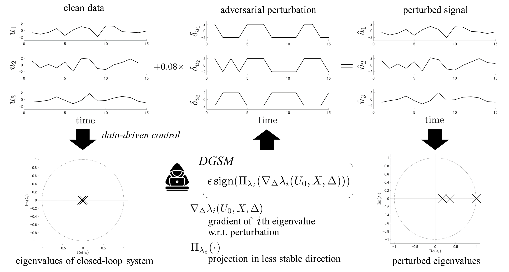
Our first contribution is to demonstrate the vulnerability of direct data-driven control. We introduce a specific attack, which we refer to as the directed gradient sign method (DGSM), based on the fast gradient sign method (FGSM), which has originally been developed for efficient computation of a severe adversarial perturbation in image classification [10]. The idea behind FGSM is to calculate the perturbation vector in the direction of the gradient of the cost function while limiting each element’s absolute value to a specified small constant. DGSM is an adaptation of this method, designed to destabilize the targeted control system. DGSM calculates the gradient of the eigenvalues of the resulting closed-loop system and determines the perturbation in the direction that makes the system less stable. Fig. 1 illustrates a demonstration of DGSM applied to a discrete-time linear system. It is shown that while the system can be stabilized by using clean data where the resulting eigenvalues are far from the unit circle it can be made unstable by a small but sophisticated perturbation.
Second, we investigate defense methods using regularization. We consider two regularization approaches: the first is the certainty-equivalence regularization that links the direct data-driven control with the indirect one via system identification using the ordinary least-square estimation [21, 22]. The second is the robustness-inducing regularization that ensures robustness against noise [8]. We demonstrate that both approaches can improve robustness against adversarial attacks and compare their effectiveness.
Organization and Notation
The paper is organized as follows. Sec. II reviews key concepts of direct data-driven control based on the fundamental lemma and discusses a technique for generating adversarial perturbations used in image classification with neural networks. In Sec. III, we outline the attack scenario and present the adversarial method adapted for direct data-driven control that leads to destabilization. Sec. IV provides experimental evaluation to discuss the vulnerabilities of interest and the improvement in robustness through regularization. Finally, Sec. V concludes and summarizes the paper.
We denote the transpose of a matrix by , the trace and the spectrum of a square matrix by and , respectively, the maximum and minimum singular values of a matrix by and respectively, the max norm of a matrix by , the right inverse of a right-invertible matrix by , the positive and negative (semi)definiteness of a Hermetian matrix by () and () , respectively, and the component-wise sign function by .
II PRELIMINARY
II-A Data-Driven Control based on Fundamental Lemma
We first review the direct data-driven control based on the Willems’ fundamental lemma [7]. Consider a discrete-time linear time-invariant system for where is the state, is the control input, and is the exogenous disturbance. Assume that the pair is unknown to the controller designer but it is stabilizable. We consider the linear quadratic regulator (LQR) problem [23, Chap. 6], which has widely been studied as a benchmark problem. Specifically, design a static state-feedback control that minimizes the cost function with and where is the th canonical basis vector. It is known that the cost function can be rewritten as where is the controllability Gramian of the closed-loop system when is Schur.
The objective of direct data-driven control is to design the optimal feedback gain using data of input and output signals without explicit system identification. Assume that the time series and are available. The first and last -long time series of are denoted by and respectively. Letting we have the relationship
where . We here assume that holds. This rank condition, which is generally necessary for data-driven LQR design [24], is satisfied if the input signal is persistently exciting in the noiseless case as shown by the Willems’ fundamental lemma [25].
The key idea of the approach laid out in [7] is to parameterize the controller using the available data by introducing a new variable with the relationship
| (1) |
Then the closed-loop matrix can be parameterized directly by data matrices as The LQR controller design can be formulated as
| (2) |
by disregarding the noise term.
However, it has been revealed that the formulation (2) is not robust to disturbance [21]. To enhance robustness against disturbance, a regularized formulation has been proposed:
| (3) |
with a constant where and is any matrix norm. The regularizer is referred to as certainty-equivalence regularization because it leads to the controller equivalent to the certainty-equivalence indirect data-driven LQR with least-square estimation of the system model when is sufficiently large [21]. Meanwhile, another regularization that can guarantee robustness has been proposed:
| (4) |
with a constant . The regularizer plays the role to reduce the size of the matrix to achieve the actual stability requirement using the constraint . We refer to the latter one as robustness-inducing regularization. For reformulation of (2), (3), and (4) into convex programs, see [26].
II-B Fast Gradient Sign Method
The fast gradient sign method (FGSM) is a method to efficiently compute an adversarial perturbation for a given image [10]. Let be the loss function of the neural network where is the input image, is the label, and is the trained parameter, and let be the trained classification model. The objective of the adversary is to cause misclassification by adding a small perturbation such that . Specifically, the max norm of the perturbation is restricted, i.e., with a small constant .
The core idea of FGSM is to choose a perturbation that locally maximizes the loss function. The linear approximation of the loss function with respect to is given by
| (5) |
where the subscript denotes the component. The right-hand side of (5) is maximized by choosing , whose matrix form is given by
FGSM creates a series of perturbations in the form increasing until misclassification occurs. In the next section, we apply this idea to adversarial attacks on direct data-driven control for destabilization.
III ADVERSARIAL ATTACKS to DIRECT DATA-DRIVEN CONTROL
III-A Threat Model
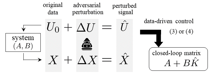
This study considers the following threat model: The adversary can add a perturbation to the input and output data . Additionally, the adversary knows the system model , the data , and the controller design algorithm. This scenario is depicted in Fig. 2. The controller is designed using the perturbed data , which results in the closed-loop matrix . The attack objective is to destabilize the system by crafting a small perturbation such that the closed-loop matrix has an eigenvalue outside the unit circle.
Additionally, we consider gray-box attacks where the adversary has access to the system model and the controller design algorithm but not the data , and additionally may not know the design parameters and . In this case, a reasonable attack strategy is to use hypothetical input and disturbance and calculate the corresponding state trajectory . We refer to effectiveness of the attack without knowledge of the data as the transferability across data. Additionally, when the design parameters are unknown, hypothetical design parameters or are also used. We refer to the effectiveness in this scenario as the transferability across parameters. We numerically evaluate the transferability properties in Sec. IV.
III-B Directed Gradient Sign Method
We develop the directed gradient sign method (DGSM) to design a severe perturbation that satisfies with a small constant . Let
denote the eigenvalues of the closed-loop system with the direct data-driven control (3) or (4) using the perturbed data . The aim of the attack is to place some element of outside the unit circle.
The core idea of DGSM is to choose a perturbation that locally shifts an eigenvalue in the less stable direction. We temporarily fix the eigenvalue of interest, denoted by , and denote its gradient with respect to by . The linear approximation of the eigenvalue with respect to is given by
| (6) |
We choose such that the right-hand side of (6) moves closer to the unit circle. Specifically, DGSM crafts the perturbation
where is defined by
| (7) |
with
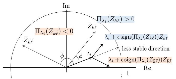
The role of the function is illustrated in Fig. 3. Suppose that faces the direction of . More precisely, the angle between and , denoted by , is less than , which leads to . We now suppose that the angle between and another element , denoted by , is greater than . Then we have . In both cases, owing to the function the perturbed eigenvalue moves closer to the unit circle as depicted in the figure. By aggregating all components, the linear approximation of the perturbed eigenvalue is given by
which is expected to be placed outside the unit circle by increasing .
DGSM performs the procedure above for every for increasing until the resulting system is destabilized. Its algorithm is summarized in Algorithm 1, where denotes possible candidates of the constant in the ascending order. Algorithm 1 finds a perturbation with the smallest in such that the resulting closed-loop system becomes unstable.
IV NUMERICAL EXPERIMENTS
IV-A Experimental Setup
We evaluate our adversarial attacks through numerical experiments. We consider the inverted pendulum [27] with sampling period whose system matrices are given by
We set the weight matrices to and . The input signal is randomly and independently generated by . We consider the disturbance-free case, i.e., . The time horizon is set to . The -induced norm is taken as the matrix norm in (3). The gradient is computed by the central difference approximation [28, Chapter 4].
IV-B Robustness Improvement by Regularization
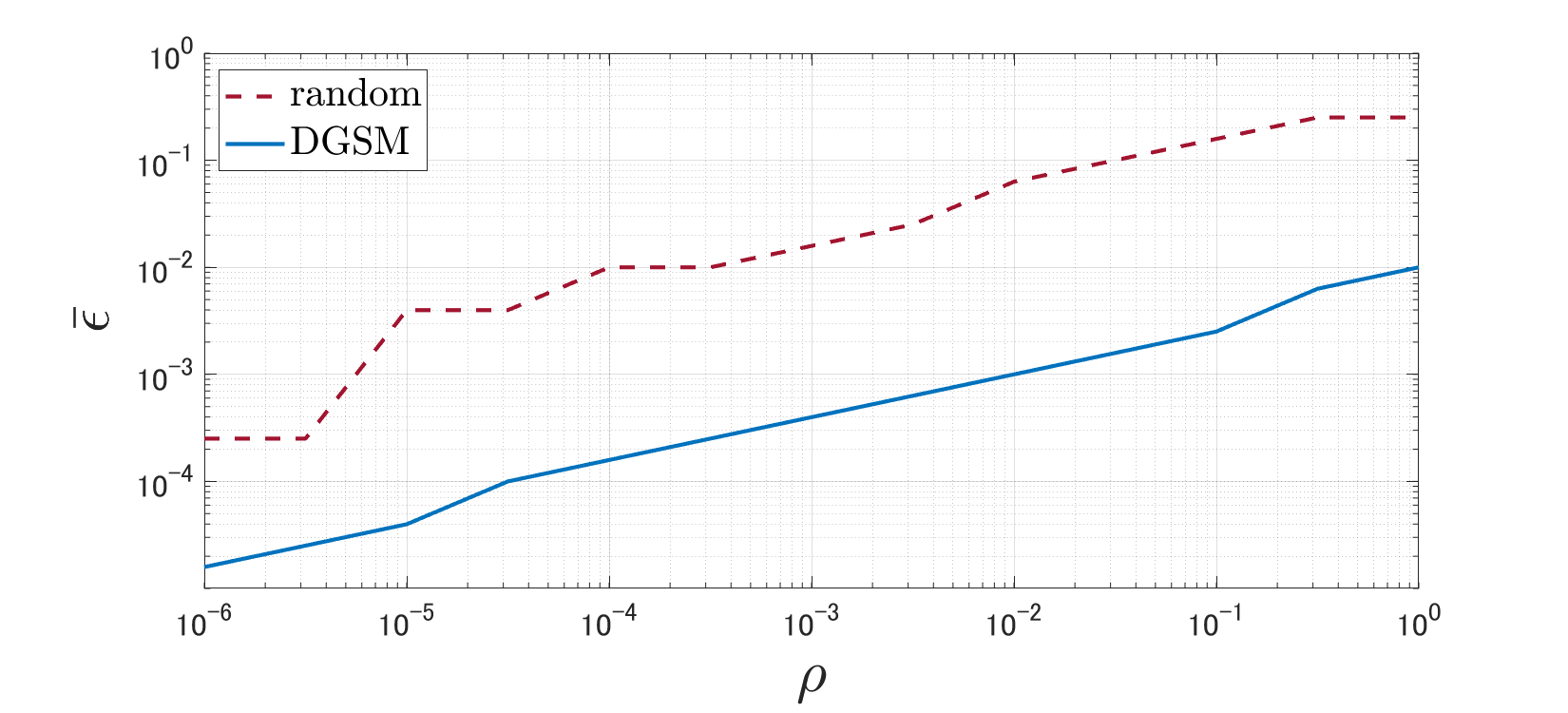
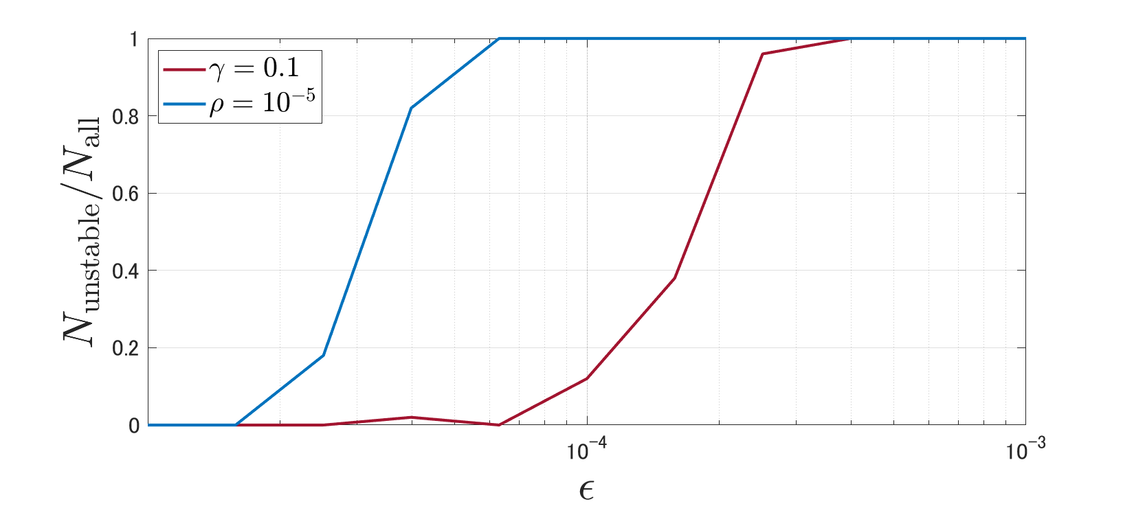
We examine the improvement in robustness through regularization by comparing DGSM with a random attack where each element of takes or with equal probability. Let and denote the total number of samples and the number of the samples where the resulting closed-loop system is unstable, respectively. In addition, let denote the minimum such that for a given threshold . We set and .
Fig. 4 depicts the curves of with varying for DGSM and the random attack when using the certainty-equivalence regularization (3). First, it is observed that the magnitude of the adversarial perturbation necessary for destabilization increases as the regularization parameter increases. This result implies that the regularization method originally proposed for coping with disturbance is also effective in improving robustness against adversarial attacks. Second, the necessary magnitude in DGSM is approximately of that in the random attack, which illustrates the significant impact of DGSM.
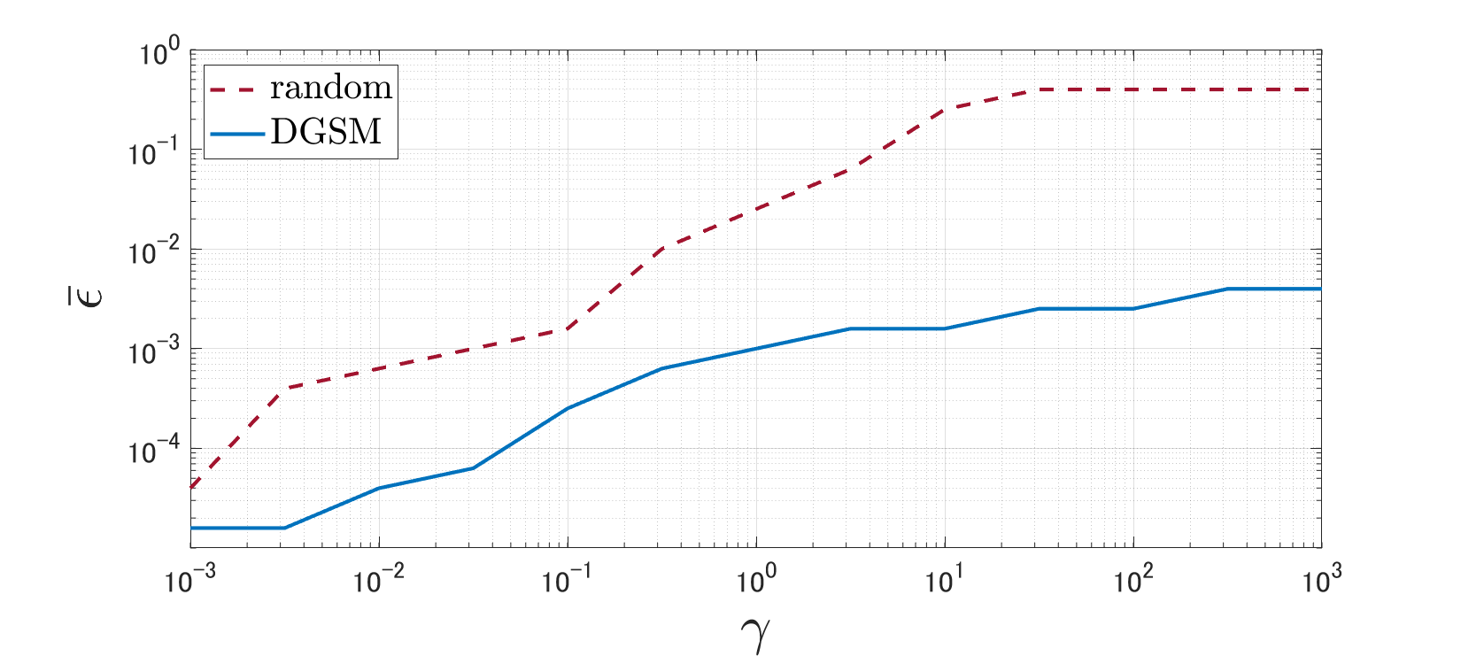
Fig. 5 depicts the curves of with varying when using the robustness-inducing regularization (4). This figure shows results similar to Fig. 4. Consequently, both regularization methods are effective for adversarial attacks.
Next, we compare the effectiveness of the two regularization methods. We take and such that the resulting closed-loop performances are almost equal. Fig. 6 depicts with the two regularized controller design methods (3) and (4) for varying . It can be observed that the robustness-inducing regularization (4) always outperforms the certainty-equivalence regularization (3).
IV-C Transferability
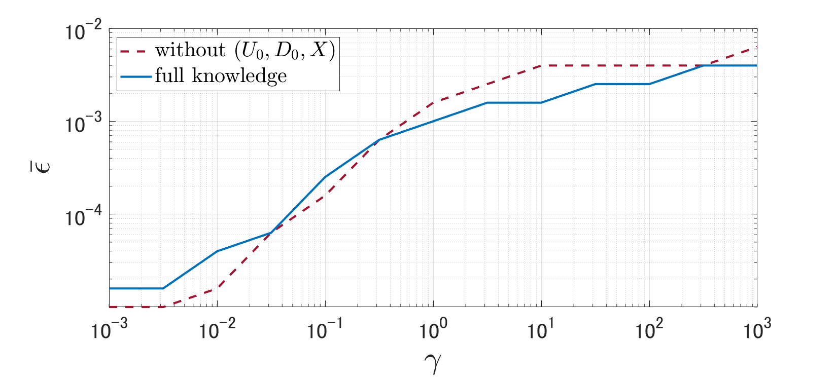
We consider transferability across data where the data is unknown and DGSM uses a hypothetical input whose elements are also randomly and independently generated by and . Fig. 7 depicts the curves of with varying for DGSM without knowledge of data and that with full knowledge when using the certainty-equivalence regularization (3). This figure shows that DGSM exhibits the transferability property across data.
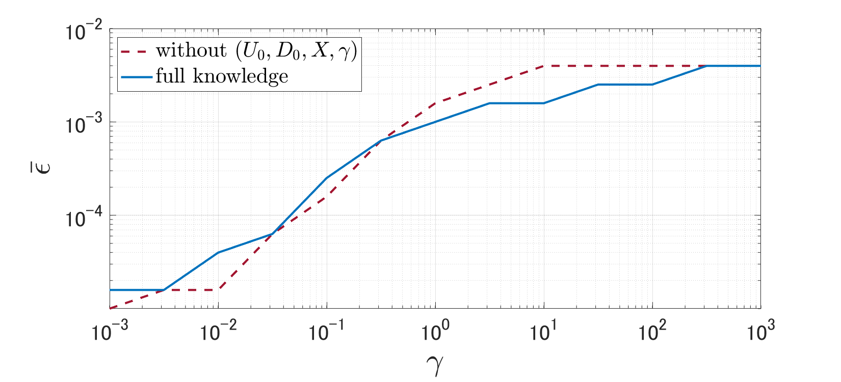
Subsequently, we examine transferability across design parameters where the regularization parameter in addition to the data is unknown. We use as a hypothetical parameter. Fig. 8 depicts the corresponding curves As in the transferability across data, the results confirm the transferability property across parameters.
IV-D Discussion
The regularization methods described by (3) and (4) provide a quantitative condition to ensure stability: The resulting closed-loop system with the certainty-equivalence regularization is stable when and the signal-to-noise ratio (SNR) defined by are sufficiently large [26, Theorem 4.2]. That with the robustness-inducing regularization is stable when is sufficiently large and is sufficiently small [8, Theorem 3]. One may expect that DGSM crafts a severe input perturbation such that its maximum singular value is large but its elements are small. However, for the single-input system, for any whose elements take or . This means that the input perturbations made by DGSM and the random attack have the same maximum singular value.
V CONCLUSION
This study has investigated the vulnerability of direct data-driven control, specifically focusing on the Willems’ fundamental lemma-based approach with two regularization methods, namely certainty-equivalence regularization and robustness-inducing regularization. To this end, a new method called DGSM, based on FGSM which has been originally been proposed for neural networks, has been introduced. It has been demonstrated that direct data-driven control can be vulnerable, i.e., the resulting closed-loop system can be destabilized by a small but sophisticated perturbation. Numerical experiments have indicated that strengthening regularization enhances robustness against adversarial attacks.
Future research should include further tests of the vulnerability with various types of data and systems under different operating conditions, a theoretical analysis of DGSM, and exploration of novel defense techniques for reliable direct data-driven control. For example, detection of adversarial perturbations [29] is a promising direction. Finally, for a more comprehensive understanding of the vulnerability, more sophisticated attacks should be considered.
The parameters in the simulation in Fig. 1 are as follows. The system is a marginally unstable Laplacian system considered in [21, 30]. Each element of the disturbance is randomly generated from with . The weight matrices are and . The time horizon is set to . The magnitude of the adversarial perturbation is set to . The controller is designed using the certainty-equivalence regularization (3) with a regularization parameter .
References
- [1] B. R. Kiran, I. Sobh, V. Talpaert, P. Mannion, A. A. A. Sallab, S. Yogamani, and P. Pérez, “Deep reinforcement learning for autonomous driving: A survey,” IEEE Trans. Intell. Transp. Syst., vol. 23, no. 6, pp. 4909–4926, 2022.
- [2] N. C. Luong, D. T. Hoang, S. Gong, D. Niyato, P. Wang, Y.-C. Liang, and D. I. Kim, “Applications of deep reinforcement learning in communications and networking: A survey,” IEEE Commun. Surv. Tutor., vol. 21, no. 4, pp. 3133–3174, 2019.
- [3] D. Silver, A. Huang, C. J. Maddison, A. Guez, L. Sifre, G. Van Den Driessche, J. Schrittwieser, I. Antonoglou, V. Panneershelvam, M. Lanctot et al., “Mastering the game of Go with deep neural networks and tree search,” Nature, vol. 529, no. 7587, pp. 484–489, 2016.
- [4] M. C. Campi and S. M. Savaresi, “Direct nonlinear control design: The virtual reference feedback tuning (VRFT) approach,” IEEE Trans. Autom. Control, vol. 51, no. 1, pp. 14–27, 2006.
- [5] F. L. Lewis and D. Liu, Reinforcement learning and approximate dynamic programming for feedback control. John Wiley & Sons, 2013.
- [6] H. Mohammadi, A. Zare, M. Soltanolkotabi, and M. R. Jovanović, “Convergence and sample complexity of gradient methods for the model-free linear–quadratic regulator problem,” IEEE Trans. Autom. Control, vol. 67, no. 5, pp. 2435–2450, 2021.
- [7] C. De Persis and P. Tesi, “Formulas for data-driven control: Stabilization, optimality, and robustness,” IEEE Trans. Autom. Control, vol. 65, no. 3, pp. 909–924, 2019.
- [8] ——, “Low-complexity learning of linear quadratic regulators from noisy data,” Automatica, vol. 128, no. 109548, 2021.
- [9] J. Bruna, C. Szegedy, I. Sutskever, I. Goodfellow, W. Zaremba, R. Fergus, and D. Erhan, “Intriguing properties of neural networks,” in International Conference on Learning Representations, 2014.
- [10] I. Goodfellow, J. Shlens, and C. Szegedy, “Explaining and harnessing adversarial examples,” in International Conference on Learning Representations, 2015.
- [11] N. Akhtar and A. Mian, “Threat of adversarial attacks on deep learning in computer vision: A survey,” IEEE Access, vol. 6, pp. 14 410–14 430, 2018.
- [12] N. Carlini, P. Mishra, T. Vaidya, Y. Zhang, M. Sherr, C. Shields, D. Wagner, and W. Zhou, “Hidden voice commands,” in 25th USENIX security symposium (USENIX security 16), 2016, pp. 513–530.
- [13] S. Huang, N. Papernot, I. Goodfellow, Y. Duan, and P. Abbeel, “Adversarial attacks on neural network policies,” in International Conference on Learning Representations, 2017.
- [14] F. Pasqualetti, F. Dörfler, and F. Bullo, “Control-theoretic methods for cyberphysical security: Geometric principles for optimal cross-layer resilient control systems,” IEEE Control Systems Magazine, vol. 35, no. 1, pp. 110–127, 2015.
- [15] J. Giraldo et al., “A survey of physics-based attack detection in cyber-physical systems,” ACM Comput. Surv., vol. 51, no. 4, 2018.
- [16] P. Griffioen, S. Weerakkody, and B. Sinopoli, “A moving target defense for securing cyber-physical systems,” IEEE Trans. Autom. Control, vol. 66, no. 5, pp. 2016–2031, 2020.
- [17] R. Alisic and H. Sandberg, “Data-injection attacks using historical inputs and outputs,” in 2021 European Control Conference (ECC), 2021, pp. 1399–1405.
- [18] R. Alisic, J. Kim, and H. Sandberg, “Model-free undetectable attacks on linear systems using LWE-based encryption,” IEEE Control Syst. Lett., 2023.
- [19] V. Krishnan and F. Pasqualetti, “Data-driven attack detection for linear systems,” IEEE Control Syst. Lett., vol. 5, no. 2, pp. 671–676, 2020.
- [20] C. Szegedy, W. Zaremba, I. Sutskever, J. Bruna, D. Erhan, I. Goodfellow, and R. Fergus, “Intriguing properties of neural networks,” in International Conference on Learning Representations, 2014.
- [21] F. Dörfler, P. Tesi, and C. De Persis, “On the role of regularization in direct data-driven LQR control,” in 2022 IEEE 62nd Conference on Decision and Control (CDC), 2022, pp. 1091–1098.
- [22] F. Dorfler, J. Coulson, and I. Markovsky, “Bridging direct & indirect data-driven control formulations via regularizations and relaxations,” IEEE Trans. Autom. Control, 2022.
- [23] T. Chen and B. A. Francis, Optimal sampled-data control systems. Springer, 2012.
- [24] H. J. Van Waarde, J. Eising, H. L. Trentelman, and M. K. Camlibel, “Data informativity: A new perspective on data-driven analysis and control,” IEEE Trans. Autom. Control, vol. 65, no. 11, pp. 4753–4768, 2020.
- [25] J. C. Willems, P. Rapisarda, I. Markovsky, and B. L. De Moor, “A note on persistency of excitation,” Systems & Control Letters, vol. 54, no. 4, pp. 325–329, 2005.
- [26] F. Dörfler, P. Tesi, and C. De Persis, “On the certainty-equivalence approach to direct data-driven LQR design,” 2021, [Online]. Available: https://arxiv.org/pdf/2109.06643.pdf.
- [27] P. Chalupa and V. Bobál, “Modelling and predictive control of inverted pendulum,” in 22nd European Conference on Modelling and Simulation, vol. 3, no. 6, 2008, pp. 531–537.
- [28] R. L. Burden, J. D. Faires, and A. M. Burden, Numerical Analysis, 10th ed. Cengage learning, 2015.
- [29] J. H. Metzen, T. Genewein, V. Fischer, and B. Bischoff, “On detecting adversarial perturbations,” in International Conference on Learning Representations, 2017.
- [30] S. Dean, H. Mania, N. Matni, B. Recht, and S. Tu, “On the sample complexity of the linear quadratic regulator,” Foundations of Computational Mathematics, vol. 20, no. 4, pp. 633–679, 2020.