AdvantageNAS: Efficient Neural Architecture Search with Credit Assignment
Abstract
Neural architecture search (NAS) is an approach for automatically designing a neural network architecture without human effort or expert knowledge. However, the high computational cost of NAS limits its use in commercial applications. Two recent NAS paradigms, namely one-shot and sparse propagation, which reduce the time and space complexities, respectively, provide clues for solving this problem. In this paper, we propose a novel search strategy for one-shot and sparse propagation NAS, namely AdvantageNAS, which further reduces the time complexity of NAS by reducing the number of search iterations. AdvantageNAS is a gradient-based approach that improves the search efficiency by introducing credit assignment in gradient estimation for architecture updates. Experiments on the NAS-Bench-201 and PTB dataset show that AdvantageNAS discovers an architecture with higher performance under a limited time budget compared to existing sparse propagation NAS. To further reveal the reliabilities of AdvantageNAS, we investigate it theoretically and find that it monotonically improves the expected loss and thus converges.
1 Introduction
Deep neural networks (DNNs) have achieved remarkable performance improvements in various domains. Finding a suitable DNN architecture is critical for applying a DNN to a new task and achieving higher performance. However, as the architecture is defined by a combination of tens to hundreds of hyperparameters (filter sizes of convolutional layers, existence of connections between some layers, etc.), improving such a combination requires considerable human effort and expert knowledge. Neural architecture search (NAS) has been studied as a promising approach for automatically identifying sophisticated DNN architectures and overcoming the problems in applying DNNs to previously unseen tasks.
However, the high computational cost (time and space complexity) of NAS is a bottleneck in its applications, especially commercial applications that do not involve multiple high-spec GPUs. Hence, reducing the computational cost of NAS is an important research direction.
One-shot NAS reduces the time complexity of NAS by simultaneously optimizing the architecture and the parameters (weights) in a single training process or a few training processes. It maintains a redundant deep learning model comprising numerous layers and connections, called the parent network, which can represent all possible architectures in the search space as its sub-network. All the parameters required by candidate architectures are possessed by the parent network and shared among different architectures. The goodness of an architecture is evaluated using the shared parameters, which drastically reduces the computational time for the architecture search compared to conventional approaches that require the parameters to be trained from scratch for each candidate architecture evaluation.
From the viewpoint of GPU memory consumption, one-shot NAS can be categorized into dense propagation NAS (DP-NAS) and sparse propagation NAS (SP-NAS). DP-NAS requires the entire parent network to be loaded in the GPU memory to perform forward and/or backward propagation, whereas SP-NAS requires only a sub-network to be loaded. DP-NAS is more popular owing to the success of DARTS and its successors (Liu, Simonyan, and Yang 2019; Xie et al. 2019; Yao et al. 2020). However, because of its high memory consumption, its search space is limited. SP-NAS overcomes this limitation and provides more flexible search spaces on a standard GPU with limited memory. Hence, we focus on SP-NAS in this study.
To further reduce the computational cost of one-shot SP-NAS, we propose a novel one-shot SP-NAS, namely AdvantageNAS. Although various factors affect the performance of NAS (performance estimation, search space, etc.) and state-of-the-art (SOTA) performance may require a search for the best combination of these factors, this study focuses on the search strategy. We emphasize that the objective of this study is not to obtain the SOTA architecture but to investigate the efficiency of the search strategy.
AdvantageNAS is a gradient-based SP-NAS.111The advantages of gradient-based approaches are as follows. Approaches using evolutionary algorithms (e.g., (Real et al. 2017)) or progressive search methods (e.g., (Liu et al. 2018)) must define a mutation or expansion strategy depending on the search space. Such manual preparations depending on the search space are not required in gradient-based methods. Another advantage of gradient-based methods is that they can be easily implemented in most modern deep learning frameworks, as they support automatic differentiation of deep neural networks. This category of NAS includes ENAS (Pham et al. 2018), ProxylessNAS (Cai, Zhu, and Han 2019), PARSEC (Casale, Gordon, and Fusi 2019), and GDAS (Dong and Yang 2019). These methods introduce a family of parametric probability distributions from which an architecture is sampled, and the distribution parameter is updated with a gradient of the objective function estimated using the Monte Carlo method, which indirectly optimizes the architecture itself. As the gradient is estimated, reducing the variance of the gradient estimate intuitively improves the search efficacy. Inspired by the actor-critic approach (Konda and Tsitsiklis 2000), we adopt the notion of advantage, which has been introduced to solve the well-known credit assignment problem of policy gradients (Minsky 1961).
We investigate AdvantageNAS both theoretically and empirically. Empirical studies show that it performs well on different tasks with different search spaces, whereas theoretical studies guarantee its performance on empirically unforeseen tasks. Theoretical studies are relatively scarce in NAS research; however, they are important for investigating search strategies for NAS.
Our contributions are summarized as follows:
-
•
We propose a novel SP-NAS, namely AdvantageNAS. Our analysis of a test scenario demonstrates that the estimation variance of the gradient is reduced compared to REINFORCE (Williams 1992), which is a baseline search strategy for ENAS.
-
•
The theoretical investigation reveals that the estimated gradient in AdvantageNAS is an unbiased estimator of the gradient of the expected loss. From the unbiasedness, we find that AdvantageNAS monotonically improves the expected loss and thus converges. Further, we confirm that reducing the gradient variance contributes to an improved lower bound of the loss improvement in each iteration.
-
•
We compared AdvantageNAS with various gradient-based NAS methods in three different settings to demonstrate its efficacy on different search spaces. Our experiments were performed on the same code base to compare the search strategies.222NAS approaches using different components such as search spaces and training protocols have been compared in the literature. However, it has been reported, e.g., in (Yang, Esperança, and Carlucci 2020), that such differences in the components make it difficult to fairly compare the contributions of each component. Our code: https://github.com/madoibito80/advantage-nas. The results showed that AdvantageNAS converges faster than existing SP-NAS approaches.
2 One-shot Neural Architecture Search
DAG Representation of DNNs
We formulate a deep neural network as a directed acyclic graph (DAG) following previous studies (Pham et al. 2018; Liu, Simonyan, and Yang 2019). In the DAG representation, each node corresponds to a feature tensor and each edge corresponds to an operation applied to the incoming feature tensor, e.g., convolution or pooling. The adjacency matrix of the DAG is pre-defined. Let be a set of edges. The input and output nodes are two special nodes; the feature tensor at the input node is the input to the DNN and the input node has no incoming edge, while the feature tensor at the output node is the output of the DNN and the output node has no outgoing edge.
The feature tensor at node , except for the input node, is computed as follows. Let be a subset of the edges that point to node . Let be the input node of edge . For each edge , the operation is applied to and output . The feature tensor is computed by aggregating the outputs of the incoming edges with some pre-defined aggregation function such as summation or concatenation.
Search Space for Neural Architecture
For each edge of the DAG, a set of candidate operations is prepared. Let be the indices of the candidate operations at edge , and each candidate operation is denoted as for . Each candidate operation may have its own real-valued parameter vector , often referred to as a weights, and is assumed to be differentiable w.r.t. the weights. The operation of edge is then defined as a weighted average of the candidate operations with weight :
| (1) |
where . The vector is referred to as the architecture.
The objective of NAS is to locate the best architecture under some performance criterion. The aim of our study, as well as many related studies (Liu, Simonyan, and Yang 2019; Xie et al. 2019; Cai, Zhu, and Han 2019; Dong and Yang 2019; Yao et al. 2020; Casale, Gordon, and Fusi 2019), is to find the best architecture such that for each is a one-hot vector. In other words, we choose one operation at each edge.
Weight Sharing and One-shot NAS
One-shot architecture search is a method for jointly optimizing and during a single training process.
Let be a performance metric (referred to as reward in this study) that takes an architecture and weights required to compute the DAG defined by . The reward is typically the negative expected loss , where is a data-wise loss, is a data distribution, and represents data. For example, in the image classification task, is a set of an image and its label, and is the cross-entropy loss using . The objective of NAS is written as , where is the optimal weights for architecture . The expected reward is often approximated by the average over the validation dataset for optimization of and the training dataset for optimization of . The difficulty in simultaneously optimizing and is that the domain of changes with during the training process. The time complexity of conventional NAS approaches (e.g., (Zoph and Le 2017)) is extremely high because they require to be trained for each from scratch.
Weight sharing (Pham et al. 2018) is a technique for simultaneous optimization. All the weights appearing in the candidate operations are stored in a single weight set, . The reward function is extended to accept by defining . Then, the objective of NAS is to find that maximizes . A disadvantage of the weight sharing approach is that a large parameter set is required during the search. However, this set can be stored in the CPU memory and only a subset is required to be loaded in the GPU, which typically involves much smaller memory. Moreover, if is sparse during the training, the GPU memory consumption is limited.
3 Gradient-based One-shot NAS
| Method | Propagation | Stochastic | TG | |
|---|---|---|---|---|
| DARTS | dense | n-hot | no | |
| SNAS | dense | n-hot | yes | |
| NASP | dense333NASP performs sparse propagation in the weight update step and dense propagation in the architecture update step. | 1-hot | no | ✓ |
| ProxylessNAS | sparse | 2-hot | yes | |
| PARSEC | sparse | 1-hot | yes | |
| GDAS | sparse | 1-hot | yes | |
| ENAS | sparse | 1-hot | yes | |
| AdvantageNAS | sparse | 1-hot | yes | ✓ |
The major stream of search strategies for one-shot NAS is gradient-based search (Pham et al. 2018; Liu, Simonyan, and Yang 2019; Xie et al. 2019; Cai, Zhu, and Han 2019; Dong and Yang 2019; Yao et al. 2020; Casale, Gordon, and Fusi 2019). The architecture is either re-parameterized by a real-valued vector through some function or sampled from a probability distribution parameterized by . Gradient steps on as well as on are taken alternatively or simultaneously to optimize and .
A comparison of related studies is shown in Table 1.
Dense Propagation NAS (DP-NAS)
DP-NAS has been popularized by DARTS (Liu, Simonyan, and Yang 2019), where the architecture is re-parameterized by the real-valued vector through the softmax function , where and
| (2) |
In other words, the output of the th edge in (1) is a weighted sum of the outputs of all candidate operations. The architecture is optimized with the gradient .
Sparse Propagation NAS (SP-NAS)
SP-NAS introduces a parametric probability distribution over the architecture space and optimizes indirectly through the optimization of . Thus, all of the SP-NAS is the stochastic algorithm shown in Table 1. The objective is to maximize the reward function expected over the architecture distribution . Different distributions and different update rules have been proposed. ENAS (Pham et al. 2018) uses LSTM (Hochreiter and Schmidhuber 1997) to represent and REINFORCE (Williams 1992) to estimate :
| (3) |
Note that REINFORCE does not need to execute a backward process to update and (3) can be approximated using the Monte Carlo method with .
Different follow-up studies have been conducted to accelerate the optimization of . PARSEC (Casale, Gordon, and Fusi 2019) replaces LSTM with a categorical distribution, where is a probability vector. ProxylessNAS (Cai, Zhu, and Han 2019) and GDAS (Dong and Yang 2019) aim to incorporate the gradient information rather than a single reward value to update , as in the case of DP-NAS. To avoid dense architecture evaluation, they require different approximation techniques ((Courbariaux, Bengio, and David 2015) and (Maddison, Mnih, and Teh 2017), respectively) and the resulting parameter update procedures require only sparse architecture evaluation.
Characteristics of DP-NAS and SP-NAS
The dense forward or backward propagation is a major drawback of DP-NAS. The forward propagation results of all the candidate operations at all the edges need to be obtained to compute . Thus, the GPU memory consumption in each iteration is approximately proportional to , which prevents the construction of a large parent network.
A popular approach for overcoming this limitation is to optimize the architecture of a smaller network on a proxy task (Zoph et al. 2018) consisting of a similar to the original dataset but smaller one. For example, CIFAR (Krizhevsky 2009) is used as a proxy task for ImageNet (Deng et al. 2009). The obtained architecture is expanded by repeating it or increasing the number of nodes to construct a larger network. Approaches based on proxy tasks rely on transferability. However, the architectures obtained on the proxy task do not necessarily perform well on other tasks (Dong and Yang 2020). In addition, constructing a proxy task for DP-NAS requires human effort, and the incurred cost prevents practitioners from using NAS in commercial applications.
The advantage of SP-NAS over DP-NAS is that it needs to perform forward (and backward) propagation only in one operation at each edge. Therefore, its GPU memory consumption in each iteration is independent of the number of operations at each edge. As its GPU memory consumption is comparable to that of a single architecture, it does not need any proxy task even when a search space designed for a task requires a large parent network. The advantage of such a search space with a large parent network is demonstrated by, for example, ProxylessNAS (Cai, Zhu, and Han 2019), which achieves SOTA accuracy on ImageNet under mobile latency constraints.
4 AdvantageNAS
We propose a novel search strategy for one-shot SP-NAS. Inspired by the credit assignment problem of policy gradients, we improve the convergence speed of the REINFORCE algorithm, i.e., the baseline search strategy for ENAS, by introducing the so-called advantage function. As with other SP-NAS, our proposed approach, AdvantageNAS, has low GPU memory consumption.
4.1 Framework
The probability distribution for is modeled by an independent categorical distribution. Each for independently follows a categorical distribution parameterized by . The probability mass function for is written as the product , where . The domain of is and the probability of being in the th category is defined by (2).
The objective function of AdvantageNAS is the reward function expected over the architecture distribution, i.e., , similar to REINFORCE. It is easy to see that the maximization of leads to the maximization of since and , where represents the Dirac delta function concentrated at .
AdvantageNAS update and alternately. The weights is updated by estimating the gradient using the Monte Carlo method with an architecture sample and a minibatch reward , where . Then, is updated by estimating the policy gradient using the Monte Carlo method with another architecture sample and a minibatch reward , where . Next, we discuss how to estimate the policy gradient to improve the convergence speed while maintaining the time and space complexities at levels similar to those in previous studies. The algorithm of AdvantageNAS is described in Algorithm 1 using pseudocode.
4.2 Estimation Variance of Policy Gradient
The REINFORCE algorithm estimates the gradient using a simple Monte Carlo method,
| (4) |
where is an architecture sampled from . In general, this gradient is called a policy gradient, where is regarded as a policy that takes no input (i.e., no state) and outputs the probability of selecting each architecture (as an action). For our choice of , the gradient of the log-likelihood is . In other words, the probability vector is updated to approach if the minibatch reward is positive. A higher reward results in a greater shift of towards current sample .
Intuitively, a high estimation variance will lead to slow convergence. This is indeed theoretically supported by the subsequent result, whose proof follows (Akimoto et al. 2012); the details are presented in Section A.1. The lower the estimation variance of policy gradient , the greater is the lower bound of the expected improvement in one step. Therefore, reducing the estimation variance is key to speed up the architecture update.
Theorem 4.1.
Let and be an unbiased estimator of . Suppose that for any . Then, for any ,
| (5) |
Credit assignment in reinforcement learning tasks is a well-known cause of slow convergence of policy gradient methods (Minsky 1961). The reward is the result of a set of consecutive actions (in our case, the choice at each edge ). A positive reward for does not necessarily mean that all the actions are promising. However, since (4) updates based on a single reward, it cannot recognize the contribution of each edge. To understand this problem, consider a situation in which we have two edges with two candidate operations for each edge. The reward is assumed to be the sum of the contributions of the choices on the two edges, for for and and and . If and , i.e., the contribution of the first edge dominates, the sign of the reward is determined by . The update direction of is determined by ; it is not based on whether is a better choice. This results in a high variance for the update, leading to slow convergence.
4.3 Advantage
We introduce the notion of advantage, used in policy gradient methods, to address the issue of credit assignment (Minsky 1961). We regard as a state and as an action. By introducing the advantage, we evaluate the goodness of the choice at each edge rather than evaluate the goodness of successive actions by a scalar reward . We expect to reduce the estimation variance of the policy gradient by the advantage.
We define the advantage of as (by letting )
| (6) |
It is understood as follows. Given the state , the advantage of the action is the rewards improvement over , where the output of the th edge is zero.444When a zero operation (returns zero consistently) is included in the search space, we replace the advantage of the zero operation with the worst expected advantage of the other operations estimated by a moving average. The rationale for this modification is as follows. First, (6) for the zero operation is always zero, resulting in no architecture update, which is not preferred. Second, the zero operation can mostly be represented by other operations with specific weights. Hence, there is no reason to prefer it unless we consider a latency constraint. See Appendix B for further details. We replace the reward with the advantage in the policy gradient estimation in (4). If we replace the second term on the right-hand side of (6) with a single scalar independent of , the resulting policy gradient is known to be an unbiased estimator (Evans and Swartz 2000). However, a state-dependent advantage such as (6) is not unbiased in general. The following result states that the policy gradient estimate using this advantage is an unbiased estimate of (4). Its proof is presented in Section A.2.
Theorem 4.2.
Let and be i.i.d. from . Then, with defined in (6), is an unbiased estimate of , i.e., .
Thus, we can use different advantage values rather than a single reward value. A shortcoming of the above approach is that it requires the computation of an additional reward to compute for each ; hence, it requires additional forward propagation to estimate (4). As our objective is to reduce the time complexity by improving the convergence speed of SP-NAS, we aim to compute an advantage with ideally no additional computational cost.
To reduce the computational cost, we approximate the advantage function (6) as (dropping and for short)
| (7) |
where and are as in (1) and is the index of the selected operation at edge , i.e., is the one-hot vector with at th. Also note that here we consider the situation where and are column vectors and the batch size equals 1 for simplicity. The above approximation follows the first-order Taylor approximation of the reward around . Compared to a naive policy gradient computation that uses only a single reward , the policy gradient estimate with the above approximate advantage additionally requires only one reward gradient computation, . The output of the selected operation is computed in the forward process and is computed in the backward process. Therefore, our advantage involves no additional computational cost.
AdvantageNAS uses the gradient information of the reward rather than a scalar reward. Existing works on SP-NAS also use the gradient (Cai, Zhu, and Han 2019; Dong and Yang 2019). AdvantageNAS aims to reduce the estimation variance while keeping the policy gradient unbiased, whereas the previous methods simply try to incorporate the gradient information of the reward and they do not consider the estimation bias.
4.4 Variance Reduction Effect : An Example
We know from Theorem 4.2 that the advantage (6) provides an unbiased estimator of the gradient and from Theorem 4.1 that reducing the variance in an unbiased estimator of the gradient contributes toward improving the lower bound of the expected improvement. Since (7) is an approximation of (6), we expect that our advantage contributes toward reducing the estimation variance, resulting in faster convergence.
To understand the variance reduction effect of the proposed advantage, we consider a simple situation in which the reward is given by for some vector . In this example, neither nor is introduced. In this linear objective situation, the advantages (6) and (7) are equivalent and . The square norm of the gradient component is . The estimation variance of the policy gradient using the advantage (6) or (7) is . Meanwhile, the estimation variance of the policy gradient using a reward value (i.e., (4)) is . In other words, the variance reduction effect for each gradient component typically scales linearly with (because ), whereas and do not. In light of Theorem 4.1, the proposed advantage potentially contributes toward improving the search performance, especially when the number of edges is .
5 Experiments
We performed three experiments to compare the search efficiency of AdvantageNAS with that of existing gradient-based search strategies for NAS. Note that our objective is not to obtain the SOTA architecture; hence, the search spaces used in the experiments were relatively small for convenience. To compare the search strategies for NAS fairly, we implemented all the baseline NAS methods on the same code base and imposed the same setting except for the search strategy.
5.1 Toy Regression Task
Motivation
Whereas one-shot NAS methods optimize the weights and architecture simultaneously, to solely assess the performance improvement due to the differences in the architecture updates, we evaluate the performance of the architecture optimization while the weights are fixed. In particular, we confirm that the variance reduction by our advantage contributes toward accelerating the architecture search by comparing the performance of REINFORCE and AdvantageNAS, which are different only in terms of the reward computation for each edge as described in Section 4.3.
Task Description
We prepare two networks: teacher-net and student-net . Both networks are represented by the same DAG. The two networks have intermidiate nodes, and there are edges from one input node to all the intermidiate nodes. For each edge , different convolutional filters are prepared as the candidate operations. These filters have a filter size of , stride of , and output channels of followed by activation. The architecture variable of teacher-net is such that are one-hot vectors, i.e., one convolutional filter per edge which connects the input node and the intermediate node. For each edge from an intermediate node to the output node, a convolution with filter size of , stride of , and output channels of is applied. The average of the outputs is taken as the aggregation function for the output node. A minibatch with batch size of is sampled randomly for each iteration, where the input data is generated by the uniform distribution over and its ground truth is given by . The reward function is defined as the negative loss; the squared error between the ground truth and the student prediction . The weights for the convolutions are fixed to be the same () for both networks during the architecture optimization process. The and are defined randomly before the optimization process. The loss is consistently zero if and only if student-net learns the optimal architecture . We optimize using the Adam optimizer (Kingma and Ba 2015) with a learning rate of and . The implementation details of gradient-based methods are presented in Appendix C.

Results
Figure 1 shows the results. The test loss is computed for the architecture obtained by selecting the operation at each edge such that is maximum. We observe that AdvantageNAS converges faster than existing SP-NAS such as REINFORCE, PARSEC and GDAS. Moreover, it is more stable than ProxylessNAS when the number of iterations is large. Existing DP-NAS approaches such as DARTS, SNAS and NASP converge faster than AdvantageNAS. However, as mentioned above, these methods require nearly times the memory space to perform the architecture search, which prevents their application to a large-scale task requiring a large architecture.
| Method | argmax | process best | ||
|---|---|---|---|---|
| accuracy | params(MB) | accuracy | params(MB) | |
| REINFORCE(Pham et al. 2018; Williams 1992) | ||||
| PARSEC(Casale, Gordon, and Fusi 2019) | ||||
| ProxylessNAS(Cai, Zhu, and Han 2019) | - | - | ||
| GDAS(Dong and Yang 2019) | ||||
| AdvantageNAS | ||||
5.2 Convolutional Cell on CIFAR-10

Motivation
Search Settings
The CIFAR-10 dataset contains 50000 training data and 10000 test data. We split the original training data into 25000 training data and 25000 validation data , as in the case of NAS-Bench-201. We use to optimize and to optimize . Our architecture search space is the same as NAS-Bench-201 except that the zero operations are removed.555Our preliminary experiments showed that zero operations disrupt the architecture search of existing SP-NAS (e.g., ProxylessNAS ended up with a final accuracy of ). We removed zero operations to avoid the effects of search space definition. See Appendix F for the results on the search space including the zero operations. We search for the convolutional cell architecture and stack it 15 times to construct a macro skeleton. All the stacked cells have same architecture. The cell structure has a total of edges. In each cell, there are candidate operations such as convolution, convolution, average pooling and identity map. The total procedure was conducted in 100 epochs; however, was fixed in the first 50 epochs for pre-training . The other settings are presented in Appendix D.
| Method | validation perplexity | test perplexity | params(MB) |
|---|---|---|---|
| REINFORCE(Pham et al. 2018; Williams 1992) | |||
| PARSEC(Casale, Gordon, and Fusi 2019) | |||
| ProxylessNAS(Cai, Zhu, and Han 2019) | |||
| GDAS(Dong and Yang 2019) | |||
| AdvantageNAS |
Evaluation Settings
To evaluate the performance of one-shot NAS, the weights for the architectures obtained by the search process are often retrained for longer epochs; then, the test performances are compared. To minimize the influence of the quality of retraining on the performance metric, we use NAS-Bench-201 (Dong and Yang 2020) for evaluation. It is a database containing average accuracy for all architectures in the search space. The accuracy was computed after 200 epochs of training on CIFAR-10 with each architecture. Each architecture was trained three times independently and its average accuracy is recorded in the database. We use this average accuracy for the performance metric.
There are different ways for determining the final architecture after architecture search. One way is to choose the best architecture based on its validation loss observed in the search process. This way is adopted by, e.g., ENAS (REINFORCE) and GDAS, and is denoted as process best. Another way (adopted by ProxylessNAS and PARSEC) is to take operation for which is maximum at each edge , as in Section 5.1. It is denoted as argmax. In our experiment, we show the performance of these two ways and confirmed which one is better suited for AdvantageNAS.
Results
Table 2 presents the results. AdvantageNAS achieves an improvement over REINFORCE solely owing to the introduction of the advantage described in Section 4.3. Moreover, AdvantageNAS outperforms all the existing SP-NAS in terms of both argmax and process best. Although process best was adopted in ENAS and GDAS, argmax delivered better performances in all the algorithms including AdvantageNAS. A comparison with DP-NAS is shown in Appendix G for reference.
The search progress in the initial steps is shown in Figure 2. The median of the average accuracy on NAS-Bench-201 is shown for each method with argmax over three independent search trials. At the early stage in the search process, AdvantageNAS achieved a higher accuracy than that of the existing SP-NAS and was more stable at the high accuracy. It can be inferred that AdvantageNAS outperforms the existing SP-NAS in terms of convergence speed.
To further assess the convergence speed, we analyzed the entropy of categorical distribution in the search process. The details are presented in Appendix H.
5.3 Recurrent Cell on Penn Treebank
Motivation
We confirm that the usefulness of AdvantageNAS for recurrent cell architecture search as well as for convolutional cells.
Settings
We use Penn Treebank (Marcus, Santorini, and Marcinkiewicz 1993) (PTB) dataset to search for the recurrent cell architecture. Most of the settings is the same as those of DARTS (Liu, Simonyan, and Yang 2019). See Appendix E for the details. The recurrent cell structure has edges. They have operation candidates, namely ReLU, tanh, sigmoid, identity, and zero operation, after linear transformation is applied. The parameters of the linear transformation are trainable weights. In the search process, we use the training data of PTB to optimize both the weights and for 30 epochs. Finally, the obtained architectures are retrained in 100 epochs. According to previous studies, we chose the final architecture by argmax in ProxylessNAS and PARSEC and by process best for REINFORCE(ENAS) and GDAS. The final architecture of AdvantageNAS is determined by argmax. The validation and test data of PTB are used to measure the final performance.
Results
The performances of the retrained architectures are shown in Table 3. AdvantageNAS achieved highest performance in validation data. In addition, AdvantageNAS achieved the competitive result obtained by ProxylessNAS in test data. This result implies that AdvantageNAS can be applied to various domains. The architectures obtained by AdvantageNAS and ProxylessNAS were similar, as shown in Appendix I.
6 Conclusion
We proposed AdvantageNAS, a novel gradient-based search strategy for one-shot NAS. AdvantageNAS aims to accelerate the architecture search process while maintaining the GPU memory consumption as in the case of sparse propagation NAS. For this purpose, we introduced the notion of credit assignment into the architecture search to reduce the variance of gradient estimation. A unique aspect of our study is the theoretical guarantee of the monotonic improvement of the expected loss by AdvantageNAS. Empirical evaluations were performed on different datasets and search spaces, confirming the promising performance of AdvantageNAS. To compare only the search strategies, we implemented the existing approaches on the same publicly available code base. To make an important contribution to the NAS community, we focused on investigating only the efficacy of the search strategy. Finding SOTA architectures, which requires searching for best combinations of different NAS components, is beyond the scope of this study. Further investigation of larger search spaces is an important direction for future research.
Acknowledgements
The first author would like to thank Idein Inc. for their support. This paper is partly based on the results obtained from a project commissioned by the New Energy and Industrial Technology Development Organization (NEDO).
References
- Akimoto et al. (2012) Akimoto, Y.; Nagata, Y.; Ono, I.; and Kobayashi, S. 2012. Theoretical Foundation for CMA-ES from Information Geometry Perspective. Algorithmica 64(4): 698–716. ISSN 0178-4617.
- Cai, Zhu, and Han (2019) Cai, H.; Zhu, L.; and Han, S. 2019. ProxylessNAS: Direct Neural Architecture Search on Target Task and Hardware. In ICLR.
- Casale, Gordon, and Fusi (2019) Casale, F. P.; Gordon, J.; and Fusi, N. 2019. Probabilistic Neural Architecture Search. CoRR arXiv:1902.05116.
- Courbariaux, Bengio, and David (2015) Courbariaux, M.; Bengio, Y.; and David, J.-P. 2015. BinaryConnect: Training Deep Neural Networks with binary weights during propagations. In NIPS, 3123–3131.
- Deng et al. (2009) Deng, J.; Dong, W.; Socher, R.; Li, L.; Kai Li; and Li Fei-Fei. 2009. ImageNet: A large-scale hierarchical image database. In CVPR, 248–255.
- Dong and Yang (2019) Dong, X.; and Yang, Y. 2019. Searching for A Robust Neural Architecture in Four GPU Hours. In CVPR, 1761–1770.
- Dong and Yang (2020) Dong, X.; and Yang, Y. 2020. NAS-Bench-201: Extending the Scope of Reproducible Neural Architecture Search. In ICLR.
- Evans and Swartz (2000) Evans, M.; and Swartz, T. 2000. Approximating integrals via Monte Carlo and deterministic methods. Oxford University Press.
- Hochreiter and Schmidhuber (1997) Hochreiter, S.; and Schmidhuber, J. 1997. Long Short-Term Memory. Neural Computation 9(8): 1735–1780.
- Kingma and Ba (2015) Kingma, D. P.; and Ba, J. 2015. Adam: A Method for Stochastic Optimization. In ICLR.
- Konda and Tsitsiklis (2000) Konda, V. R.; and Tsitsiklis, J. N. 2000. Actor-Critic Algorithms. In NIPS, 1008–1014.
- Krizhevsky (2009) Krizhevsky, A. 2009. Learning Multiple Layers of Features from Tiny Images. Technical report, University of Toronto.
- Liu et al. (2018) Liu, C.; Zoph, B.; Neumann, M.; Shlens, J.; Hua, W.; Li, L.; Fei-Fei, L.; Yuille, A. L.; Huang, J.; and Murphy, K. 2018. Progressive Neural Architecture Search. In ECCV, volume 11205 of Lecture Notes in Computer Science, 19–35.
- Liu, Simonyan, and Yang (2019) Liu, H.; Simonyan, K.; and Yang, Y. 2019. DARTS: Differentiable Architecture Search. In ICLR.
- Maddison, Mnih, and Teh (2017) Maddison, C. J.; Mnih, A.; and Teh, Y. W. 2017. The Concrete Distribution: A Continuous Relaxation of Discrete Random Variables. In ICLR.
- Marcus, Santorini, and Marcinkiewicz (1993) Marcus, M. P.; Santorini, B.; and Marcinkiewicz, M. A. 1993. Building a Large Annotated Corpus of English: The Penn Treebank. Computational Linguistics 19(2): 313–330.
- Minsky (1961) Minsky, M. 1961. Steps toward Artificial Intelligence. Proceedings of the IRE 49(1): 8–30.
- Pham et al. (2018) Pham, H.; Guan, M. Y.; Zoph, B.; Le, Q. V.; and Dean, J. 2018. Efficient Neural Architecture Search via Parameter Sharing. In ICML, volume 80 of PMLR, 4092–4101.
- Real et al. (2017) Real, E.; Moore, S.; Selle, A.; Saxena, S.; Suematsu, Y. L.; Tan, J.; Le, Q. V.; and Kurakin, A. 2017. Large-Scale Evolution of Image Classifiers. In ICML, volume 70 of PMLR, 2902–2911.
- Williams (1992) Williams, R. J. 1992. Simple statistical gradient-following algorithms for connectionist reinforcement learning. Machine Learning 8(3): 229–256.
- Xie et al. (2019) Xie, S.; Zheng, H.; Liu, C.; and Lin, L. 2019. SNAS: stochastic neural architecture search. In ICLR.
- Yang, Esperança, and Carlucci (2020) Yang, A.; Esperança, P. M.; and Carlucci, F. M. 2020. NAS evaluation is frustratingly hard. In ICLR.
- Yao et al. (2020) Yao, Q.; Xu, J.; Tu, W.; and Zhu, Z. 2020. Efficient Neural Architecture Search via Proximal Iterations. In AAAI, 6664–6671.
- Zoph and Le (2017) Zoph, B.; and Le, Q. V. 2017. Neural Architecture Search with Reinforcement Learning. In ICLR.
- Zoph et al. (2018) Zoph, B.; Vasudevan, V.; Shlens, J.; and Le, Q. V. 2018. Learning Transferable Architectures for Scalable Image Recognition. In CVPR, 8697–8710.
Appendix A Proofs
A.1 Proof of Theorem 4.1
Let be the KL-divergence between and . Let
It has been shown in (Akimoto et al. 2012) that
| (8) |
where the first term is the KL-divergence and is guaranteed to be non-negative. Letting , the second and third terms reduce to
The integrand is
Hence,
The mean value theorem in the integral form leads to
We have
Taking the expectation on the right-hand side, we obtain
This completes the proof. ∎
A.2 Proof of Theorem 4.2
Since is an unbiased estimate of , it suffices to show that
Note that . Since and are independent, the expectation of the product of and is the product of the expectations and . This completes the proof. ∎
Appendix B Advantage for Zero Operation
The zero operation, which outputs a zero tensor consistently, is often included in the candidate operations to represent sparse architectures. As the advantage for the zero operation is consistently by definition, no update occurs when the zero operation is selected in the architecture search step.
Typically, the zero operation can be represented by non-zero operations by optimizing their weight parameters. Therefore, there is no need to prefer zero operation to other operations and include it in search space. However, latency constraint techniques (Cai, Zhu, and Han 2019; Xie et al. 2019) constitute an important research direction for NAS. Therefore, in the future, to introduce latency regularization into AdvantageNAS, we will provide the modified advantage value for the zero operation as follows.
The advantage for the zero operation is computed using the exponential moving average of advantages. Let be the vector of exponential moving averages, initialized as , and let be the decay factor. In each iteration, we update the moving average as
| (9) |
for all , where is a part of corresponding to edge , and denotes the Hadamard product. Suppose that corresponds to the zero operation at edge and it is selected. Then, its advantage is replaced with , where is the element of corresponding to the th operation at edge . In other words, we replace the advantage of the zero operations with the worst expected advantage at each edge. If no regularization is introduced, the zero operation will not be selected as the final architecture.
Appendix C Implementation Details
For fair comparison of the related gradient methods, we re-implemented all the related methods. We used the original implementations of GDAS666https://github.com/D-X-Y/AutoDL-Projects/blob/master/lib/models/cell˙searchs/search˙cells.py, https://github.com/D-X-Y/AutoDL-Projects/blob/master/lib/models/cell˙searchs/search˙model˙gdas.py, ProxylessNAS777https://github.com/mit-han-lab/proxylessnas/blob/master/search/modules/mix˙op.py, and DARTS888https://github.com/quark0/darts/blob/master/rnn/model˙search.py, https://github.com/quark0/darts/blob/master/rnn/model.py as references.
According to the default settings in each method, we set the initial temperature of the Gumbel softmax in GDAS to and linearly reduced it to . We set the initial temperature of the Gumbel softmax in SNAS to and reduced it to with the cosine schedule. We set the number of Monte Carlo samples in PARSEC to . We applied the baseline term for REINFORCE. The reward in REINFORCE is modified as , where is , but approximated by the exponential moving average as in Equation 9. We set the decay factor of the exponential moving average in Equation 9 and the baseline term of REINFORCE to . Our implementation of the gradient methods is common to all our experiments.
Appendix D Settings for Convolutional Architecture Search
The macro skeleton design follows the NAS-Bench-201(Dong and Yang 2020). The main body is composed of three stages. Each stage has five cells; hence, the main body has 15 cells in total, and they have the same architecture. A basic residual block was inserted between successive stages, which reduces the resolution by half and expands the output channels. The output channels were set to 16, 32, and 64 for the first, second, and third stages, respectively. The main body has a convolutional layer as a preprocessing layer, and a global average pooling layer followed by a fully connected layer as a post-processing layer. The cell has one input node indexed as , one output node indexed as , and two intermediate nodes indexed as and . There are edges from node to for all . Hence, this cell structure has edges in total.
We initialize by ones, i.e., equal probability for all candidate operations. Furthermore, we applied a gradient clipping of to both and for optimization stability.
Following previous studies (Liu, Simonyan, and Yang 2019; Dong and Yang 2020), we configured the search strategy as follows. and the weights are optimized alternately. According to (Dong and Yang 2020), the weights were optimized using Nesterov SGD with a momentum of , weight decay rate of , and learning rate initialized to and annealed down to 0 with a cosine schedule. According to (Liu, Simonyan, and Yang 2019), we optimized using Adam with , weight decay rate of , and learning rate initialized to and annealed down to 0 with a cosine schedule. The batch size was 64 for both and . We applied random horizontal flip with a probability of and randomly cropped 3232 pixels from an image of size 4040 after 4-pixel padding on each side of the original image of size 3232.
Appendix E Settings for Reccurent Architecture Search
Most of the settings are the same as those in (Liu, Simonyan, and Yang 2019). Our macro skeleton is constructed in three steps. An input vector of each timestep is converted by a word embedding layer and fed into a recurrent cell. Finally, the output of the recurrent cell is transformed by a fully connected layer, which is the final output of the macro skeleton. The recurrent cell has one input node indexed as , intermediate nodes indexed as , and one output node indexed as . There are edges between node indices to where . We set the number of intermediate nodes to . The feature of the input node is calculated as , where , is the output of the recurrent cell at the previous timestep, is the output feature of the embedding layer, and denote the element-wise plus and minus, respectively, and denotes the Hadamard product. The feature of the output node is calculated as the element-wise average of the features of all the intermediate nodes. Further, note that and for any are the learnable weights. For each edge, we calculated the output of edge as , where , is the input feature of edge , and is an operation selected at edge . We set the feature size of each nodes to .
We used SGD with an initial learning rate of , which is annealed down to 0 with a cosine schedule for the weight optimization, with a batch size of , gradient clipping of , and BPTT length of . We used the Adam optimizer to update with the learning rate initialized to and annealed down to with a cosine schedule, and . We applied dropout for embeddings and recurrent cell outputs with a probability of . Furthermore, we applied gradient clipping of to the architecture optimization. The optimization strategy in the retraining phase for evaluation was the same as that in the above search settings.
| Method | argmax | process best | ||
|---|---|---|---|---|
| accuracy | params(MB) | accuracy | params(MB) | |
| REINFORCE(Pham et al. 2018; Williams 1992) | ||||
| PARSEC(Casale, Gordon, and Fusi 2019) | ||||
| ProxylessNAS(Cai, Zhu, and Han 2019) | - | - | ||
| GDAS(Dong and Yang 2019) | ||||
| AdvantageNAS | ||||
Appendix F SP-NAS Result of Convolutional Architecture Search with Zero Operation
Table 4 shows the result of SP-NAS for convolutional architecture search. The experimental setting is the same as that for Table 2 except that we included zero operation in the search space. Comparison of Table 4 and Table 2 shows how much each approach was affected by zero operation. The difference was minimal for AdvantageNAS owing to the zero operation treatment described in Appendix B. We observed a significant deterioration for the other SP-NAS methods, especially when argmax was used. As argmax is based on the distribution parameter for the architecture vector after the search process, it implies that they converged toward rather sub-optimal solutions, which are much worse than the best solutions obtained during the search process (process best). A comparison of the “param” columns of Table 4 and Table 2 shows that SP-NAS approaches except AdvantageNAS tended to architectures having much fewer trainable parameters when zero operations were included.
Appendix G Result of Convolutional Architecture Search with DP-NAS
Figure 3 shows the progress of the existing DP-NAS and AdvantageNAS on the same experiment as that in Section 5.2. The architecture for it is obtained by argmax. AdvantageNAS achieves a computational time efficiency comparable to that of SNAS and outperforms DARTS and NASP.

Appendix H Convergence Analysis by Entropy of Distribution
We claim that AdvantageNAS converges faster than the existing SP-NAS. To assess the convergence speeds of SP-NAS, we analyze the transition of the entropy of architecture distribution. Specifically, in Figure 4, we show the progress of , where is a function that returns the entropy of the distribution. In our problem setting, the goal of NAS is to select one operation from the candidate operations. Hence, if the search process converges, then the categorical distribution over candidate operations seems to become a Dirac delta after the entropy of categorical distribution decreases. We observe that the entropy decreases more quickly in AdvantageNAS than it does in REINFORCE, GDAS, and PARSEC. In the initial steps of the search process, the entropy of ProxylessNAS decreases faster than that of AdvantageNAS. However, the entropy of ProxylessNAS increases after around 25 epochs and thus does not converge.

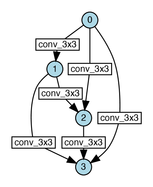
Appendix I Visualization of Search Result
Figures 5, 6(a) and 6(b) shows some architectures obtained in our experiments. The circles correspond to nodes and the number in each circle denotes the index of the node.