ADMoE: Anomaly Detection with Mixture-of-Experts from Noisy Labels

Yue Zhao¹, Guoqing Zheng², Subhabrata Mukherjee², Robert McCann³, Ahmed Awadallah²
The project is primarily done at Microsoft Research.

Abstract

Existing works on anomaly detection (AD) rely on clean labels from human annotators that are expensive to acquire in practice. In this work, we propose a method to leverage weak/noisy labels (e.g., risk scores generated by machine rules for detecting malware) that are cheaper to obtain for anomaly detection. Specifically, we propose ADMoE, the first framework for anomaly detection algorithms to learn from noisy labels. In a nutshell, ADMoE leverages Mixture-of-experts (MoE) architecture to encourage specialized and scalable learning from multiple noisy sources. It captures the similarities among noisy labels by sharing most model parameters, while encouraging specialization by building “expert” sub-networks. To further juice out the signals from noisy labels, ADMoE uses them as input features to facilitate expert learning. Extensive results on eight datasets (including a proprietary enterprise security dataset) demonstrate the effectiveness of ADMoE, where it brings up to 34% performance improvement over not using it. Also, it outperforms a total of 13 leading baselines with equivalent network parameters and FLOPS. Notably, ADMoE is model-agnostic to enable any neural network-based detection methods to handle noisy labels, where we showcase its results on both multiple-layer perceptron (MLP) and leading AD method DeepSAD.

1 Introduction

Anomaly detection (AD), also known as outlier detection, is a crucial learning task with many real-world applications, including malware detection (Nguyen et al. 2019), anti-money laundering (Lee et al. 2020), rare-disease detection (Li et al. 2018) and so on. Although there are numerous detection algorithms (Aggarwal 2013; Pang et al. 2021; Zhao, Rossi, and Akoglu 2021; Liu et al. 2022), existing AD methods assume the availability of (partial) labels that are clean (i.e. without noise), and cannot learn from weak/noisy labels¹¹1We use the terms noisy and weak interchangeably..

Simply treating noisy labels as (pseudo) clean labels leads to biased and degraded models (Song et al. 2022). Over the years, researchers have developed algorithms for classification and regression tasks to learn from noisy sources (Rodrigues and Pereira 2018; Guan et al. 2018; Wei et al. 2022), which has shown great success. However, these methods are not tailored for AD with extreme data imbalance, and existing AD methods cannot learn from (multiple) noisy sources.

Why is it important to leverage noisy labels in AD applications? Taking malware detection as an example, it is impossible to get a large number of clean labels due to the data sensitivity and the cost of annotation. However, often there exists a large number of weak/noisy historical security rules designed for detecting malware from different perspectives, e.g., unauthorized network access and suspicious file movement, which have not been used in AD yet. Though not as perfect as human annotations, they are valuable as they encode prior knowledge from past detection experiences. Also, although each noisy source may be insufficient for difficult AD tasks, learning them jointly may build competitive models as they tend to complement each other.

In this work, we propose ADMoE, (to our knowledge) the first weakly-supervised approach for enabling anomaly detection algorithms to learn from multiple sets of noisy labels. In a nutshell, ADMoE enhances existing neural-network-based AD algorithms by Mixture-of-experts (MoE) network(s) (Jacobs et al. 1991; Shazeer et al. 2017), which has a learnable gating function to activate different sub-networks (experts) based on the incoming samples and their noisy labels. In this way, the proposed ADMoE can jointly learn from multiple sets of noisy labels with the majority of parameters shared, while providing specialization and scalability via experts. Unlike existing noisy label learning approaches, ADMoE does not require explicit mapping from noisy labels to network parameters, providing better scalability and flexibility. To encourage ADMoE to develop specialization based on the noisy sources, we use noisy labels as (part of the) input features with learnable embeddings to make the gating function aware of them.

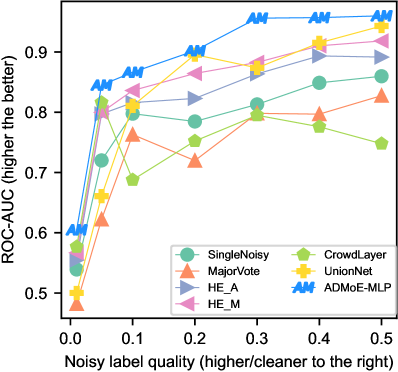
Key Results. Fig. 1 shows that a multiple layer perception (MLP) (Rosenblatt 1958) enhanced by ADMoE can largely outperform both (1(a)) leading AD algorithms as well as (1(b)) noisy-label learning methods for classification. Note ADMoE is not strictly another detection algorithm, but a general framework to empower any neural-based AD methods to leverage multiple sets of weak labels. §4 shows extensive results on more datasets, and the improvement in enhancing more complex DeepSAD (Ruff et al. 2019) with ADMoE.

In summary, the key contributions of this work include:

•

Problem formulation, baselines, and datasets. We formally define the crucial problem of using multiple sets of noisy labels for AD (MNLAD), and release the first batch of baselines and datasets for future research²²2See code and appendix: https://github.com/microsoft/admoe.
•

The first AD framework for learning from multiple noisy sources. The proposed ADMoE is a novel method with Mixture-of-experts (MoE) architecture to achieve specialized and scalable learning for MNLAD.
•

Model-agnostic design. ADMoE enhances any neural-network-based AD methods, and we show its effectiveness on MLP and state-of-the-art (SOTA) DeepSAD.
•

Effectiveness and real-world deployment. We demonstrate ADMoE’s SOTA performance on seven benchmark datasets and a proprietary enterprise security application, in comparison with two groups of leading baselines (13 in total). It brings on average 14% and up to 34% improvement over not using it, with the equivalent number of learnable parameters and FLOPs as baselines.

2 Related Work

2.1 Weakly-supervised Anomaly Detection

There exists some literature on weakly-supervised AD, and most of them fall under the “incomplete supervision” category. These semi-supervised methods assume access to a small set of clean labels and it is unclear how to extend them for multi-set noisy labels. Representative work includes XGBOD (Zhao and Hryniewicki 2018), DeepSAD (Ruff et al. 2019), DevNet (Pang, Shen, and van den Hengel 2019), PreNet (Pang et al. 2019); see Appx. B.2 for more details. We use these leading methods (that work with one set of labels) as baselines in §4.2, and demonstrate ADMoE’s performance gain in leveraging multiple sets of noisy labels.

2.2 Learning from Single Set of Noisy Labels

There have been rich literature on learning from a single set of noisy labels, including learning a label corruption/transition matrix (Patrini et al. 2017), correcting labels via meta-learning (Zheng, Awadallah, and Dumais 2021), and building robust training mechanisms like co-teaching (Han et al. 2018), co-teaching+ (Yu et al. 2019), and JoCoR (Wei et al. 2020). More details can be found in a recent survey (Han et al. 2020). These algorithms are primarily for a single set of noisy labels, and are not designed for AD tasks.

2.3 Learning from Multiple Noisy Sources

Category	SingleNoisy	LabelVote	HE_A	HE_M	CrowdLayer	UnionNet	ADMoE
Multi-source	✗	✓	✓	✓	✓	✓	✓
Single-model	✓	✓	✗	✗	✓	✓	✓
End-to-end	✓	✗	✗	✗	✓	✓	✓
Scalability	High	High	Low	Low	Med	Med	High

Table 1: Baselines and ADMoE for comparison with categorization by (first row) whether it uses multiple sets of weak labels, (second row) whether it only trains a single model, (third row) whether the training process is end-to-end and (the last row) whether it is scalable with regard to many sets of weak labels. ADMoE is an end-to-end, scalable paradigm.

MNLAD falls under weakly supervised ML (Zhou 2018), where it deals with multiple sets of inaccurate/noisy labels. Naturally, one can aggregate noisy labels to generate a “corrected” label set (Zheng, Awadallah, and Dumais 2021), while it may be challenging for AD with extreme data imbalance. Other than label correction, one may take ensembling to train multiple independent AD models for combination, e.g., one model per set of noisy labels, which however faces scalability issues while dealing with many sets of labels. What is worse, independently trained models fail to explore the interaction among noisy labels. Differently, end-to-end noisy label learning methods, including Crowd Layer (Rodrigues and Pereira 2018), DoctorNet (Guan et al. 2018), and UnionNet (Wei et al. 2022), can directly learn from multiple sets of noisy labels and map each set of noisy labels to part of the network (e.g., transition matrix), encouraging the model to learn knowledge from all noisy labels collectively. Although they yield great performance in crowd-sourcing scenarios with a small number of annotators, they do not scale in MNLAD with many sets of “cheap” noisy labels due to this explicit one-to-one mapping. Also, each set of noisy AD labels may be only good at certain anomalies as a biased annotator. Consequently, explicit one-to-one mapping (e.g., transition matrix) from a single set of labels to a network in existing classification works is not ideal for MNLAD. ADMoE lifts this constraint to allow many-to-many mapping, improving model scalability and robustness for MNLAD.

We summarize the methods for learning from multiple sources of noisy labels in Table 1 categorized as: (1) SingleNoisy trains an AD model using only one set of weak labels, which sets the lower bound of all baselines. (2) LabelVote trains an AD model based on the consensus of weak labels via majority vote. (3) HyperEnsemble (Wenzel et al. 2020) trains an individual model for each set of noisy labels (i.e., $k$ models for $k$ sets of labels), and combines their anomaly scores by averaging (i.e., HE_A) and maximizing (i.e., HE_M). (4) CrowdLayer (Rodrigues and Pereira 2018) tries to reconstruct the input weak labels during training. (5) UnionNet (Wei et al. 2022) learns a transition matrix for all weak labels together. Note that they are primarily for classification and not tailored for anomaly detection. Nonetheless, we adapt the methods in Table 1 as baselines. In §4.3, we show ADMoE outperforms all these methods.

3 AD from Multiple Sets of Noisy Labels

In §3.1, we formally present the problem of AD with multiple sets of noisy labels, followed by the discussion on why multiple noisy sources help AD in §3.2. Motivated by above, we describe the proposed ADMoE framework in §3.3.

3.1 Problem Statement

We consider the problem of anomaly detection with multiple sets of weak/noisy labels. We refer to this problem as MNLAD, an acronym for using multiple sets of noisy labels for anomaly detection. We present the problem definition here.

Problem 1 (MNLAD)

Given an anomaly detection task with input feature $\mathbf{X}\in\mathbb{R}^{n\times d}$ (e.g., $n$ samples and $d$ features) and $t$ sets of noisy/weak labels $\mathcal{Y}_{w}=\{\mathbf{y}_{w,1},\dots,\mathbf{y}_{w,t}\}$ (each in $\mathbb{R}^{n}$ ), build a detection model $M$ to leverage all information to achieve the best performance.

Existing AD methods (Aggarwal 2013; Pang et al. 2021; Han et al. 2022) can (at best) treat one set of noisy labels from $\mathcal{Y}^{w}$ as (pseudo) clean labels to train a model. None of them leverages multiple sets of noisy labels $\mathcal{Y}^{w}$ collectively.

3.2 Why and How Do Multiple Sets of Weak Labels Help in Anomaly Detection?

Benefits of joint learning in MNLAD. AD benefits from model combination and ensemble learning from diverse base models (Aggarwal and Sathe 2017; Zhao et al. 2019; Ding, Zhao, and Akoglu 2022), and the improvement is expected when base models make complementary errors (Zimek, Campello, and Sander 2014; Aggarwal and Sathe 2017). Multiple sets of noisy labels are natural sources for ensembling with built-in diversity, as they reflect distinct detection aspects and historical knowledge. Appx. A Fig. A1 shows that averaging the outputs from multiple AD models (each trained on one set of noisy labels) leads to better results than training each model independently; this observation holds true for both deep (neural) AD models (e.g., PreNet in Appx. Fig. 1(a)) and shallow models (e.g., XGBOD in Appx. Fig. 1(b)). This example justifies the benefit of learning from multiple sets of noisy labels; even simple averaging in MNLAD can already “touch” the performance upper bound (i.e., training a model using all clean labels).

3.3 ADMoE: Specialized and Scalable Anomaly Detection with Multiple Sets of Noisy Labels

Motivation. After reviewing gaps and opportunities in existing works, we argue the ideal design for MNLAD should fulfill the following requirements: (i) encourage specialization from different noisy sources but also explore their similarity (ii) scalability to handle an increasing number of noisy sources and (iii) generality to apply to various AD methods.

Overview of ADMoE. In this work, (for the first time) we adapt Mixture-of-experts (MoE) architecture/layer (Jacobs et al. 1991; Shazeer et al. 2017) (see preliminary in §3.3.1) to AD algorithm design for MNLAD. Specifically, we propose model-agnostic ADMoE ³³3Throughout the paper, we slightly abuse the term ADMoE to refer to both our overall framework and the proposed MoE layer. to enhance any neural network-based AD method via: (i) mixture-of-experts (MoE) layers to do specialized and scalable learning from noisy labels and (ii) noisy-label aware expert activation by using noisy labels as (part of the) input with learnable embedding to facilitate specialization. Refer to Fig. 2(c) for an illustration of applying ADMoE to a simple MLP, where we add an ADMoE layer between the dense layers and output layer for MNLAD, and use noisy labels directly as input with learnable embedding to help ADMoE to better specialize. Other neural-network-based AD methods can follow the same procedure to be enhanced by ADMoE (i.e., inserting ADMoE layers before the output layer and using noisy labels as input). In the following subsections, we give a short background of MoE and then present the design of ADMoE.

3.3.1 Preliminary on Mixture-of-experts (MoE) Architecture.

The original MoE (Jacobs et al. 1991) is designed as a dynamic learning paradigm to allow different parts (i.e., experts) of a network to specialize for different samples. More recent (sparsely-gated) MoE (Shazeer et al. 2017) has been shown to improve model scalability for natural language processing (NLP) tasks, where models can have billions of parameters (Du et al. 2022). The key difference between the original MoE and the sparse MoE is the latter builds more experts (sub-networks) for a large model but only activates a few of them for scalability and efficiency.

Basically, MoE splits specific layer(s) of a (large) neural network into $m$ small “experts” (i.e., sub-networks). It uses top- $k$ gating to activate $k$ experts ( $k<m$ or $k\ll m$ for sparse MoE) for each input sample computation as opposed to using the entire network as standard dense models. More specifically, MoE uses a differentiable gating function $G(\cdot)$ to calculate the activation weights of each expert. It then aggregates the weighted outputs of the top- $k$ experts with the highest activation weights as the MoE layer output. For example, the expert weights $\bm{\beta}^{j}\in\mathbb{R}^{m}$ of the $j$ -th sample is a function of input data by the gating $G(\cdot)$ , i.e., $\bm{\beta}^{j}=G(\mathbf{X}^{j})$ .

Till now, MoE has been widely used in multi-task learning (Zheng et al. 2019), video captioning (Wang et al. 2019), and multilingual neural machine translation (NMT) (Dai et al. 2022) tasks. Taking NMT as an example, prior work (Dai et al. 2022) shows that MoE can help learn a model from diverse sources (e.g., different languages), where they share the most common parameters but also specialize for individual source via “experts” (sub-networks). We combine the strengths of original and sparse MoE for our ADMoE.

3.3.2 Capitalizing Mixture-of-experts (MoE) Architecture for MNLAD.

It is easy to see the connection between MoE’s applications (e.g., multilingual machine translation) and MNLAD—in both cases MoE can help learn from diverse sources (e.g., multiple sets of noisy labels in MNLAD) to capture the similarity via parameter sharing while encouraging specialization via expert learning.

By recognizing this connection, we (for the first time), introduce MoE architecture for weakly supervised AD with noisy labels (i.e., MNLAD), called ADMoE. Similar to other works that use MoE, proposed ADMoE keeps (does not alter) an (AD) algorithm’s original layers before the output layer (e.g., dense layers in an MLP) to explore the agreement among noisy sources via shared parameters, while inserting an MoE layer before the output layer to learn from each noisy source with specialization (via the experts/sub-networks). In an ideal world, each expert is good at handling samples from different noisy sources and updated only with more accurate sets of noisy labels. As the toy example shown in Fig. 2(c) to apply ADMoE on an MLP for AD, we insert an ADMoE layer between the dense layers and the output layer: where the ADMoE layer contains four experts, and the gating activates only the top two for each input example.

For the $j$ -th sample, the MoE layer’s output $O^{j}$ is shown in Eq. (1) as a weighted sum of all activated experts’ outputs, where $E_{i}(\cdot)$ denotes the $i$ -th expert network, and $h^{j}$ is the output from the dense layer (as the input to ADMoE). $\beta_{i}^{j}$ is the weight of the $i$ -th expert assigned by the gating function $G(\cdot)$ , and we describe its calculation in Eq. (2). Although Eq. (1) enumerates all $m$ experts for aggregation, only the top- $k$ experts with non-negative weights $\beta_{i}^{j}>0$ are used.

O^{j}=\sum_{i=1}^{m}\beta_{i}^{j}E_{i}(h^{j})

(1)

Improving ADMoE with Noisy-Label Aware Expert Activation. The original MoE calculates the activation weights with only the raw input feature $\mathbf{X}$ (see §3.3.1), which can be improved in MNLAD with the presence of noisy labels. To such end, we explicitly make the gating function $G(\cdot)$ aware of noisy labels $\mathcal{Y}_{w}$ while calculating the weights for (activating) experts. Intuitively, $t$ sets of noisy labels can be expressed as $t$ -element binary vectors (0 means normalcy and 1 means abnormality). However, it is hard for neural networks to directly learn binary inputs (Buckman et al. 2018). Thus, we propose to learn a $\mathbb{R}^{t\times e}$ continuous embedding $Emb(\cdot)$ for noisy labels ( $e$ is embedding dimension), and use both the raw input features $\mathbf{X}$ in $d$ dims and the average of the embedding in $e$ dims as the input of the gating. As such, the expert weights for the $j$ -th sample $\bm{\beta}^{j}$ can be calculated with Eq. (2), and plugged back into Eq. (1) for ADMoE output.

\bm{\beta}^{j}=G\left(\mathbf{X}^{j},Emb(\mathcal{Y}_{w}^{j})\right)

(2)

Loss Function. ADMoE is strictly an enhancement framework for MNLAD other than a new detection algorithm, and thus we do not need to design a new loss function but just enrich the original loss $\mathcal{L}_{o}$ of the underlying AD algorithm (e.g., cross-entropy for a simple MLP). While calculating the loss in each batch of data, we randomly sample one set of noisy labels treated as the (pseudo) clean labels or combine the loss of all $t$ sets of noisy labels by treating them as (pseudo) clean labels. To encourage all experts to be evenly activated and not collapse on a few of them (Riquelme et al. 2021), we include an additional loss term on gating (i.e, $\mathcal{L}_{g}$ ). Putting these together, we show the loss for the $j$ -th training sample in Eq. (3), where the first term encourages equal activation of experts with $\alpha$ as the load balancing factor, and the second part is the loss of the $j$ -th sample, which depends on the MoE layer output $O^{j}$ in Eq. (1) and the corresponding noisy labels $\mathcal{Y}_{w}^{j}$ (either one set or all in loss calculation).

\mathcal{L}^{j}=\alpha\mathcal{L}_{g}+\mathcal{L}_{o}\left(O^{j},\mathcal{Y}_{w}^{j}\right)

(3)

Remark on the Number of ADMoE Layers and Sparsity. Similar to the usage in NLP, one may use multiple ADMoE layers in an AD model (e.g., every other layer), especially for the AD models with complex structures like transformers (Li, Liu, and Jiao 2022). In this work, we only show inserting the ADMoE layer before the output layer (see the illustration in Fig. 2(c)) of MLP, while future work may explore more extensive use of ADMoE layers in complex AD models. As AD models are way smaller (Pang et al. 2021), we do not enforce gating sparsity as in NLP models (Shazeer et al. 2017). See ablation studies on the total number of experts and the number of activated experts in §4.4.3.

3.3.3 Advantages and Properties of ADMoE

Implicit Mapping of Noisy Labels to Experts with Better Scalability. The proposed ADMoE (Fig. 2(c)) is more scalable than existing noisy-label learning methods for classification, e.g., CrowdLayer (Fig. 2(a)) and UnionNet (Fig. 2(b)). As discussed in §2.3, these methods explicitly map each set of noisy labels to part of the network. With more sets of noisy labels, the network parameters designated for (recovering or mapping) noisy labels increase proportionately. In contrast, ADMoE does not enforce explicit one-to-one mapping from noisy labels to experts. Thus, its many-to-many mapping becomes more scalable with many noisy sources.

Extension with Clean Labels. Our design also allows for easy integration of clean labels. In many AD tasks, a small set of clean labels are feasible, where ADMoE can easily use them. No update is needed for the network design, but simply treating the clean label as “another set of noisy labels” with higher weights. See §4.4.4 for experiment results.

4 Experiments

We design experiments to answer the following questions:

1.

How do ADMoE-enhanced methods compare to SOTA AD methods that learn from a single set of labels? (§4.2)
2.

How does ADMoE compare to leading (multiple sets of) noisy label learning methods for classification? (§4.3)
3.

How does ADMoE perform under different settings, e.g., varying num. of experts and clean label ratios? (§4.4)

4.1 Experiment Setting

Data	# Samples	# Features	# Anomaly	% Anomaly	Category
ag news	10000	768	500	5.00	NLP
aloi	49534	27	1508	3.04	Image
mnist	7603	100	700	9.21	Image
spambase	4207	57	1679	39.91	Doc
svhn	5208	512	260	5.00	Image
Imdb	10000	768	500	5.00	NLP
Yelp	10000	768	500	5.00	NLP
security^∗	5525	21	378	6.84	Security

Table 2: Data description of the eight datasets used in this study: the top seven datasets are adapted from AD repo., e.g., DAMI (Campos et al. 2016) and ADBench (Han et al. 2022), and security^∗ is a proprietary enterprise-security dataset.

Benchmark Datasets. As shown in Table 2, we evaluate ADMoE on seven public datasets adapted from AD repositories (Campos et al. 2016; Han et al. 2022) and a proprietary enterprise-security dataset (with $t=3$ sets of noisy labels). Note that these public datasets do not have existing noisy labels for AD, so we simulate $t=4$ sets of noisy labels per dataset via two methods:

1.

Label Flipping (Zheng, Awadallah, and Dumais 2021) generates noisy labels by uniformly swapping anomaly and normal classes at a designated noise rate.
2.

Inaccurate Output uses varying percentages of ground truth labels to train $t$ diverse classifiers, and considers their (inaccurate) predictions as noisy labels. With more ground truth labels to train a classifier, its prediction (e.g., noisy labels) will be more accurate—we control the noise levels by the availability of ground truth labels.

In this work, we use the noisy labels simulated by Inaccurate Output since that is more realistic and closer to real-world applications (e.g., noise is not random), while we also release the datasets by Label Flipping for broader usage. We provide a detailed dataset description in Appx. B.1.

Two Groups of Baselines are described below:

1.

Leading AD methods that can only handle a single set of labels to show ADMoE’s benefit of leveraging multiple sets of noisy labels. These include SOTA AD methods: (1) XGBOD (Zhao and Hryniewicki 2018) (2) PreNet (Pang et al. 2019) (3) DevNet (Pang, Shen, and van den Hengel 2019) (4) DeepSAD (Ruff et al. 2019), and popular classification methods: (5) MLP (6) XGBoost (Chen and Guestrin 2016) (7) LightGBM (Ke et al. 2017). We provide detailed descriptions in Appx. §B.2.
2.

Leading methods (for classification) that handle multiple sets of noisy labels (we adapt them for MNLAD; see §2.3 and Table 1 for details): (1) SingleNoisy (2) LabelVote (3) HyperEnsemble (Wenzel et al. 2020) that averages $t$ models’ scores (referred as HP_A) or takes their max (referred as HP_M) (4) CrowdLayer (Rodrigues and Pereira 2018) and latest (5) UnionNet (Wei et al. 2022).

Dataset	XGBOD	PreNet	DevNet	LGB	MLP	ADMoE- MLP	$\Delta$ Perf.	DeepSAD	ADMoE- DeepSAD	$\Delta$ Perf.
agnews	0.8277	0.903	0.8789	0.7991	0.8293	0.946	+14.07%	0.7627	0.9423	+23.55%
aloi	0.6312	0.6209	0.6057	0.6406	0.6078	0.8142	+33.96%	0.6552	0.7458	+13.83%
imdb	0.6898	0.7741	0.7372	0.6667	0.7335	0.8872	+20.95%	0.6688	0.8881	+32.79%
mnist	0.9887	0.9869	0.9777	0.9907	0.9821	0.9913	+0.94%	0.96	0.9891	+3.03%
spamspace	0.9736	0.9683	0.9645	0.9743	0.9706	0.9744	+0.39%	0.955	0.9804	+2.66%
svhn	0.8585	0.8185	0.837	0.8016	0.7847	0.9022	+14.97%	0.7705	0.9025	+17.13%
yelp	0.7778	0.8699	0.8689	0.7348	0.7955	0.9535	+19.86%	0.7781	0.9355	+20.23%
security^∗	0.7479	0.7415	0.7498	0.7335	0.7363	0.7767	+5.49%	0.7928	0.8108	+2.27%
Average	0.8119	0.8353	0.8274	0.7926	0.8049	0.9056	+13.83%	0.7929	0.8993	+14.44%

Table 3: Performance comparison between ADMoE-enhanced AD methods and leading AD methods (that can only use one set of labels) at noisy level 0.2. The best performance is highlighted in bold per dataset (row). ADMoE-based methods (ADMoE-MLP and ADMoE-DeepSAD denote ADMoE-enhanced MLP and DeepSAD) outperform all baselines. ADMoE brings on average 13.83% and up to 33.96% improvement over the original MLP, and on average 14.44% and up to 32.79% improvement over DeepSAD. Note that all the neural-network models use the equivalent numbers of parameters and training FLOPs.

Backbone AD Algorithms, Model Capacity, and Hyperparameters. We show the generality of ADMoE to enhance (i) simple MLP and (ii) SOTA DeepSAD (Ruff et al. 2019). To ensure a fair comparison, we ensure all methods have the equivalent number of trainable parameters and FLOPs. See Appx. C.2 and code for additional settings (e.g., hyperparameters) in this study. All experiments are run on an Intel i7-9700 @3.00 GH, 64GB RAM, 8-core workstation with an NVIDIA Tesla V100 GPU.

Evaluation. For methods with built-in randomness, we run four independent trials and take the average, with a fixed dataset split (70% train, 25% for test, 5% for validation). Following AD research tradition (Aggarwal and Sathe 2017; Zhao et al. 2019; Lai et al. 2021; Han et al. 2022), we report ROC-AUC as the primary metric, while also showing additional results of average precision (AP) in Appx. C.3.

4.2 Comparison Between ADMoE Methods and Leading AD Methods (Q1)

Fig. 1(a) and Fig. 3 show that ADMoE enables MLP and DeepSAD to use multiple sets of noisy labels, which outperform leading AD methods that can use only one set of labels, at varying noisy label qualities (x-axis). We further use Table 3 to compare them at noisy label quality 0.2 to understand the specific gain of ADMoE using multiple sets of noisy labels. The third block of the table shows that ADMoE brings on average 13.83%, and up to 33.96% (aloi; 3-rd row) improvements to a simple MLP. Additionally, the fourth block of the table further demonstrates that ADMoE enhances DeepSAD for using multiple noisy labels, with on average 14.44%, and up to 32.79% (imdb; 4-th row) gains. These results demonstrate the benefit of using ADMoE to enable AD algorithms to learn from multiple noisy sources.

ADMoE shows larger improvement when labels are more noisy (to the left of x-axis of Fig. 3). We observe that ADMoE-DeepSAD brings up to 60% of ROC-AUC improvement over the best-performing AD algorithm at noisy label quality 0.01 (see Fig. 3(c) for imdb). This observation is meaningful as we mostly need an approach to improve detection quality when the labels are extremely noisy, where ADMoE yields more improvement. Fig. 3 also demonstrates when the labels are less noisy (to the right of the x-axis), the performance gaps among methods are smaller since the diversity among noisy sources is also reduced—using any set of noisy labels is sufficient to train a good AD model. Also, note that ADMoE-DeepSAD shows better performance than ADMoE-MLP with more noisy labels. This results from the additional robustness of the underlying semi-supervised method DeepSAD with access to unlabeled data.

4.3 Comparison Between ADMoE and Noisy Label Learning Methods (Q2)

Dataset	Single Noisy	Major Vote	HE_A	HE_M	Crowd Layer	Union Net	ADMoE
agnews	0.7185	0.5729	0.7824	0.8101	0.8543	0.7412	0.8549
aloi	0.531	0.479	0.5195	0.5579	0.5495	0.5773	0.5842
imdb	0.5967	0.5521	0.6587	0.6599	0.6219	0.5918	0.6577
mnist	0.9482	0.9467	0.9598	0.9563	0.9644	0.6767	0.9655
spamspace	0.9626	0.9655	0.9584	0.9586	0.7654	0.9567	0.9655
svhn	0.7201	0.6222	0.7971	0.7998	0.8161	0.6608	0.8451
yelp	0.6777	0.5708	0.7298	0.7358	0.7418	0.7133	0.7533
security^∗	0.7363	0.7653	0.7526	0.7484	0.7374	0.7435	0.7767
Average	0.7363	0.6843	0.7722	0.7783	0.7563	0.7014	0.8003

Table 4: Performance comparison between ADMoE and leading noisy-label learning methods (in Table 1) on an MLP at noisy label quality 0.05. The best performance is highlighted in bold per dataset (row). ADMoE mostly outperforms baselines, with on avg. 9.4% and up to 19% improvement over SingleNoisy which trains w/ a set of noisy labels.

ADMoE also shows an edge over SOTA classification methods that learn from multiple sets of noisy labels⁴⁴4We adapt these classification methods (Table 1) for MNLAD., as shown in Fig. 1(b) and 4. We also analyze the comparison at noisy label quality 0.05 in Table 4. where ADMoE ranks the best in 7 out of 8 datasets. In addition to better detection accuracy, ADMoE only builds a single model, and is thus faster than HE_E and HE_M which requires building $t$ independent models to aggregate predictions. We credit ADMoE’s performance over SOTA algorithms including CrowdLayer and UnionNet to its implicit mapping of noisy labels to experts (§3.3.3).

4.4 Ablation Studies and Other Analysis (Q3)

4.4.1. Case Study: How does ADMoE Help?

Although MoE is effective in various NLP tasks, it is often challenging to contextualize how each expert responds to specific groups of samples due to the complexity of NLP models (Shazeer et al. 2017; Zheng et al. 2019; Zuo et al. 2021). Given that AD models are much smaller and we use only one MoE layer before the output layer, we present an interesting case study (MLP with 4 experts where top 1 gets activated) in Table 5. We find each expert achieves the highest ROC-AUC on the subsamples where it gets activated by gating (see the diagonal), and they are significantly better than training an individual model with the same architecture (see the last column). Thus, each expert does develop a specialization in the subsamples they are “responsible” for.

Activated Expert	Expert 1	Expert 2	Expert 3	Expert 4	Comp.
Subsamples for Expert 1	0.8554	0.8488	0.8458	0.8440	0.7741
Subsamples for Expert 2	0.8995	0.9043	0.8913	0.8943	0.7976
Subsamples for Expert 3	0.8633	0.8643	0.8729	0.8665	0.8049
Subsamples for Expert 4	0.7903	0.7888	0.7775	0.8066	0.7134

Table 5: Perf. breakdown of each expert and a comparison model (w/ the same capacity as each expert but trained independently; last col.) on subsamples activated for each expert by MoE on Yelp. We highlight the best model per row in bold. The specialized expert performs the best in their assigned subsamples by gating, i.e., the diagonal is all in bold.

4.4.2 Ablation on Using MoE and Noisy Labels as Inputs in ADMoE.

Additionally, we analyze the effect of using (i) ADMoE layer and (ii) noisy labels as input features in Fig. 5 and Appx. Fig. C2. First, ADMoE performs the best while using these two techniques jointly in most cases, and significantly better than not using them ( ). Second, ADMoE helps the most when labels are noisier (to the left of the x-axis) with an avg. of 2% improvement over only using noisy labels as input ( ). As expected, its impact is reduced with less noisy labels (i.e., closer to the ground truth): in that case, noisy labels are more similar to each other and specialization with ADMoE is therefore limited.

4.4.3 Effect of Number of Experts ( $m$ ) and top- $k$ Gating.

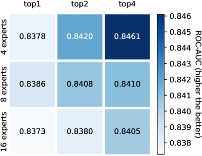
We vary the number of activated (x-axis) and total (y-axis) experts in ADMoE, and compare their detection accuracy in Fig. 6 and Appx. Fig. C3. The results suggest that the best choice is data-dependent, and we use $m=4$ and $k=2$ for all the datasets in the experiments.

4.4.4 Performance on Varying Number of Clean Labels.

As introduced in §3.3.3, one merit of ADMoE is the easy integration of clean labels when available. Fig. 7 and Appx. Fig. C4 show that ADMoE can leverage the available clean labels to achieve higher performance. Specifically, ADMoE with only 8% clean labels can achieve similar or better results than that of using all available clean labels on spamspace and svhn.

5 Conclusions

We propose ADMoE, a model-agnostic learning framework, to enable anomaly detection algorithms to learn from multiple sets of noisy labels. Leveraging Mixture-of-experts (MoE) architecture from the NLP domain, ADMoE is scalable in building specialization based on the diversity among noisy sources. Extensive experiments show that ADMoE outperforms a wide range of leading baselines, bringing on average 14% improvement over not using it. Future work can explore its usage with complex detection algorithms.

References

Aggarwal (2013) Aggarwal, C. C. 2013. Outlier Analysis. Springer. ISBN 978-1-4614-6395-5.
Aggarwal and Sathe (2017) Aggarwal, C. C.; and Sathe, S. 2017. Outlier ensembles: An introduction. Springer.
Breiman (2001) Breiman, L. 2001. Random forests. Machine learning, 45(1): 5–32.
Breiman et al. (2017) Breiman, L.; Friedman, J. H.; Olshen, R. A.; and Stone, C. J. 2017. Classification and regression trees. Routledge.
Buckman et al. (2018) Buckman, J.; Roy, A.; Raffel, C.; and Goodfellow, I. 2018. Thermometer encoding: One hot way to resist adversarial examples. In International Conference on Learning Representations.
Campos et al. (2016) Campos, G. O.; Zimek, A.; Sander, J. Ã. ¶. r.; Campello, R. J.; Micenkov Ã ¡, B.; Schubert, E.; Assent, I.; and Houle, M. E. 2016. On the evaluation of unsupervised outlier detection: measures, datasets, and an empirical study, volume 30. Springer US.
Chen and Guestrin (2016) Chen, T.; and Guestrin, C. 2016. Xgboost: A scalable tree boosting system. In Proceedings of the 22nd acm sigkdd international conference on knowledge discovery and data mining, 785–794. ACM.
Dai et al. (2022) Dai, D.; Dong, L.; Ma, S.; Zheng, B.; Sui, Z.; Chang, B.; and Wei, F. 2022. StableMoE: Stable Routing Strategy for Mixture of Experts. In Proceedings of ACL, 7085–7095.
Ding, Zhao, and Akoglu (2022) Ding, X.; Zhao, L.; and Akoglu, L. 2022. Hyperparameter Sensitivity in Deep Outlier Detection: Analysis and a Scalable Hyper-Ensemble Solution. ArXiv preprint, abs/2206.07647.
Du et al. (2022) Du, N.; Huang, Y.; Dai, A. M.; Tong, S.; Lepikhin, D.; Xu, Y.; Krikun, M.; Zhou, Y.; Yu, A. W.; Firat, O.; et al. 2022. Glam: Efficient scaling of language models with mixture-of-experts. In International Conference on Machine Learning, 5547–5569. PMLR.
Guan et al. (2018) Guan, M.; Gulshan, V.; Dai, A.; and Hinton, G. 2018. Who said what: Modeling individual labelers improves classification. In Proceedings of the AAAI conference on artificial intelligence, volume 32.
Han et al. (2020) Han, B.; Yao, Q.; Liu, T.; Niu, G.; Tsang, I. W.; Kwok, J. T.; and Sugiyama, M. 2020. A survey of label-noise representation learning: Past, present and future. ArXiv preprint, abs/2011.04406.
Han et al. (2018) Han, B.; Yao, Q.; Yu, X.; Niu, G.; Xu, M.; Hu, W.; Tsang, I.; and Sugiyama, M. 2018. Co-teaching: Robust training of deep neural networks with extremely noisy labels. Advances in neural information processing systems, 31.
Han et al. (2022) Han, S.; Hu, X.; Huang, H.; Jiang, M.; and Zhao, Y. 2022. Adbench: Anomaly detection benchmark. In Advances in Neural Information Processing Systems (NeurIPS).
Jacobs et al. (1991) Jacobs, R. A.; Jordan, M. I.; Nowlan, S. J.; and Hinton, G. E. 1991. Adaptive mixtures of local experts. Neural computation, 3: 79–87.
Ke et al. (2017) Ke, G.; Meng, Q.; Finley, T.; Wang, T.; Chen, W.; Ma, W.; Ye, Q.; and Liu, T.-Y. 2017. Lightgbm: A highly efficient gradient boosting decision tree. Advances in neural information processing systems, 30.
Lai et al. (2021) Lai, K.-H.; Zha, D.; Wang, G.; Xu, J.; Zhao, Y.; Kumar, D.; Chen, Y.; Zumkhawaka, P.; Wan, M.; Martinez, D.; et al. 2021. Tods: An automated time series outlier detection system. In Proceedings of the aaai conference on artificial intelligence, volume 35, 16060–16062.
Lee et al. (2020) Lee, M.-C.; Zhao, Y.; Wang, A.; Liang, P. J.; Akoglu, L.; Tseng, V. S.; and Faloutsos, C. 2020. Autoaudit: Mining accounting and time-evolving graphs. In 2020 IEEE International Conference on Big Data (Big Data), 950–956. IEEE.
Li, Liu, and Jiao (2022) Li, S.; Liu, F.; and Jiao, L. 2022. Self-training multi-sequence learning with Transformer for weakly supervised video anomaly detection. Proceedings of the AAAI, Virtual, 24.
Li et al. (2018) Li, W.; Wang, Y.; Cai, Y.; Arnold, C.; Zhao, E.; and Yuan, Y. 2018. Semi-supervised Rare Disease Detection Using Generative Adversarial Network. In NeurIPS Workshop on Machine Learning for Health (ML4H).
Liu et al. (2022) Liu, K.; Dou, Y.; Zhao, Y.; Ding, X.; Hu, X.; Zhang, R.; Ding, K.; Chen, C.; Peng, H.; Shu, K.; Sun, L.; Li, J.; Chen, G. H.; Jia, Z.; and Yu, P. S. 2022. BOND: Benchmarking Unsupervised Outlier Node Detection on Static Attributed Graphs. In Thirty-sixth Conference on Neural Information Processing Systems Datasets and Benchmarks Track.
Nguyen et al. (2019) Nguyen, T. D.; Marchal, S.; Miettinen, M.; Fereidooni, H.; Asokan, N.; and Sadeghi, A.-R. 2019. DÏoT: A federated self-learning anomaly detection system for IoT. In 2019 IEEE 39th International conference on distributed computing systems (ICDCS), 756–767. IEEE.
Pang et al. (2021) Pang, G.; Shen, C.; Cao, L.; and Hengel, A. V. D. 2021. Deep learning for anomaly detection: A review. ACM Computing Surveys (CSUR), 54(2): 1–38.
Pang et al. (2019) Pang, G.; Shen, C.; Jin, H.; and Hengel, A. v. d. 2019. Deep weakly-supervised anomaly detection. ArXiv preprint, abs/1910.13601.
Pang, Shen, and van den Hengel (2019) Pang, G.; Shen, C.; and van den Hengel, A. 2019. Deep anomaly detection with deviation networks. In Proceedings of the 25th ACM SIGKDD international conference on knowledge discovery & data mining, 353–362.
Patrini et al. (2017) Patrini, G.; Rozza, A.; Krishna Menon, A.; Nock, R.; and Qu, L. 2017. Making deep neural networks robust to label noise: A loss correction approach. In Proceedings of the IEEE conference on computer vision and pattern recognition, 1944–1952.
Riquelme et al. (2021) Riquelme, C.; Puigcerver, J.; Mustafa, B.; Neumann, M.; Jenatton, R.; Susano Pinto, A.; Keysers, D.; and Houlsby, N. 2021. Scaling vision with sparse mixture of experts. Advances in Neural Information Processing Systems, 34: 8583–8595.
Rodrigues and Pereira (2018) Rodrigues, F.; and Pereira, F. 2018. Deep learning from crowds. In Proceedings of the AAAI conference on artificial intelligence, volume 32.
Rosenblatt (1958) Rosenblatt, F. 1958. The perceptron: a probabilistic model for information storage and organization in the brain. Psychological review, 65(6): 386.
Ruff et al. (2021) Ruff, L.; Kauffmann, J. R.; Vandermeulen, R. A.; Montavon, G.; Samek, W.; Kloft, M.; Dietterich, T. G.; and Müller, K.-R. 2021. A unifying review of deep and shallow anomaly detection. Proceedings of the IEEE.
Ruff et al. (2019) Ruff, L.; Vandermeulen, R. A.; Görnitz, N.; Binder, A.; Müller, E.; Müller, K.-R.; and Kloft, M. 2019. Deep Semi-Supervised Anomaly Detection. In International Conference on Learning Representations.
Ruff et al. (2018) Ruff, L.; Vandermeulen, R. A.; Görnitz, N.; Deecke, L.; Siddiqui, S. A.; Binder, A.; Müller, E.; and Kloft, M. 2018. Deep One-Class Classification. In Proceedings of the 35th International Conference on Machine Learning, volume 80, 4393–4402.
Shazeer et al. (2017) Shazeer, N.; Mirhoseini, A.; Maziarz, K.; Davis, A.; Le, Q.; Hinton, G.; and Dean, J. 2017. Outrageously Large Neural Networks: The Sparsely-Gated Mixture-of-Experts Layer. ICLR.
Song et al. (2022) Song, H.; Kim, M.; Park, D.; Shin, Y.; and Lee, J.-G. 2022. Learning from noisy labels with deep neural networks: A survey. IEEE Transactions on Neural Networks and Learning Systems.
Wang et al. (2019) Wang, X.; Wu, J.; Zhang, D.; Su, Y.; and Wang, W. Y. 2019. Learning to compose topic-aware mixture of experts for zero-shot video captioning. In Proceedings of the AAAI Conference on Artificial Intelligence, volume 33, 8965–8972.
Wei et al. (2020) Wei, H.; Feng, L.; Chen, X.; and An, B. 2020. Combating noisy labels by agreement: A joint training method with co-regularization. In Proceedings of the IEEE/CVF Conference on Computer Vision and Pattern Recognition, 13726–13735.
Wei et al. (2022) Wei, H.; Xie, R.; Feng, L.; Han, B.; and An, B. 2022. Deep Learning From Multiple Noisy Annotators as A Union. IEEE Transactions on Neural Networks and Learning Systems.
Wenzel et al. (2020) Wenzel, F.; Snoek, J.; Tran, D.; and Jenatton, R. 2020. Hyperparameter ensembles for robustness and uncertainty quantification. Advances in Neural Information Processing Systems, 33: 6514–6527.
Yu et al. (2019) Yu, X.; Han, B.; Yao, J.; Niu, G.; Tsang, I.; and Sugiyama, M. 2019. How does disagreement help generalization against label corruption? In International Conference on Machine Learning, 7164–7173. PMLR.
Zhao, Chen, and Jia (2023) Zhao, Y.; Chen, G. H.; and Jia, Z. 2023. TOD: GPU-accelerated Outlier Detection via Tensor Operations. Proceedings of the VLDB Endowment, 16(3).
Zhao and Hryniewicki (2018) Zhao, Y.; and Hryniewicki, M. K. 2018. XGBOD: Improving Supervised Outlier Detection with Unsupervised Representation Learning. In International Joint Conference on Neural Networks (IJCNN). IEEE.
Zhao et al. (2019) Zhao, Y.; Nasrullah, Z.; Hryniewicki, M. K.; and Li, Z. 2019. LSCP: Locally Selective Combination in Parallel Outlier Ensembles. In Proceedings of the 2019 SIAM International Conference on Data Mining, SDM 2019, 585–593. Calgary, Canada: SIAM.
Zhao, Nasrullah, and Li (2019) Zhao, Y.; Nasrullah, Z.; and Li, Z. 2019. PyOD: A Python Toolbox for Scalable Outlier Detection. Journal of Machine Learning Research (JMLR), 20(96): 1–7.
Zhao, Rossi, and Akoglu (2021) Zhao, Y.; Rossi, R.; and Akoglu, L. 2021. Automatic unsupervised outlier model selection. Advances in Neural Information Processing Systems, 34: 4489–4502.
Zheng, Awadallah, and Dumais (2021) Zheng, G.; Awadallah, A. H.; and Dumais, S. 2021. Meta label correction for noisy label learning. In Proceedings of the AAAI Conference on Artificial Intelligence, volume 35, 11053–11061.
Zheng et al. (2019) Zheng, Z.; Yuan, C.; Zhu, X.; Lin, Z.; Cheng, Y.; Shi, C.; and Ye, J. 2019. Self-supervised mixture-of-experts by uncertainty estimation. In Proceedings of the AAAI Conference on Artificial Intelligence, volume 33, 5933–5940.
Zhou (2018) Zhou, Z.-H. 2018. A brief introduction to weakly supervised learning. National science review, 5(1): 44–53.
Zimek, Campello, and Sander (2014) Zimek, A.; Campello, R. J.; and Sander, J. 2014. Ensembles for unsupervised outlier detection: challenges and research questions a position paper. Acm Sigkdd Explorations Newsletter, 15: 11–22.
Zuo et al. (2021) Zuo, S.; Liu, X.; Jiao, J.; Kim, Y. J.; Hassan, H.; Zhang, R.; Gao, J.; and Zhao, T. 2021. Taming Sparsely Activated Transformer with Stochastic Experts. In International Conference on Learning Representations.

Supplementary Material of ADMoE

Details on algorithm design, experiment setting, and additional results.

Appendix A Additional Results on Why Does AD Benefit from Multiple Sets of Noisy Labels

Appendix B Additional Experiment Setting and Results

B.1 Dataset Description

As discussed in §4.1, we use the results based on the Classification noise since that is more realistic and closer to real-world applications (e.g., noise is not at random), while we also release the datasets by Label flipping for broader usages. See our repo to access both versions of datasets.

Process of Inaccurate Output. We use varying percentages of ground truth labels to train $t$ diverse classifiers (called noisy label generators), and consider their (inaccurate) predictions as noisy labels. Naturally, with more available ground truth labels to train a classifier, its prediction (e.g., noisy labels) will be more accurate—we therefore control the noise levels by the availability of ground truth labels.

Following this approach, we generate the noisy labels for the benchmark datasets at varying percentages of ground truth labels (namely, $\{0.01,0.05,0.1,0.2,0.3,0.4,0.5\}$ ) to train classifiers (a simple feed-forward MLP (Rosenblatt 1958), decision tree (Breiman et al. 2017), and ensemble methods Random Forest (Breiman 2001) and LightGBM (Ke et al. 2017)). Please see our code for more details.

Table B1 summarizes avg. ROC-AUC of the generated noisy labels while using varying percentages of ground truth labels to train noisy label generators. Of course, with more ground truth labels, the generated noisy labels are also more accurate. Note that security^∗ comes with actual noisy labels, and thus ROC-AUC does not vary.

Clean Perc.	agnews	aloi	imdb	mnist	spam space	svhn	yelp	security^∗
0.01	0.5384	0.5154	0.5085	0.7260	0.7862	0.5164	0.5192	0.6862
0.05	0.5663	0.5330	0.5304	0.7887	0.8929	0.5773	0.5455	0.6862
0.1	0.6210	0.5540	0.5628	0.8592	0.9047	0.6132	0.5754	0.6862
0.2	0.6641	0.5957	0.6025	0.9044	0.9182	0.6496	0.6271	0.6862
0.3	0.7065	0.6303	0.6356	0.9301	0.9301	0.6827	0.6621	0.6862
0.4	0.7462	0.6503	0.6758	0.9308	0.9401	0.7224	0.7077	0.6862
0.5	0.7662	0.6701	0.7118	0.9427	0.9482	0.7531	0.7212	0.6862

Table B1: Avg. ROC-AUC of noisy labels at different noisy label qualities (higher the better). Note that security^∗’s noisy labels are not simulated and thus do not vary.

B.2 AD Algorithms and Binary Classifiers

We provide a brief description of AD algorithms below (see more details to recent literature (Ruff et al. 2021; Han et al. 2022)). Since it lacks specialized fully supervised AD methods, we discuss some SOTA binary classifiers below.

1.

Extreme Gradient Boosting Outlier Detection (XGBOD) (Zhao and Hryniewicki 2018). XGBOD uses unsupervised outlier detectors to extract representations for the underlying dataset and concatenates the newly generated features to the original feature feature for augmentation. An XGBoost classifier is then applied to the augmented feature space.
2.

Deviation Networks (DevNet) (Pang, Shen, and van den Hengel 2019) uses a prior probability to enforce a statistical deviation score of input instances.
3.

Pairwise Relation prediction-based ordinal regression Network (PReNet) (Pang et al. 2019) is a neural network-based model that defines a two-stream ordinal regression to learn the relation of instance pairs.
4.

Deep Semi-supervised Anomaly Detection (DeepSAD) (Ruff et al. 2019). DeepSAD is considered as the SOTA semi-supervised AD method. It improves the early version of unsupervised DeepSVDD (Ruff et al. 2018) by including the supervision to penalize the inverse of the distances of anomaly representation. In this way, anomalies are forced to be in the space which is away from the hypersphere center.
5.

Multi-layer Perceptron (MLP) (Rosenblatt 1958). MLP is a simple feedforward version of the neural network, which uses the binary cross entropy loss to update network parameters.
6.

Highly Efficient Gradient Boosting Decision Tree (LightGBM) (Ke et al. 2017) is a gradient boosting framework that uses tree-based learning algorithms with faster training speed, higher efficiency, lower memory usage, and better accuracy.

Appendix C More Experiment Settings and Details

C.1 Code and Reproducibility

See our datasets and code at GitHub repository https://github.com/microsoft/admoe. Part of the code is based on PyOD (Zhao, Nasrullah, and Li 2019), ADBench (Han et al. 2022), and TOD (Zhao, Chen, and Jia 2023).

C.2 Hyperparameter Setting of ADMoE and Baselines

For all baselines used in this study, we use the same set of key hyperparameters for a fair comparison. We also use algorithms default hyperparameter (HP) settings in the original paper for unique hyperparameters. More specifically, we use the same: (i) learning rate= $0.001$ ; (ii) batch size $=256$ ; and (iii) model size (number of trainable parameters $\approx 18,000$ ). We use the small validation set (5%) to choose the epoch with the highest validation performance. See our code at https://tinyurl.com/admoe22 for more details.

C.3 Results by Average Precision (AP)

Dataset	XGBOD	PreNet	DevNet	LGB	MLP	ADMoE- MLP	$\Delta$ Perf.	DeepSAD	ADMoE- DeepSAD	$\Delta$ Perf.
agnews	0.2588	0.4053	0.3851	0.2517	0.2956	0.4775	+61.54%	0.4212	0.5512	30.86%
aloi	0.0675	0.0599	0.0616	0.0564	0.0639	0.1713	+168.08%	0.1126	0.1226	8.88%
imdb	0.1043	0.1592	0.1097	0.0912	0.1211	0.1699	+40.30%	0.2312	0.3062	32.44%
mnist	0.9131	0.8939	0.8721	0.9105	0.8696	0.9284	+6.76%	0.9014	0.9472	5.08%
spamspace	0.9543	0.9261	0.9327	0.954	0.946	0.959	+1.37%	0.9327	0.9633	3.28%
svhn	0.3468	0.346	0.2928	0.3457	0.2919	0.5021	+72.01%	0.3442	0.5545	61.10%
yelp	0.1827	0.2862	0.1912	0.1519	0.1889	0.3613	+91.27%	0.295	0.4882	65.49%
avg	0.4039	0.4395	0.4065	0.3945	0.3967	0.5099	+63.05%	0.4626	0.5619	+29.59%

Table C2: Average precision (AP) comparison between ADMoE-enhanced AD methods and leading AD methods (that can only use one set of labels) at noisy level 0.2. The best performance is highlighted in bold per dataset (row). ADMoE-based methods (ADMoE-MLP and ADMoE-DeepSAD denote ADMoE-enhanced MLP and DeepSAD) outperform all baselines. ADMoE brings on average 63.05% improvement over the original MLP, and on average 29.59% improvement over DeepSAD. Note that all the neural-network models use the equivalent numbers of parameters and FLOPS.

C.4 More Ablation Results on the Use of MoE and Weak Inputs

In addition to the ablation studies in §4.4.2, we provide additional results in Fig. C2 for the effects of using ADMoE and noisy labels as inputs. Similar statements can be made. First, ADMoE performs the best while using these two techniques jointly in most cases, and significantly better than not using them ( ). Second, ADMoE helps the most when labels are noisier (to the left of the x-axis) with an avg. of 2% improvement over only using noisy labels as input ( ). As expected, its impact is reduced with less noisy labels (i.e., closer to the ground truth): in that case, noisy labels are more similar to each other and specialization with ADMoE is less useful.